代码复习用于前列腺癌诊断和Gleason分级的人工智能
发表于nature杂志的论文https://www.nature.com/articles/s41591-021-01620-2
摘要
人工智能(AI)在活检中诊断前列腺癌方面展现出潜力。然而,结果仅限于个别研究,缺乏跨国验证。竞赛已被证明是医学影像创新的加速器,但其影响力因缺乏可重复性和独立验证而受限。基于此,我们组织了PANDA挑战赛——迄今为止规模最大的组织病理学竞赛,吸引了1290名开发者参与——旨在催化开发利用10,616份数字化前列腺活检样本进行Gleason分级的可重复AI算法。我们验证了一组多样化的算法在独立跨大陆队列中达到病理学家水平,且算法开发者完全不知情。在美国和欧洲的外部验证集中,这些算法与专家泌尿病理学家达成了0.862(平方加权κ,95%置信区间,0.840–0.884)和0.868(95% CI,0.835–0.900)的一致。通过多种算法方法,成功在不同患者群体、实验室和参考标准中实现泛化,因此有必要在前瞻性临床试验中评估基于AI的Gleason评分。
数据集描述
你们在本次竞赛中的挑战是通过显微镜扫描前列腺活检样本来分类前列腺癌的严重程度。相较于大多数比赛,这个问题有两个不同寻常的特点:
-
每张单独的图像都相当大。我们很期待看到你能提出哪些策略,高效定位关注点并放大关注。
-
标签并不完美。这是一个具有挑战性的病理学领域,即使是拥有多年经验的领域专家,也不总是对如何解读幻灯片达成一致。这会使训练模型更困难,但增强了强模型提供一致评分的潜在医学价值。所有私有测试集图像和大多数公开测试集图像均由多位病理学家评分,但训练集无法实现。你可以在这里找到病理学家标签匹配的更多细节。
Files
[train/test].csv
-
image_id: ID code for the image. -
data_provider: The name of the institution that provided the data. Both the Karolinska Institute and Radboud University Medical Center contributed data. They used different scanners with slightly different maximum microscope resolutions and worked with different pathologists for labeling their images. -
isup_grade: Train only. The target variable. The severity of the cancer on a 0-5 scale. -
gleason_score: Train only. An alternate cancer severity rating system with more levels than the ISUP scale. For details on how the gleason and ISUP systems compare, see the Additional Resources tab.
[train/test]_images: The images. Each is a large multi-level tiff file. You can expect roughly 1,000 images in the hidden test set. Note that slightly different procedures were in place for the images used in the test set than the training set. Some of the training set images have stray pen marks on them, but the test set slides are free of pen marks.
train_label_masks: Segmentation masks showing which parts of the image led to the ISUP grade. Not all training images have label masks, and there may be false positives or false negatives in the label masks for a variety of reasons. These masks are provided to assist with the development of strategies for selecting the most useful subsamples of the images. The mask values depend on the data provider:
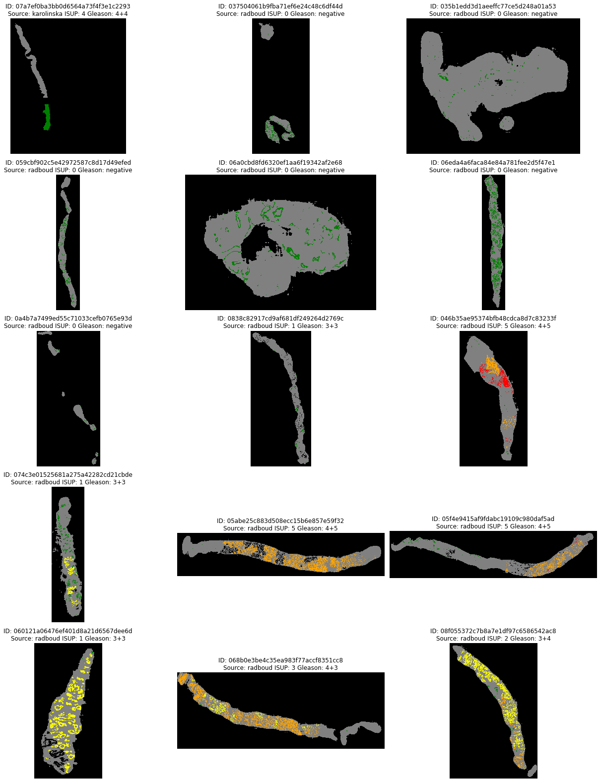
Radboud: Prostate glands are individually labelled. Valid values are:0: background (non tissue) or unknown1: stroma (connective tissue, non-epithelium tissue)2: healthy (benign) epithelium3: cancerous epithelium (Gleason 3)4: cancerous epithelium (Gleason 4)5: cancerous epithelium (Gleason 5)
Karolinska: Regions are labelled. Valid values are:0: background (non tissue) or unknown1: benign tissue (stroma and epithelium combined)2: cancerous tissue (stroma and epithelium combined)
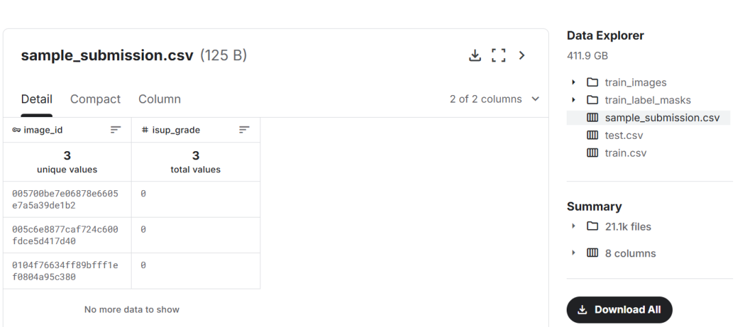
数据集下载链接:https://www.kaggle.com/competitions/prostate-cancer-grade-assessment/data
项目描述:
前列腺癌(PCa)每年新增超过100万例新诊断,是全球男性中第二常见的癌症,每年导致超过35万人死亡。降低死亡率的关键在于开发更精准的诊断方法。PCa的诊断基于前列腺组织活检的分级。这些组织样本由病理学家检查,并根据格里森分级系统进行评分。在本挑战中,你将开发通过前列腺组织样本图像检测PCa的模型,并利用目前最全面的Gleason分级多中心数据集,估计该疾病的严重程度。
分级过程包括根据肿瘤的结构生长模式,将癌组织发现并分类为所谓的格里森模式(3、4或5)。活检获得Gleason评分后,会转换为1至5分制的ISUP评分。Gleason分级系统是PCa最重要的预后标志物,而ISUP分级在决定患者治疗方式时起着关键作用。这既存在漏诊癌症的风险,也存在高分化导致不必要的治疗风险。然而,该系统在病理学家之间存在显著的观察者间差异,限制了其对个别患者的实用性。这种评级的波动可能导致不必要的治疗,甚至更糟,遗漏严重诊断。
自动化深度学习系统在准确评级PCA方面展现出一定潜力。近期研究,包括由主办方独立进行的两项研究,显示这些系统能够达到病理学家级别的性能。然而,这些系统/结果并未在多中心数据集中进行大规模测试。
你们在这里的工作将利用迄今为止最全面的Gleason分级多中心数据集,进一步完善这些努力。训练集包含约11,000张数字化H&E染色活检的全片幻灯片图像,来自两个中心。这是目前公开的最大全片图像数据集,约为CAMELYON17挑战的8倍,也是该领域最大的数字病理数据集之一,也是该领域最知名的挑战。此外,与以往的挑战不同,我们正在提供完整的诊断活检图像。我们将利用由专业泌尿病理学家评分的大型多中心测试集,评估挑战提交的适用性,以提升这一关键诊断功能。
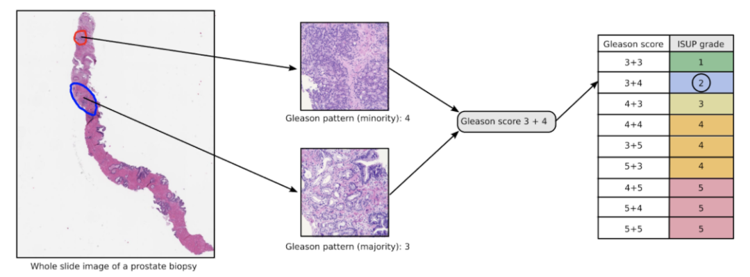
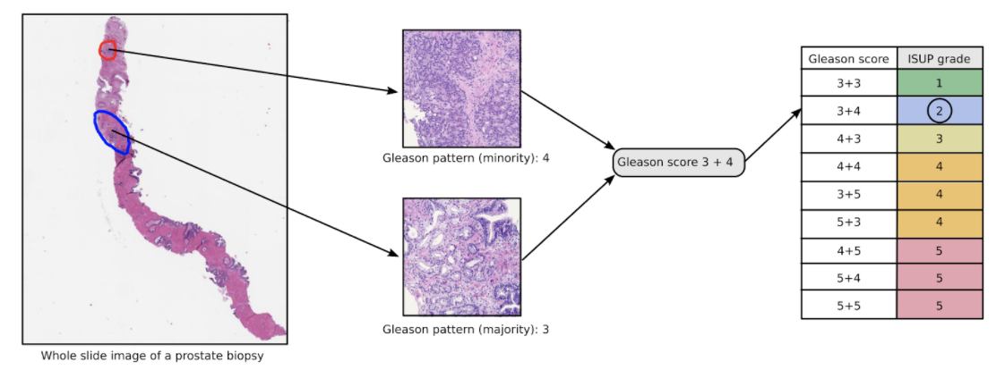
图1:Gleason分级过程示意,示例含前列腺癌活检。活检中最常见的(蓝色轮廓,Gleason模式3)和第二常见(红色轮廓,Gleason模式4)的癌症生长模式决定了Gleason评分(本次活检为3+4),随后根据国际泌尿病理学会的指导方针转换为ISUP等级(本次活检为2)。未含癌的活检在该挑战中以ISUP评分为0。
代码实现如下:
数字病理
病理学作为一门医学学科的许多基本方面几十年来基本保持不变,但该领域目前正经历向数字化学科的转型。在数字病理学中,含有组织样本的显微镜载玻片被扫描成整张载玻片图像(WSI)。这些高分辨率图像随后通过计算方式分析,而非传统在显微镜下目视评估载玻片的方法。数字病理学还带来了将计算方法应用于所得数据的可能性,尤其是基于人工智能(AI)和机器学习的图像分析技术。有关数字病理和计算病理的更多信息,参见例如(Bera, 2019)或(Niazi, 2019)。
格里森图案
本次挑战中的每个 WSI 包含从单一活检样本切出的一块,或在某些情况下是两块薄组织切片。扫描前,组织会用苏木精和伊红(H&E)染色。这是一种标准的染色方式,用于对原本透明的组织进行染色,以产生一定的对比效果。样本由腺体组织和结缔组织组成。腺体是空心结构,在WSI中可以看到白色“孔”或分支空腔。腺体的外观构成了格里森分级系统的基础。健康前列腺组织特有的腺体结构随着等级逐渐增加而逐渐丧失。评分系统识别三类:3、4和5。以下详细描述了这些模式,并在图2中举例说明:
A. 良性前列腺上皮折叠。细胞质颜色较浅,细胞核小而规则。腺体聚集在一起。B. 前列腺腺癌——Gleason型3无腺体分化丧失。小腺体浸润于良性腺体之间。细胞质通常为深色,细胞核膨大,染色质较暗,核粒显著。每个上皮单元是独立的,并且有一个腔。C. 前列腺腺癌——Gleason Pattern 4 部分失去腺体分化。尝试形成光腺体,但肿瘤未能形成完整且发育良好的腺体。这张微型照片显示了不规则的筛状癌细胞,即具有多个光的上皮片。还有一些发育不良的小腺体和融合腺体。这些都包含在格里森的第四条中。D. 前列腺腺癌——格利森型5几乎完全失去腺体分化。在基质中可见分散的单一癌细胞。格利森图样5也可能含有实心的癌细胞片或链状结构。所有显微照片在20倍镜头放大下均显示了赤木精和伊红染色。
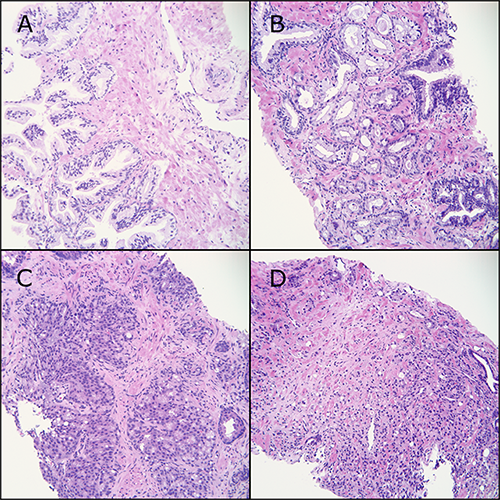
图2:用于分级的图案示例。(A)健康的腺体。(B)-(D)分别为格里森模式3至5。
ISUP等级
如图1所示(见描述标签),单次活检中的模式被用来形成Gleason评分,例如4 + 3 = 7。简单来说,如果存在多种不同的格里森模式,评分由病理学家判断为活检中最常见的模式和第二常见模式组成。少数模式必须占总面积的至少5%,例如如果模式3小于5%,则格里森得分4 + 3将变为4 + 4。此外,最高分应始终包含在成绩中。例如,活检中含有60%格里森4、37%格里森3和3%格里森5的分数应为4 + 5 = 9。详情请参见(Epstein,2016)。
根据国际泌尿病理学会(ISUP)现行指南,Gleason评分根据以下规则按1到5的等级汇总为ISUP等级:
格里森得分6 = ISUP一级 格里森得分7(3 + 4)= ISUP二级 格里森得分7(4 + 3)= ISUP三级 格里森得分8 = ISUP四级 格里森评分9-10 = ISUP五级。
如果样本中没有癌症,我们在本比赛中使用ISUP等级0的标签。
你在挑战中的任务是为每次活检提供正确的ISUP评分,准确性与病理学家判定的等级进行比较。需要注意的是,不同病理学家对同一活检的ISUP评分差异较大,这也导致本挑战中数据标签存在噪声。因此,我们邀请了多位国际病理专家分别为检测数据做标签,并由此得出共识标签。例如,参见(Egevad,2013)关于病理学家间格里森评分差异的更多信息。
计算格里森评分。
关于基于人工智能自动进行格里森活检分级的最新报告,参见例如(Ström & Kartasalo, 2020)和(Bulten, 2020)或相应的免费预印本版本,https://arxiv.org/abs/1907.01368 和 https://arxiv.org/abs/1907.07980。
Q1)什么是前列腺癌?
前列腺癌是发生在前列腺的癌症。前列腺是男性体内一个核桃大小的小腺体,它产生精液,用于滋养和运输精子。
前列腺癌是男性中最常见的癌症类型之一。通常前列腺癌生长缓慢,并最初局限于前列腺内,可能不会造成严重危害。然而,虽然某些类型的前列腺癌生长缓慢,可能只需要最低限度甚至不需要治疗,但其他类型的前列腺癌具有侵袭性,并且可以迅速扩散。
Q2)它是如何测试和检测的?
前列腺筛查测试可能包括:
-
直肠指检(DRE):在DRE期间,医生会戴上手套并润滑手指,将其插入您的直肠以检查与直肠相邻的前列腺。如果医生发现腺体的质地、形状或大小有任何异常,您可能需要进一步检查。
-
前列腺特异性抗原(PSA)检测:从您手臂的静脉中抽取血液样本,并分析其中的PSA。PSA是您的前列腺自然产生的一种物质。血液中存在少量PSA是正常的。但是,如果发现PSA水平高于正常值,则可能提示前列腺感染、炎症、增生或癌症。
如果DRE或PSA检测发现异常,医生可能会建议进行进一步检查以确定您是否患有前列腺癌,例如:
-
超声检查:如果其他检查引起担忧,医生可能会使用经直肠超声进一步评估您的前列腺。将一个雪茄大小和形状的小型探头插入您的直肠。该探头使用声波生成您前列腺的图像。
-
收集前列腺组织样本:如果初步检查结果提示前列腺癌,医生可能会建议进行一项操作以从前列腺收集细胞样本(前列腺活检)。前列腺活检通常使用一根细针插入前列腺以收集组织。组织样本在实验室中进行分析,以确定是否存在癌细胞。
Q3)格里森(Gleason)评分在整个过程中起什么作用?
当活检确认存在癌症时,下一步是确定癌细胞的侵袭性程度(级别)。实验室病理学家会检查您的癌症样本,以确定癌细胞与健康细胞的差异程度。更高的级别意味着更具侵袭性的癌症,更有可能迅速扩散。
评估前列腺癌细胞级别最常用的量表称为格里森评分。格里森评分组合两个数字,范围可以从2(非侵袭性癌症)到10(非常侵袭性癌症),不过该量表的较低部分并不常用。
Q4)我明白了,那么现在ISUP分级又是什么?
根据国际泌尿病理学学会(ISUP)的现行指南,格里森评分按照以下规则被汇总为1至5级的ISUP分级:
-
格里森评分6 = ISUP 1级
-
格里森评分7(3+4)= ISUP 2级
-
格里森评分7(4+3)= ISUP 3级
-
格里森评分8 = ISUP 4级
-
格里森评分9-10 = ISUP 5级
如果样本中没有癌症,本次比赛中我们使用标签 ISUP 0级。
Q5)数据集中的格里森评分是如何生成的?
本次挑战中的每个全切片图像(WSI)包含一条(或在某些情况下两条)从单个活检样本切取的薄组织切片。在扫描之前,组织用苏木精和伊红(H&E)染色。这是对原本透明的组织进行染色的标准方法,以产生一定的对比度。样本由腺体组织和结缔组织构成。腺体是空腔结构,在WSI中可以看到为白色的“孔洞”或分支状空腔。腺体的外观构成了格里森分级系统的基础。健康前列腺组织特征的腺体结构随着级别的升高而逐渐丧失。该分级系统识别三个类别:3、4和5。
-
[A] 良性前列腺腺体,具有折叠的上皮:细胞质苍白,细胞核小且规则。腺体聚集在一起。
-
[B] 前列腺腺癌,格里森3型模式:无腺体分化丧失。小腺体浸润在良性腺体之间。细胞质通常较暗,细胞核增大,染色质深,并有一些明显的核仁。每个上皮单元都是分离的并带有管腔。
-
[C] 前列腺腺癌,格里森4型模式:部分腺体分化丧失。有形成管腔的尝试,但肿瘤未能形成完整的、发育良好的腺体。这张显微照片显示不规则的筛状癌,即具有多个管腔的上皮片。还有一些形成不良的小腺体和一些融合的腺体。所有这些都属于格里森4型模式。
-
[D] 前列腺腺癌,格里森5型模式:几乎完全丧失腺体分化。在间质中可见分散的单个癌细胞。格里森5型模式也可能包含实性片状或条索状的癌细胞。所有显微照片均为20倍物镜放大下的苏木精和伊红染色。
PANDA 数据集加载与分析文档
一、输入说明
| 输入类型 | 路径/变量 | 说明 |
|---|---|---|
| 训练图像 | ../input/prostate-cancer-grade-assessment/train_images |
约 11,000 张前列腺活检全切片图像(WSI) |
| 标签掩码 | ../input/prostate-cancer-grade-assessment/train_label_masks |
训练图像对应的分割掩码 |
| 训练标签 | ../input/prostate-cancer-grade-assessment/train.csv |
包含 image_id, data_provider, isup_grade, gleason_score |
| 测试数据 | ../input/prostate-cancer-grade-assessment/test.csv |
包含 image_id, data_provider |
| 提交样例 | ../input/prostate-cancer-grade-assessment/sample_submission.csv |
预测结果提交格式模板 |
二、代码实现(含中文注释)
# ============================================# 1. 导入所需库# ============================================import os# --- 图像加载方式 ---# 方式1:使用 openslide 加载(专业医学图像处理库)import openslide# 方式2:使用 skimage 加载(需预先安装 tifffile)import skimage.io# --- 数据处理与可视化 ---import randomimport seaborn as snsimport cv2import pandas as pdimport numpy as npimport matplotlibimport matplotlib.pyplot as pltimport PIL# --- 交互式显示 ---from IPython.display import Image, display# --- 交互式图像查看器(见文档最后一节)---import plotly.graph_objs as go# ============================================# 2. 加载数据集# ============================================# 定义训练图像根目录BASE_PATH = '../input/prostate-cancer-grade-assessment'# 图像和掩码目录data_dir = f'{BASE_PATH}/train_images' # 训练图像存放路径mask_dir = f'{BASE_PATH}/train_label_masks' # 训练标签掩码路径# 读取 CSV 标签文件train = pd.read_csv(f'{BASE_PATH}/train.csv').set_index('image_id') # 训练标签,以 image_id 为索引test = pd.read_csv(f'{BASE_PATH}/test.csv') # 测试集元数据submission = pd.read_csv(f'{BASE_PATH}/sample_submission.csv') # 提交样例# ============================================# 3. 查看训练数据基本信息# ============================================# 显示训练数据前5行display(train.head())print("训练数据形状:", train.shape)print("数据提供方唯一值数量:", len(train.data_provider.unique()))print("目标变量 ISUP 等级唯一值数量:", len(train.isup_grade.unique()))print("格里森评分唯一值数量:", len(train.gleason_score.unique()))# ============================================# 4. 检查缺失值# ============================================train.isna().sum() # 各列缺失值统计# ============================================# 5. 查看测试数据基本信息# ============================================display(test.head())print("测试数据形状:", test.shape)print("测试集数据提供方唯一值数量:", len(test.data_provider.unique()))# ============================================# 6. 输出变量说明# ============================================"""isup_grade : 目标变量。癌症严重程度等级,范围为 0-5。- 0: 无癌症- 1-5: ISUP 1级 至 5级(越高越严重)gleason_score: 仅训练集提供。另一种癌症严重程度评级系统,等级比 ISUP 更细。具体对应关系见附加资源。"""
三、输出说明
3.1 训练数据样例(前5行)
| image_id | data_provider | isup_grade | gleason_score |
|---|---|---|---|
| 0005f7aaab2800f6170c399693a96917 | karolinska | 0 | 0+0 |
| 000920ad0b612851f8e01bcc880d9b3d | karolinska | 0 | 0+0 |
| 0018ae58b01bdadc8e347995b69f99aa | radboud | 4 | 4+4 |
| 001c62abd11fa4b57bf7a6c603a11bb9 | karolinska | 4 | 4+4 |
| 001d865e65ef5d2579c190a0e0350d8f | karolinska | 0 | 0+0 |
3.2 训练数据统计摘要
| 统计项 | 数值 |
|---|---|
| 训练数据形状 | (10616, 3) |
| 数据提供方唯一值数量 | 2(karolinska 和 radboud) |
| 目标变量 ISUP 等级唯一值数量 | 6(0, 1, 2, 3, 4, 5) |
| 格里森评分唯一值数量 | 11 |
3.3 缺失值统计
| 列名 | 缺失数量 |
|---|---|
| data_provider | 0 |
| isup_grade | 0 |
| gleason_score | 0 |
3.4 测试数据样例(前3行)
| image_id | data_provider |
|---|---|
| 005700be7e06878e6605e7a5a39de1b2 | radboud |
| 005c6e8877caf724c600fdce5d417d40 | karolinska |
| 0104f76634ff89bfff1ef0804a95c380 | radboud |
3.5 测试数据统计摘要
| 统计项 | 数值 |
|---|---|
| 测试数据形状 | (3, 2) |
| 数据提供方唯一值数量 | 2 |
四、输出变量详解
| 变量名 | 类型 | 取值范围 | 说明 |
|---|---|---|---|
isup_grade |
整数(目标变量) | 0, 1, 2, 3, 4, 5 | 癌症严重程度,0=无癌,5=最严重 |
gleason_score |
字符串(仅训练集) | 如 "0+0", "4+4" | 格里森评分系统,等级更细 |
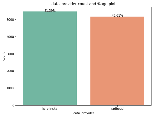
4.1 检查数据提供方分布
def plot_count(df, feature, title='', size=2):f, ax = plt.subplots(1,1, figsize=(4*size,3*size))total = float(len(df))sns.countplot(df[feature], order = df[feature].value_counts().index, palette='Set2')plt.title(title)for p in ax.patches:height = p.get_height()ax.text(p.get_x()+p.get_width()/2.,height + 3,'{:1.2f}%'.format(100*height/total),ha="center")plt.show()plot_count(df=train, feature='data_provider', title='数据提供方计数与百分比图')
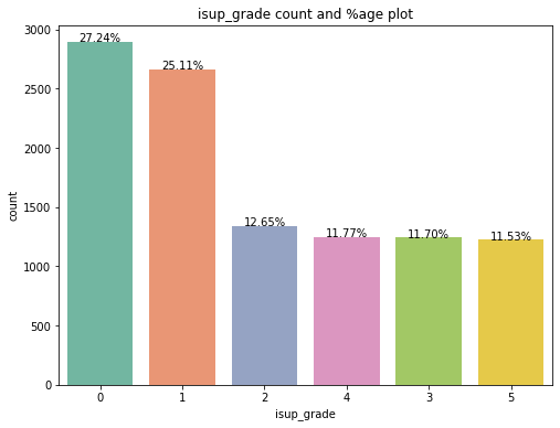
4.2 检查 ISUP 等级分布
python
plot_count(df=train, feature='isup_grade', title='ISUP等级计数与百分比图')
推论:
-
训练集中大部分样本的 ISUP 等级为 0 或 1(合计 > 50%)
-
其余样本的 ISUP 等级为 2 到 5,各约占 11-12%
-
数据集在 ISUP 等级上不平衡
4.3 检查格里森评分分布
python
plot_count(df=train, feature='gleason_score', title='格里森评分计数与百分比图', size=3)
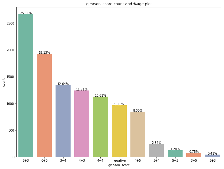
推论:
-
从上图可以清楚看到,格里森评分分布不均匀
-
部分格里森评分(如 3+3 和 0+0)出现频率较高,而其他(如 3+5 和 5+3)在此数据集中非常罕见
-
数据集在格里森评分上不平衡
4.4 检查 ISUP 等级与数据提供方的相对分布
def plot_relative_distribution(df, feature, hue, title='', size=2):f, ax = plt.subplots(1,1, figsize=(4*size,3*size))total = float(len(df))sns.countplot(x=feature, hue=hue, data=df, palette='Set2')plt.title(title)for p in ax.patches:height = p.get_height()ax.text(p.get_x()+p.get_width()/2.,height + 3,'{:1.2f}%'.format(100*height/total),ha="center")plt.show()plot_relative_distribution(df=train, feature='isup_grade', hue='data_provider',title='ISUP等级与数据提供方的相对计数图', size=2)
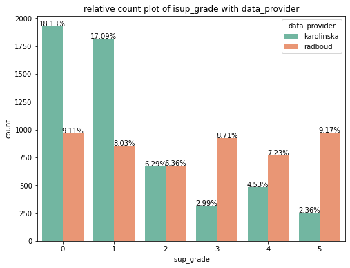
推论:
-
在 ISUP 等级 0 和 1 中,大部分数据由 karolinska 提供
-
在 ISUP 等级 3、4 和 5 中,大部分数据由 radboud 提供
4.5 检查格里森评分与数据提供方的相对分布
python
plot_relative_distribution(df=train, feature='gleason_score', hue='data_provider', title='格里森评分与数据提供方的相对计数图', size=3)
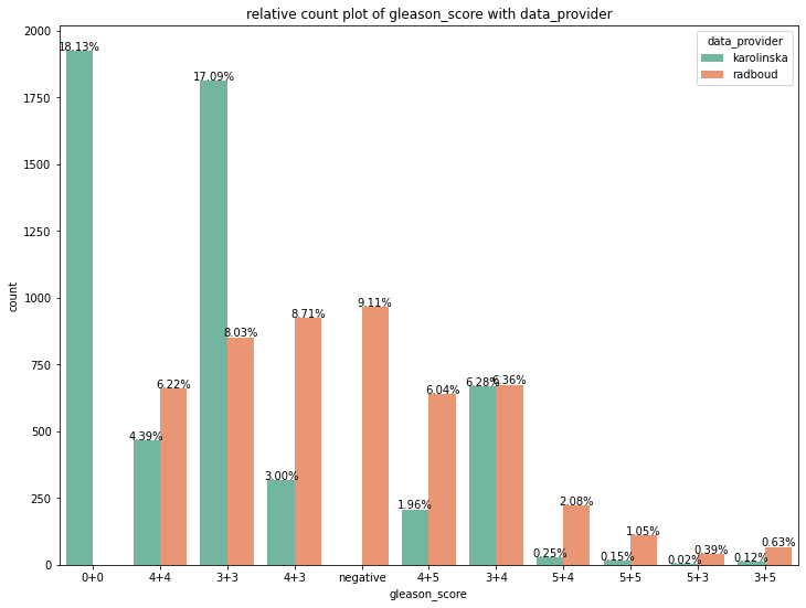
推论:
-
在格里森评分 (0+0) 类别中,所有数据由 karolinska 提供
-
在格里森评分 (negative) 类别中,所有数据由 radboud 提供
-
在格里森评分 (3+3) 类别中,karolinska 是主要数据提供方
-
另一方面,radboud 是 (4+4)、(4+3)、(4+5)、(5+4)、(5+5)、(5+3)、(3+5) 的主要数据提供方
4.6 检查 ISUP 等级与格里森评分的相对分布
python
plot_relative_distribution(df=train, feature='isup_grade', hue='gleason_score', title='ISUP等级与格里森评分的相对计数图', size=3)
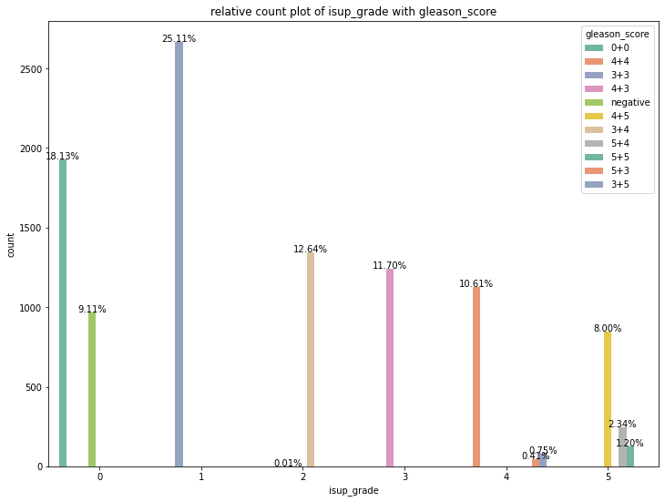
inference:
-
All exams with ISUP grade = 0 have Gleason score 0+0 or negative.
-
All exams with ISUP grade = 1 have Gleason score 3+3.
-
All exams with ISUP grade = 2 have Gleason score 3+4.
-
All exams with ISUP grade = 3 have Gleason score 4+3.
-
All exams with ISUP grade = 4 have Gleason score 4+4 (majority), 3+5 or 5+3.
-
All exams with ISUP grade = 5 have Gleason score 4+5 (majority), 5+4 or 5+5.
5. 快速显示几张图像
在接下来的部分中,我们将使用 OpenSlide 从切片中加载数据。使用 OpenSlide 的好处是,我们可以加载切片的任意区域,而无需将整张图像加载到内存中。想要交互式查看切片?我们在本笔记本的最后一节添加了一个交互式查看器。
您可以在文档中阅读更多关于 OpenSlide Python 绑定的信息:OpenSlide Python — OpenSlide Python 1.4.3 documentation
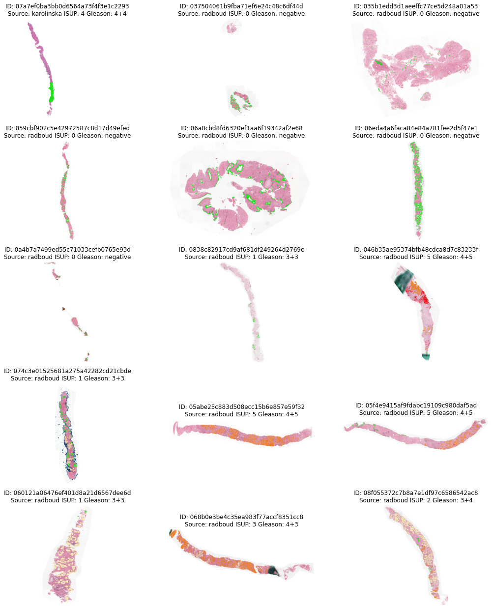
def display_images(slides):f, ax = plt.subplots(5,3, figsize=(18,22))for i, slide in enumerate(slides):image = openslide.OpenSlide(os.path.join(data_dir, f'{slide}.tiff'))spacing = 1 / (float(image.properties['tiff.XResolution']) / 10000)patch = image.read_region((1780,1950), 0, (256, 256))ax[i//3, i%3].imshow(patch)image.close()ax[i//3, i%3].axis('off')image_id = slidedata_provider = train.loc[slide, 'data_provider']isup_grade = train.loc[slide, 'isup_grade']gleason_score = train.loc[slide, 'gleason_score']ax[i//3, i%3].set_title(f"ID: {image_id}\n来源: {data_provider} ISUP: {isup_grade} 格里森: {gleason_score}")plt.show()# 15个图像ID列表images = [...] # 原列表保持不变display_images(images)
images = ['07a7ef0ba3bb0d6564a73f4f3e1c2293','037504061b9fba71ef6e24c48c6df44d','035b1edd3d1aeeffc77ce5d248a01a53','059cbf902c5e42972587c8d17d49efed','06a0cbd8fd6320ef1aa6f19342af2e68','06eda4a6faca84e84a781fee2d5f47e1','0a4b7a7499ed55c71033cefb0765e93d','0838c82917cd9af681df249264d2769c','046b35ae95374bfb48cdca8d7c83233f','074c3e01525681a275a42282cd21cbde','05abe25c883d508ecc15b6e857e59f32','05f4e9415af9fdabc19109c980daf5ad','060121a06476ef401d8a21d6567dee6d','068b0e3be4c35ea983f77accf8351cc8','08f055372c7b8a7e1df97c6586542ac8']display_images(images)
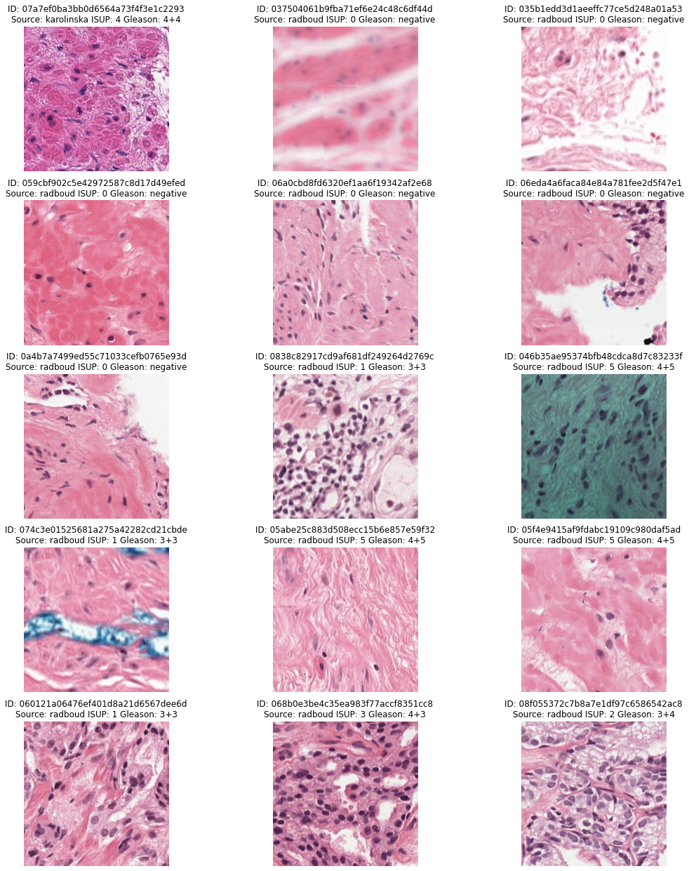
几点观察:
-
图像尺寸相当大(通常 x 和 y 方向都在 5,000 到 40,000 像素之间)
-
每个切片有 3 个可加载的层级,对应下采样倍率 1、4 和 16
-
每个层级的尺寸因原始图像尺寸而异
-
活检切片可能有不同的旋转角度。这种旋转没有临床价值,仅取决于实验室收集活检样本的方式
-
不同活检切片之间存在明显的颜色差异,这在病理学中非常常见,是由不同的实验室操作流程引起的
6. 加载标签掩码
除了切片级别的标签(存在于 CSV 文件中)外,训练集中几乎所有切片都有与之关联的掩码,提供额外的标签信息。这些掩码直接指示组织的哪些部分是健康的,哪些是癌变的。两个中心的掩码信息有所不同:
Radboudumc(拉德堡德大学医学中心):
前列腺腺体被单独标记。有效值为:
-
0:背景(非组织)或未知
-
1:间质(结缔组织,非上皮组织)
-
2:健康(良性)上皮
-
3:癌性上皮(格里森 3 型)
-
4:癌性上皮(格里森 4 型)
-
5:癌性上皮(格里森 5 型)
Karolinska(卡罗林斯卡学院):
区域被标记。有效值为:
-
0:背景(非组织)或未知
-
1:良性组织(间质和上皮合并)
-
2:癌性组织(间质和上皮合并)
Radboudumc 的标签掩码是由多个深度学习算法半自动生成的,包含噪声,可视为弱监督标签。Karolinska 的标签掩码基于病理学家的注释半自动生成。
标签掩码以 RGB 格式存储,便于图像阅读器打开。标签信息存储在红色(R)通道中,其他通道设置为零,可以忽略。与切片本身一样,标签掩码可以使用 OpenSlide 打开。
使用 matplotlib 可视化掩码
由于掩码只是整数矩阵,您也可以使用其他包来显示掩码。例如,使用 matplotlib 和自定义颜色映射,我们可以快速可视化不同的癌症区域:
def display_masks(slides):f, ax = plt.subplots(5,3, figsize=(18,22))for i, slide in enumerate(slides):mask = openslide.OpenSlide(os.path.join(mask_dir, f'{slide}_mask.tiff'))mask_data = mask.read_region((0,0), mask.level_count - 1, mask.level_dimensions[-1])cmap = matplotlib.colors.ListedColormap(['黑色', '灰色', '绿色', '黄色', '橙色', '红色'])ax[i//3, i%3].imshow(np.asarray(mask_data)[:,:,0], cmap=cmap, interpolation='nearest', vmin=0, vmax=5)mask.close()ax[i//3, i%3].axis('off')image_id = slidedata_provider = train.loc[slide, 'data_provider']isup_grade = train.loc[slide, 'isup_grade']gleason_score = train.loc[slide, 'gleason_score']ax[i//3, i%3].set_title(f"ID: {image_id}\n来源: {data_provider} ISUP: {isup_grade} 格里森: {gleason_score}")f.tight_layout()plt.show()display_masks(images)
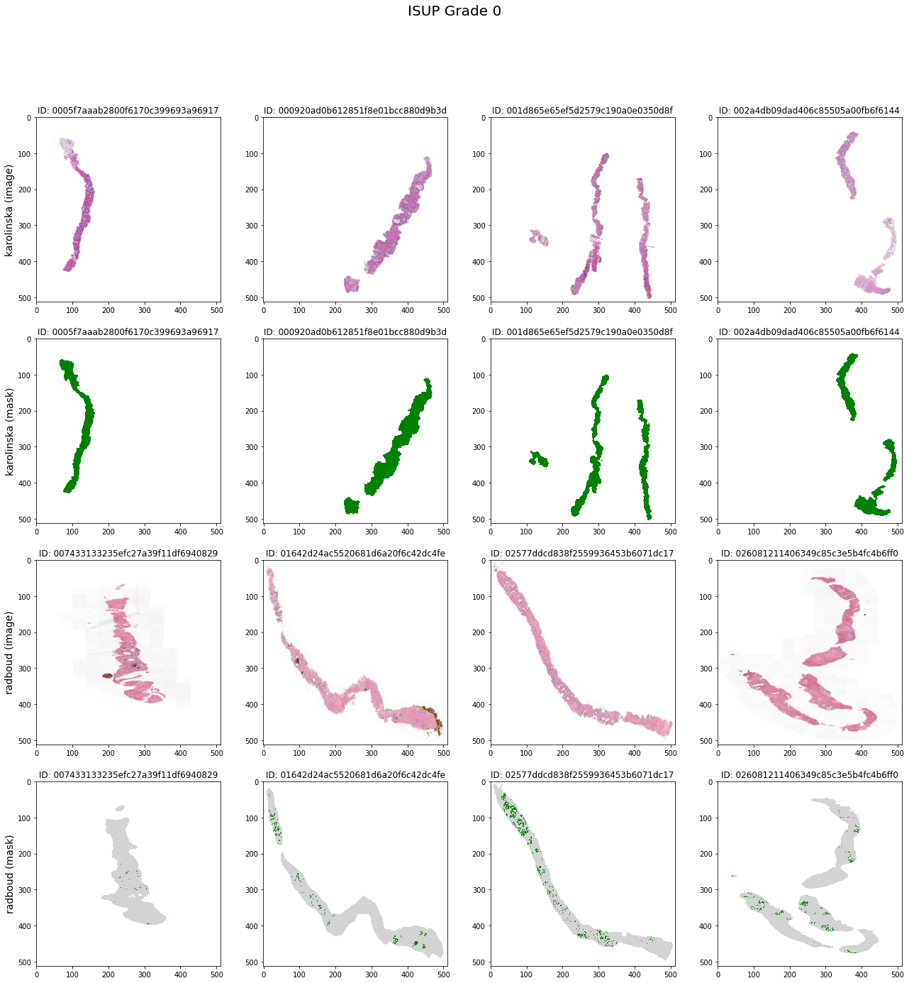
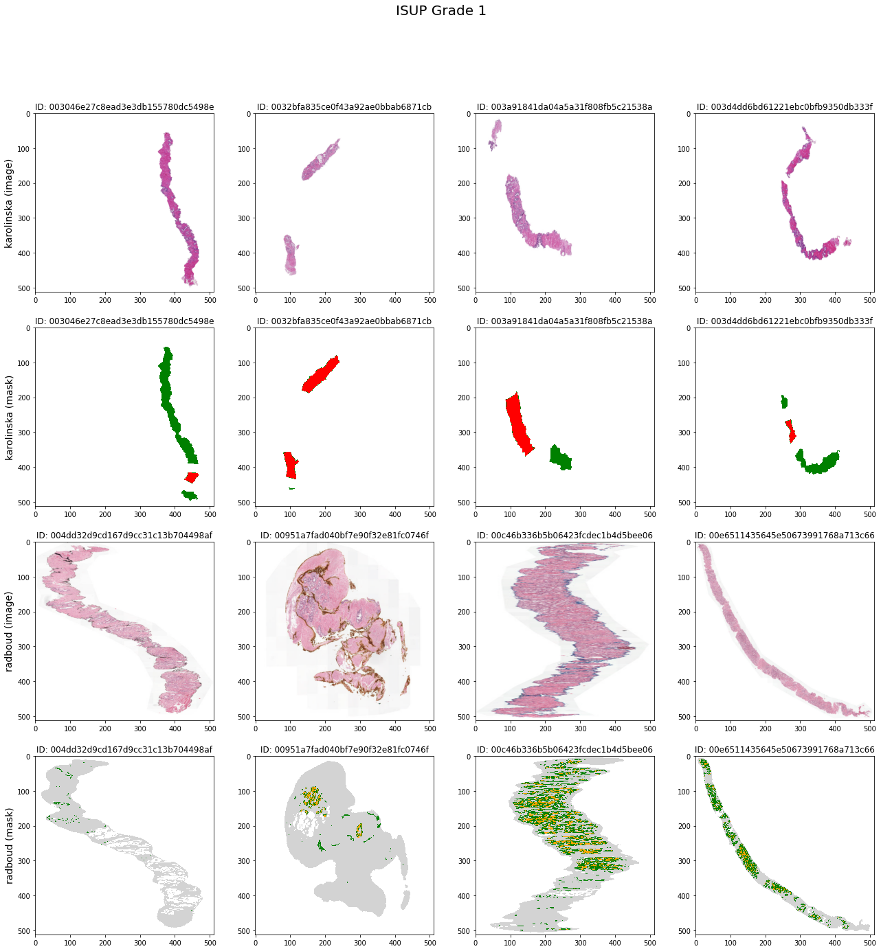
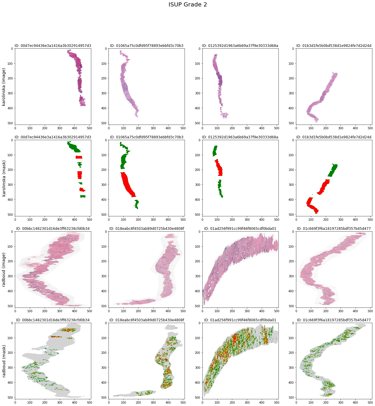
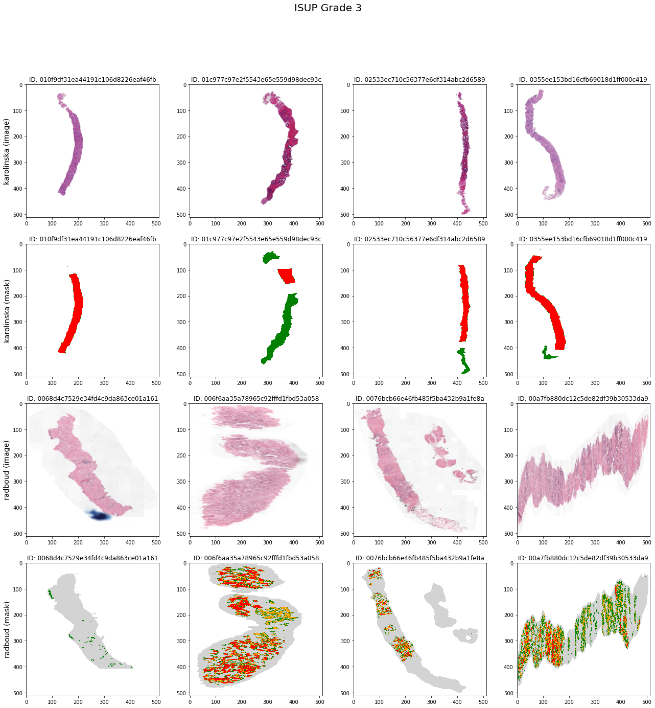
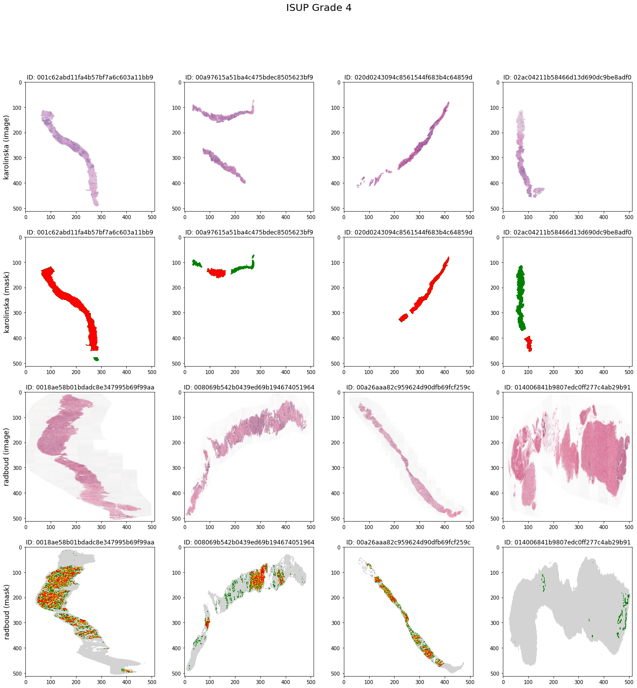
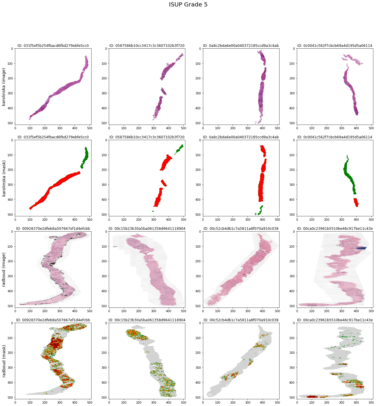
def load_and_resize_image(img_id):"""加载并调整图像大小"""biopsy = skimage.io.MultiImage(os.path.join(data_dir, f'{img_id}.tiff'))return cv2.resize(biopsy[-1], (512, 512))def load_and_resize_mask(img_id):"""加载并调整掩码大小"""biopsy = skimage.io.MultiImage(os.path.join(mask_dir, f'{img_id}_mask.tiff'))return cv2.resize(biopsy[-1], (512, 512))[:,:,0]# 按 ISUP 等级遍历,显示每个等级的图像和掩码for grade in range(train.isup_grade.nunique()):# ... 显示每个等级的 4x4 网格图像
显示每个 ISUP 等级类别的图像和掩码
从讨论线程中可以知道,掩码目录中有 100 张图像没有掩码。
labels = []for grade in range(train.isup_grade.nunique()):fig, ax = plt.subplots(nrows=4, ncols=4, figsize=(22, 22))for i, row in enumerate(ax):idx = i//2temp = train_df[(train_df.isup_grade == grade) & (train_df.data_provider == data_providers[idx])].image_id.head(4).reset_index(drop=True)if i%2 < 1:labels.append(f'{data_providers[idx]} (image)')for j, col in enumerate(row):col.imshow(load_and_resize_image(temp[j]))col.set_title(f"ID: {temp[j]}")else:labels.append(f'{data_providers[idx]} (mask)')for j, col in enumerate(row):if data_providers[idx] == 'radboud':col.imshow(load_and_resize_mask(temp[j]),cmap = matplotlib.colors.ListedColormap(['white', 'lightgrey', 'green', 'orange', 'red', 'darkred']),norm = matplotlib.colors.Normalize(vmin=0, vmax=5, clip=True))else:col.imshow(load_and_resize_mask(temp[j]),cmap = matplotlib.colors.ListedColormap(['white', 'green', 'red']),norm = matplotlib.colors.Normalize(vmin=0, vmax=2, clip=True))gleason_score = train.loc[temp[j], 'gleason_score']col.set_title(f"ID: {temp[j]}")for row, r in zip(ax[:,0], labels):row.set_ylabel(r, rotation=90, size='large', fontsize=14)plt.suptitle(f'ISUP Grade {grade}', fontsize=20)plt.show()
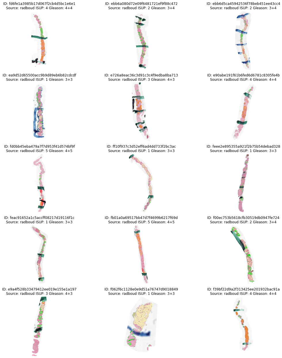
注意: 在下面的示例中,您还可以观察到切片上的一些笔迹标记(深绿色污迹)。这些标记不是组织的一部分,而是最初检查该病例的病理学家留下的。训练集中的一些切片上有这些笔迹标记。
探索带有笔迹标记的图像
训练数据集中有一些带有笔迹标记的图像。组织者留下了如下说明:
请注意,测试集图像的处理流程与训练集略有不同。部分训练集图像上有零星的笔迹标记,但测试集切片没有笔迹标记。
python
pen_marked_images =['fd6fe1a3985b17d067f2cb4d5bc1e6e1',# ... 其他14个ID]overlay_mask_on_slide(pen_marked_images)
7. 简单基线模型
Overlaying masks on the slides
As the masks have the same dimension as the slides, we can overlay the masks on the tissue to directly see which areas are cancerous. This overlay can help you identifying the different growth patterns. To do this, we load both the mask and the biopsy and merge them using PIL.
Tip: Want to view the slides in a more interactive way? Using a WSI viewer you can interactively view the slides. Examples of open source viewers that can open the PANDA dataset are ASAP and QuPath. ASAP can also overlay the masks on top of the images using the "Overlay" functionality. If you use Qupath, and the images do not load, try changing the file extension to .vtif.
def overlay_mask_on_slide(images, center='radboud', alpha=0.8, max_size=(800, 800)):"""Show a mask overlayed on a slide."""f, ax = plt.subplots(5,3, figsize=(18,22))for i, image_id in enumerate(images):slide = openslide.OpenSlide(os.path.join(data_dir, f'{image_id}.tiff'))mask = openslide.OpenSlide(os.path.join(mask_dir, f'{image_id}_mask.tiff'))slide_data = slide.read_region((0,0), slide.level_count - 1, slide.level_dimensions[-1])mask_data = mask.read_region((0,0), mask.level_count - 1, mask.level_dimensions[-1])mask_data = mask_data.split()[0]# Create alpha maskalpha_int = int(round(255*alpha))if center == 'radboud':alpha_content = np.less(mask_data.split()[0], 2).astype('uint8') * alpha_int + (255 - alpha_int)elif center == 'karolinska':alpha_content = np.less(mask_data.split()[0], 1).astype('uint8') * alpha_int + (255 - alpha_int)alpha_content = PIL.Image.fromarray(alpha_content)preview_palette = np.zeros(shape=768, dtype=int)if center == 'radboud':# Mapping: {0: background, 1: stroma, 2: benign epithelium, 3: Gleason 3, 4: Gleason 4, 5: Gleason 5}preview_palette[0:18] = (np.array([0, 0, 0, 0.5, 0.5, 0.5, 0, 1, 0, 1, 1, 0.7, 1, 0.5, 0, 1, 0, 0]) * 255).astype(int)elif center == 'karolinska':# Mapping: {0: background, 1: benign, 2: cancer}preview_palette[0:9] = (np.array([0, 0, 0, 0, 1, 0, 1, 0, 0]) * 255).astype(int)mask_data.putpalette(data=preview_palette.tolist())mask_rgb = mask_data.convert(mode='RGB')overlayed_image = PIL.Image.composite(image1=slide_data, image2=mask_rgb, mask=alpha_content)overlayed_image.thumbnail(size=max_size, resample=0)ax[i//3, i%3].imshow(overlayed_image)slide.close()mask.close()ax[i//3, i%3].axis('off')data_provider = train.loc[image_id, 'data_provider']isup_grade = train.loc[image_id, 'isup_grade']gleason_score = train.loc[image_id, 'gleason_score']ax[i//3, i%3].set_title(f"ID: {image_id}\nSource: {data_provider} ISUP: {isup_grade} Gleason: {gleason_score}")
Exploring images with pen markers
It is mentioned here that in training dataset, there are few images with pen markers on them. The organizers left us with a Note as described below.
Note that slightly different procedures were in place for the images used in the test set than the training set. Some of the training set images have stray pen marks on them, but the test set slides are free of pen marks.
Let's take a look on few of these images.
pen_marked_images = ['fd6fe1a3985b17d067f2cb4d5bc1e6e1','ebb6a080d72e09f6481721ef9f88c472','ebb6d5ca45942536f78beb451ee43cc4','ea9d52d65500acc9b9d89eb6b82cdcdf','e726a8eac36c3d91c3c4f9edba8ba713','e90abe191f61b6fed6d6781c8305fe4b','fd0bb45eba479a7f7d953f41d574bf9f','ff10f937c3d52eff6ad4dd733f2bc3ac','feee2e895355a921f2b75b54debad328','feac91652a1c5accff08217d19116f1c','fb01a0a69517bb47d7f4699b6217f69d','f00ec753b5618cfb30519db0947fe724','e9a4f528b33479412ee019e155e1a197','f062f6c1128e0e9d51a76747d9018849','f39bf22d9a2f313425ee201932bac91a',]overlay_mask_on_slide(pen_marked_images)
参考资料
参考内核:
领域知识来源:

AtomGit 是由开放原子开源基金会联合 CSDN 等生态伙伴共同推出的新一代开源与人工智能协作平台。平台坚持“开放、中立、公益”的理念,把代码托管、模型共享、数据集托管、智能体开发体验和算力服务整合在一起,为开发者提供从开发、训练到部署的一站式体验。
更多推荐



 9
9 0
0- 0


 已为社区贡献5条内容

所有评论(0)