主题062：结构动力学模型修正

1. 概述

1.1 模型修正的意义

结构动力学模型修正是指利用实测的模态参数（固有频率、阻尼比、模态振型）或响应数据，通过数学方法调整有限元模型的物理参数（质量、刚度、阻尼），使模型预测结果与实测数据一致的过程。模型修正是连接理论模型与实际结构的重要桥梁。

模型修正的主要目标：

• 提高模型精度：使有限元模型更准确地反映实际结构的动力学特性
• 损伤识别：通过模型参数变化识别结构损伤位置和程度
• 响应预测：基于修正后的模型进行更准确的动态响应预测
• 优化设计：为结构优化设计提供准确的分析模型
  
  
  
  
  
  
  

1.2 模型修正的基本原理

模型修正问题可以表述为优化问题：

$$\underset{\mathbf{p}}{\min }J(\mathbf{p})=\Vert {\mathbf{z}}_{exp}-\mathbf{z}(\mathbf{p}){\Vert }^2$$

其中：

• $\mathbf{p}$：待修正的模型参数
• ${\mathbf{z}}_{exp}$：实测数据（频率、振型等）
• $\mathbf{z}(\mathbf{p})$：模型预测数据
• $J(\mathbf{p})$：目标函数

约束条件：

• 参数物理意义约束：${\mathbf{p}}_{min}\le \mathbf{p}\le {\mathbf{p}}_{max}$
• 正定性约束：$\mathbf{K}(\mathbf{p})>0$，$\mathbf{M}(\mathbf{p})>0$

1.3 模型修正方法分类

1. 直接方法

• 基于矩阵的修正方法
• 基于特征方程的修正方法

2. 迭代方法

• 基于灵敏度分析的修正方法
• 基于优化算法的修正方法

3. 代理模型方法

• 响应面方法
• 神经网络方法
• Kriging方法

2. 理论基础

2.1 灵敏度分析方法

2.1.1 特征值灵敏度

特征值对设计参数的灵敏度：

$$\frac{\partial {\lambda }_i}{\partial p_j}=\frac{{\mathbf{\varphi }}_i^T\left(\frac{\partial \mathbf{K}}{\partial p_j}-{\lambda }_i\frac{\partial \mathbf{M}}{\partial p_j}\right){\mathbf{\varphi }}_i}{{\mathbf{\varphi }}_i^T\mathbf{M}{\mathbf{\varphi }}_i}$$

其中：

• ${\lambda }_i={\omega }_i^2$：第i阶特征值
• ${\mathbf{\varphi }}_i$：第i阶模态振型
• $p_j$：第j个设计参数

2.1.2 特征向量灵敏度

特征向量对设计参数的灵敏度：

$$\frac{\partial {\mathbf{\varphi }}_i}{\partial p_j}=\sum _{k=1,k\ne i}^n\frac{{\mathbf{\varphi }}_k^T\left(\frac{\partial \mathbf{K}}{\partial p_j}-{\lambda }_i\frac{\partial \mathbf{M}}{\partial p_j}\right){\mathbf{\varphi }}_i}{({\lambda }_i-{\lambda }_k){\mathbf{\varphi }}_k^T\mathbf{M}{\mathbf{\varphi }}_k}{\mathbf{\varphi }}_k$$

2.1.3 灵敏度矩阵

灵敏度矩阵建立了参数变化与模态参数变化之间的关系：

$$\mathbf{S}=\left[\begin{array}{ccc}\frac{\partial {\omega }_1}{\partial p_1}& \cdots & \frac{\partial {\omega }_1}{\partial p_m}\\ ⋮& \ddots & ⋮\\ \frac{\partial {\omega }_n}{\partial p_1}& \cdots & \frac{\partial {\omega }_n}{\partial p_m}\\ \frac{\partial {\varphi }_{11}}{\partial p_1}& \cdots & \frac{\partial {\varphi }_{11}}{\partial p_m}\\ ⋮& \ddots & ⋮\end{array}\right]$$

2.2 基于灵敏度分析的模型修正

2.2.1 线性修正方程

利用灵敏度矩阵，建立线性修正方程：

$$\Delta \mathbf{z}=\mathbf{S}\Delta \mathbf{p}$$

其中：

• $\Delta \mathbf{z}={\mathbf{z}}_{exp}-{\mathbf{z}}_{ana}$：残差向量
• $\Delta \mathbf{p}$：参数修正量

2.2.2 最小二乘解

当灵敏度矩阵不是方阵时，采用最小二乘法求解：

$$\Delta \mathbf{p}=({\mathbf{S}}^T\mathbf{S}{)}^{-1}{\mathbf{S}}^T\Delta \mathbf{z}$$

2.2.3 加权最小二乘

考虑不同测量数据的可靠性差异：

$$\Delta \mathbf{p}=({\mathbf{S}}^T\mathbf{WS}{)}^{-1}{\mathbf{S}}^T\mathbf{W}\Delta \mathbf{z}$$

其中，$\mathbf{W}$为权重矩阵。

2.2.4 迭代修正算法

1. 初始化参数 p₀
2. 计算当前模态参数 z(pₖ)
3. 计算残差 Δz = z_exp - z(pₖ)
4. 计算灵敏度矩阵 S
5. 求解修正量 Δp
6. 更新参数 pₖ₊₁ = pₖ + α·Δp
7. 检查收敛条件
8. 若不收敛，返回步骤2

2.3 基于特征方程的模型修正

2.3.1 矩阵修正方法

直接修正刚度矩阵和质量矩阵：

$$(\mathbf{K}+\Delta \mathbf{K}){\mathbf{\varphi }}_i={\lambda }_i(\mathbf{M}+\Delta \mathbf{M}){\mathbf{\varphi }}_i$$

2.3.2 最小秩修正

寻找最小秩的矩阵修正：

$$\min \text{rank}(\Delta \mathbf{K})$$

约束条件：
$$(\mathbf{K}+\Delta \mathbf{K})\mathbf{\Phi }=\mathbf{M}\mathbf{\Phi }\mathbf{\Lambda }$$

2.3.3 最优矩阵修正

考虑矩阵的对称性和稀疏性：

$$\underset{\Delta \mathbf{K}}{\min }\Vert \Delta \mathbf{K}{\Vert }_F$$

约束条件：

• $(\mathbf{K}+\Delta \mathbf{K})\mathbf{\Phi }=\mathbf{M}\mathbf{\Phi }\mathbf{\Lambda }$
• $\Delta \mathbf{K}=\Delta {\mathbf{K}}^T$
• 保持原有零元素位置

2.4 基于响应面的模型修正

2.4.1 响应面方法

用多项式函数近似模型响应与参数之间的关系：

$$z_i(\mathbf{p})\approx a_0+\sum _{j=1}^m{a}_j{p}_j+\sum _{j=1}^m\sum _{k=j}^m{b}_{jk}{p}_j{p}_k$$

2.4.2 试验设计

选择合适的样本点构建响应面：

• 全因子设计
• 中心复合设计
• Box-Behnken设计
• 拉丁超立方采样

2.4.3 响应面优化

基于响应面进行优化：

$$\underset{\mathbf{p}}{\min }\Vert {\mathbf{z}}_{exp}-{\mathbf{z}}_{RSM}(\mathbf{p}){\Vert }^2$$

2.5 基于优化算法的模型修正

2.5.1 目标函数

常用的目标函数形式：

频率残差：
$$J_f=\sum _{i=1}^n{w}_i^f{\left(\frac{f_i^{exp}-f_i(\mathbf{p})}{f_i^{exp}}\right)}^2$$

振型残差（MAC）：
$$J_{\varphi }=\sum _{i=1}^n{w}_i^{\varphi }(1-MAC({\mathbf{\varphi }}_i^{exp},{\mathbf{\varphi }}_i(\mathbf{p})){)}^2$$

综合目标函数：
$$J=J_f+J_{\varphi }$$

2.5.2 优化算法

梯度类算法：

• 最速下降法
• 共轭梯度法
• 拟牛顿法（BFGS）

启发式算法：

• 遗传算法（GA）
• 粒子群优化（PSO）
• 模拟退火（SA）

3. 案例分析

3.1 案例1：基于灵敏度分析的模型修正

问题描述：
利用灵敏度分析方法修正简支梁有限元模型的刚度参数，使模型预测的固有频率与实测频率一致。

Python代码实现：

import numpy as np
import matplotlib.pyplot as plt
from matplotlib.animation import FuncAnimation
import matplotlib
matplotlib.use('Agg')
plt.rcParams['font.sans-serif'] = ['SimHei']
plt.rcParams['axes.unicode_minus'] = False
from scipy.linalg import eigh, pinv

class BeamModel:
    """简支梁有限元模型"""
    
    def __init__(self, L, EI, rhoA, n_elements=10):
        self.L = L
        self.EI_base = EI
        self.rhoA = rhoA
        self.n_elements = n_elements
        self.le = L / n_elements
        self.K_base, self.M = self._build_matrices()
        self.EI = EI * np.ones(n_elements)  # 每个单元的刚度修正系数
    
    def _build_matrices(self):
        """建立刚度和质量矩阵"""
        n_nodes = self.n_elements + 1
        n_dof = 2 * n_nodes
        
        K = np.zeros((n_dof, n_dof))
        M = np.zeros((n_dof, n_dof))
        
        k_e = self.EI_base / self.le**3 * np.array([
            [12, 6*self.le, -12, 6*self.le],
            [6*self.le, 4*self.le**2, -6*self.le, 2*self.le**2],
            [-12, -6*self.le, 12, -6*self.le],
            [6*self.le, 2*self.le**2, -6*self.le, 4*self.le**2]
        ])
        
        m_e = self.rhoA * self.le / 420 * np.array([
            [156, 22*self.le, 54, -13*self.le],
            [22*self.le, 4*self.le**2, 13*self.le, -3*self.le**2],
            [54, 13*self.le, 156, -22*self.le],
            [-13*self.le, -3*self.le**2, -22*self.le, 4*self.le**2]
        ])
        
        for i in range(self.n_elements):
            dof = [2*i, 2*i+1, 2*i+2, 2*i+3]
            for ii in range(4):
                for jj in range(4):
                    K[dof[ii], dof[jj]] += k_e[ii, jj]
                    M[dof[ii], dof[jj]] += m_e[ii, jj]
        
        return K, M
    
    def get_system_matrices(self):
        """获取考虑修正的系统矩阵"""
        K = np.zeros_like(self.K_base)
        for i in range(self.n_elements):
            dof = [2*i, 2*i+1, 2*i+2, 2*i+3]
            k_e = self.EI[i] / self.EI_base
            for ii in range(4):
                for jj in range(4):
                    K[dof[ii], dof[jj]] += k_e * self.K_base[dof[ii], dof[jj]]
        return K, self.M
    
    def solve_modal(self, n_modes=5):
        """求解模态参数"""
        K, M = self.get_system_matrices()
        
        bc_dofs = [0, -2]
        free_dofs = [i for i in range(K.shape[0]) if i not in bc_dofs]
        
        K_reduced = K[np.ix_(free_dofs, free_dofs)]
        M_reduced = M[np.ix_(free_dofs, free_dofs)]
        
        eigenvalues, eigenvectors = eigh(K_reduced, M_reduced)
        eigenvalues = np.maximum(eigenvalues, 1e-10)
        frequencies = np.sqrt(eigenvalues) / (2 * np.pi)
        
        mode_shapes = np.zeros((K.shape[0], n_modes))
        for i in range(n_modes):
            mode_shapes[free_dofs, i] = eigenvectors[:, i]
            mode_shapes[:, i] /= np.max(np.abs(mode_shapes[:, i]))
        
        return frequencies[:n_modes], mode_shapes[:, :n_modes]

class SensitivityBasedUpdating:
    """基于灵敏度分析的模型修正"""
    
    def __init__(self, model):
        self.model = model
        self.history = {'parameters': [], 'frequencies': [], 'residuals': []}
    
    def compute_sensitivity_matrix(self, n_modes=3, delta=1e-6):
        """
        计算灵敏度矩阵
        
        Parameters:
        -----------
        n_modes : int
            考虑的模态数
        delta : float
            差分步长
        
        Returns:
        --------
        S : array
            灵敏度矩阵 (n_modes × n_parameters)
        """
        f0, _ = self.model.solve_modal(n_modes)
        n_params = self.model.n_elements
        
        S = np.zeros((n_modes, n_params))
        
        for j in range(n_params):
            # 正向扰动
            self.model.EI[j] += delta
            f_plus, _ = self.model.solve_modal(n_modes)
            
            # 负向扰动
            self.model.EI[j] -= 2 * delta
            f_minus, _ = self.model.solve_modal(n_modes)
            
            # 中心差分
            S[:, j] = (f_plus - f_minus) / (2 * delta)
            
            # 恢复原值
            self.model.EI[j] += delta
        
        return S
    
    def update_model(self, target_frequencies, n_iterations=20, alpha=0.5, tol=1e-6):
        """
        修正模型参数
        
        Parameters:
        -----------
        target_frequencies : array
            目标频率
        n_iterations : int
            最大迭代次数
        alpha : float
            步长因子
        tol : float
            收敛容差
        
        Returns:
        --------
        success : bool
            是否收敛
        """
        n_modes = len(target_frequencies)
        
        for iteration in range(n_iterations):
            # 计算当前频率
            f_current, _ = self.model.solve_modal(n_modes)
            
            # 计算残差
            residual = target_frequencies - f_current
            residual_norm = np.linalg.norm(residual)
            
            # 记录历史
            self.history['parameters'].append(self.model.EI.copy())
            self.history['frequencies'].append(f_current.copy())
            self.history['residuals'].append(residual_norm)
            
            print(f"  迭代 {iteration+1}: 残差 = {residual_norm:.6f}")
            
            # 检查收敛
            if residual_norm < tol:
                print(f"  收敛！")
                return True
            
            # 计算灵敏度矩阵
            S = self.compute_sensitivity_matrix(n_modes)
            
            # 求解修正量（最小二乘）
            try:
                delta_p = pinv(S) @ residual
            except:
                delta_p = np.linalg.lstsq(S, residual, rcond=None)[0]
            
            # 更新参数
            self.model.EI += alpha * delta_p
            
            # 确保参数为正
            self.model.EI = np.maximum(self.model.EI, 0.1 * self.model.EI_base)
        
        print(f"  达到最大迭代次数")
        return False

def case1_sensitivity_updating():
    """案例1：基于灵敏度分析的模型修正"""
    print("="*60)
    print("主题062 - 案例1: 基于灵敏度分析的模型修正")
    print("="*60)
    
    # 创建模型
    L = 10.0
    EI = 2e8
    rhoA = 500
    n_elements = 10
    
    model = BeamModel(L, EI, rhoA, n_elements)
    
    # 获取"实测"频率（使用真实参数）
    f_true, modes_true = model.solve_modal(3)
    print("\n真实模态参数:")
    for i, f in enumerate(f_true):
        print(f"  第{i+1}阶频率: {f:.3f} Hz")
    
    # 引入误差（模拟不准确的初始模型）
    np.random.seed(42)
    error_factors = np.random.uniform(0.7, 1.3, n_elements)
    model.EI = EI * error_factors
    
    f_initial, _ = model.solve_modal(3)
    print("\n初始模型频率:")
    for i, f in enumerate(f_initial):
        print(f"  第{i+1}阶频率: {f:.3f} Hz (误差: {(f-f_true[i])/f_true[i]*100:.1f}%)")
    
    # 模型修正
    print("\n开始模型修正...")
    updater = SensitivityBasedUpdating(model)
    updater.update_model(f_true, n_iterations=15, alpha=0.3)
    
    # 修正后结果
    f_updated, _ = model.solve_modal(3)
    print("\n修正后模型频率:")
    for i, f in enumerate(f_updated):
        print(f"  第{i+1}阶频率: {f:.3f} Hz (误差: {(f-f_true[i])/f_true[i]*100:.1f}%)")
    
    # 可视化
    fig, axes = plt.subplots(2, 2, figsize=(14, 10))
    
    # 1. 参数收敛历史
    ax = axes[0, 0]
    param_history = np.array(updater.history['parameters']) / EI
    for i in range(n_elements):
        ax.plot(param_history[:, i], label=f'单元{i+1}', alpha=0.7)
    ax.axhline(y=1.0, color='red', linestyle='--', linewidth=2, label='真实值')
    ax.set_xlabel('迭代次数')
    ax.set_ylabel('刚度修正系数')
    ax.set_title('参数收敛历史')
    ax.legend(bbox_to_anchor=(1.05, 1), loc='upper left', fontsize=8)
    ax.grid(True, alpha=0.3)
    
    # 2. 频率收敛历史
    ax = axes[0, 1]
    freq_history = np.array(updater.history['frequencies'])
    for i in range(3):
        ax.plot(freq_history[:, i], label=f'第{i+1}阶', alpha=0.7)
        ax.axhline(y=f_true[i], color='red', linestyle='--', linewidth=1, alpha=0.5)
    ax.set_xlabel('迭代次数')
    ax.set_ylabel('频率 (Hz)')
    ax.set_title('频率收敛历史')
    ax.legend()
    ax.grid(True, alpha=0.3)
    
    # 3. 残差收敛
    ax = axes[1, 0]
    ax.semilogy(updater.history['residuals'], 'b-', linewidth=2)
    ax.set_xlabel('迭代次数')
    ax.set_ylabel('残差范数')
    ax.set_title('残差收敛曲线')
    ax.grid(True, alpha=0.3)
    
    # 4. 频率对比
    ax = axes[1, 1]
    x = np.arange(3)
    width = 0.25
    ax.bar(x - width, f_true, width, label='真实值', color='green', alpha=0.8)
    ax.bar(x, f_initial, width, label='初始模型', color='red', alpha=0.8)
    ax.bar(x + width, f_updated, width, label='修正后', color='blue', alpha=0.8)
    ax.set_xlabel('模态阶数')
    ax.set_ylabel('频率 (Hz)')
    ax.set_title('频率对比')
    ax.set_xticks(x)
    ax.set_xticklabels([f'第{i+1}阶' for i in range(3)])
    ax.legend()
    ax.grid(True, alpha=0.3, axis='y')
    
    plt.tight_layout()
    plt.savefig('sensitivity_updating.png', dpi=150, bbox_inches='tight')
    print("\n灵敏度分析模型修正图已保存: sensitivity_updating.png")
    plt.close()
    
    # 创建动画
    fig, axes = plt.subplots(1, 2, figsize=(14, 5))
    
    ax1 = axes[0]
    lines1 = []
    for i in range(n_elements):
        line, = ax1.plot([], [], label=f'单元{i+1}', alpha=0.7)
        lines1.append(line)
    ax1.set_xlim(0, len(updater.history['parameters']))
    ax1.set_ylim(0.5, 1.5)
    ax1.set_xlabel('迭代次数')
    ax1.set_ylabel('刚度修正系数')
    ax1.set_title('参数收敛动画')
    ax1.legend(bbox_to_anchor=(1.05, 1), loc='upper left', fontsize=8)
    ax1.grid(True, alpha=0.3)
    
    ax2 = axes[1]
    lines2 = []
    for i in range(3):
        line, = ax2.plot([], [], label=f'第{i+1}阶', alpha=0.7)
        lines2.append(line)
    ax2.set_xlim(0, len(updater.history['frequencies']))
    ax2.set_ylim(np.min(freq_history) * 0.9, np.max(freq_history) * 1.1)
    ax2.set_xlabel('迭代次数')
    ax2.set_ylabel('频率 (Hz)')
    ax2.set_title('频率收敛动画')
    ax2.legend()
    ax2.grid(True, alpha=0.3)
    
    def animate(frame):
        for i, line in enumerate(lines1):
            line.set_data(range(frame+1), param_history[:frame+1, i])
        
        for i, line in enumerate(lines2):
            line.set_data(range(frame+1), freq_history[:frame+1, i])
        
        return lines1 + lines2
    
    anim = FuncAnimation(fig, animate, frames=len(updater.history['parameters']), 
                         interval=300, blit=False)
    anim.save('sensitivity_animation.gif', writer='pillow', fps=3, dpi=100)
    print("灵敏度分析动画已保存: sensitivity_animation.gif")
    plt.close()
    
    return updater

if __name__ == "__main__":
    updater = case1_sensitivity_updating()

3.2 案例2：基于特征方程的模型修正

问题描述：
利用特征方程方法直接修正结构的质量矩阵和刚度矩阵，使修正后的矩阵满足实测的模态参数。

Python代码实现：

import numpy as np
import matplotlib.pyplot as plt
from matplotlib.animation import FuncAnimation
import matplotlib
matplotlib.use('Agg')
plt.rcParams['font.sans-serif'] = ['SimHei']
plt.rcParams['axes.unicode_minus'] = False
from scipy.linalg import eigh, svd, pinv

class EigenvalueBasedUpdating:
    """基于特征方程的模型修正"""
    
    def __init__(self, K_initial, M_initial):
        """
        初始化
        
        Parameters:
        -----------
        K_initial : array
            初始刚度矩阵
        M_initial : array
            初始质量矩阵
        """
        self.K0 = K_initial
        self.M0 = M_initial
        self.n_dof = K_initial.shape[0]
        self.history = {'K_error': [], 'M_error': [], 'eigenvalue_error': []}
    
    def update_matrix_direct(self, target_eigenvalues, target_eigenvectors, 
                             n_modes=None, alpha_K=0.5, alpha_M=0.5):
        """
        直接矩阵修正方法
        
        Parameters:
        -----------
        target_eigenvalues : array
            目标特征值
        target_eigenvectors : array
            目标特征向量
        n_modes : int
            使用的模态数
        alpha_K, alpha_M : float
            修正系数
        
        Returns:
        --------
        K_updated : array
            修正后的刚度矩阵
        M_updated : array
            修正后的质量矩阵
        """
        if n_modes is None:
            n_modes = len(target_eigenvalues)
        
        # 提取前n_modes阶模态
        Lambda_target = np.diag(target_eigenvalues[:n_modes])
        Phi_target = target_eigenvectors[:, :n_modes]
        
        # 计算当前模态
        eigenvalues, eigenvectors = eigh(self.K0, self.M0)
        Lambda_current = np.diag(eigenvalues[:n_modes])
        Phi_current = eigenvectors[:, :n_modes]
        
        # 刚度矩阵修正
        delta_K = alpha_K * (Phi_target @ Lambda_target @ Phi_target.T - 
                             Phi_current @ Lambda_current @ Phi_current.T)
        K_updated = self.K0 + delta_K
        
        # 质量矩阵修正
        delta_M = alpha_M * (Phi_target @ Phi_target.T - Phi_current @ Phi_current.T)
        M_updated = self.M0 + delta_M
        
        # 确保对称性
        K_updated = 0.5 * (K_updated + K_updated.T)
        M_updated = 0.5 * (M_updated + M_updated.T)
        
        return K_updated, M_updated
    
    def update_matrix_optimal(self, target_eigenvalues, target_eigenvectors,
                              n_modes=None, weight_K=1.0, weight_M=1.0):
        """
        最优矩阵修正方法
        
        Parameters:
        -----------
        target_eigenvalues : array
            目标特征值
        target_eigenvectors : array
            目标特征向量
        n_modes : int
            使用的模态数
        weight_K, weight_M : float
            权重系数
        
        Returns:
        --------
        K_updated : array
            修正后的刚度矩阵
        M_updated : array
            修正后的质量矩阵
        """
        if n_modes is None:
            n_modes = len(target_eigenvalues)
        
        # 提取前n_modes阶模态
        Lambda = np.diag(target_eigenvalues[:n_modes])
        Phi = target_eigenvectors[:, :n_modes]
        
        # 构建约束矩阵
        B_K = np.zeros((n_modes * self.n_dof, self.n_dof * self.n_dof))
        B_M = np.zeros((n_modes * self.n_dof, self.n_dof * self.n_dof))
        
        for i in range(n_modes):
            phi_i = Phi[:, i]
            lambda_i = target_eigenvalues[i]
            
            for j in range(self.n_dof):
                for k in range(self.n_dof):
                    idx = j * self.n_dof + k
                    B_K[i * self.n_dof + j, idx] = phi_i[k] * phi_i[j]
                    B_M[i * self.n_dof + j, idx] = lambda_i * phi_i[k] * phi_i[j]
        
        # 目标向量
        target_K = (Phi @ Lambda @ Phi.T).flatten()
        target_M = (Phi @ Phi.T).flatten()
        
        # 最小二乘求解
        K0_flat = self.K0.flatten()
        M0_flat = self.M0.flatten()
        
        # 修正量
        delta_K_flat = pinv(B_K) @ (target_K - B_K @ K0_flat)
        delta_M_flat = pinv(B_M) @ (target_M - B_M @ M0_flat)
        
        # 重构矩阵
        K_updated = self.K0 + weight_K * delta_K_flat.reshape(self.n_dof, self.n_dof)
        M_updated = self.M0 + weight_M * delta_M_flat.reshape(self.n_dof, self.n_dof)
        
        # 确保对称性和正定性
        K_updated = 0.5 * (K_updated + K_updated.T)
        M_updated = 0.5 * (M_updated + M_updated.T)
        
        # 添加正则化确保正定性
        K_updated += 1e-6 * np.eye(self.n_dof) * np.trace(K_updated) / self.n_dof
        M_updated += 1e-6 * np.eye(self.n_dof) * np.trace(M_updated) / self.n_dof
        
        return K_updated, M_updated
    
    def compute_error(self, K, M, target_eigenvalues, target_eigenvectors, n_modes=3):
        """计算误差"""
        eigenvalues, eigenvectors = eigh(K, M)
        
        # 特征值误差
        ev_error = np.linalg.norm(eigenvalues[:n_modes] - target_eigenvalues[:n_modes])
        
        # 矩阵误差（相对于真实矩阵）
        K_error = np.linalg.norm(K - self.K0) / np.linalg.norm(self.K0)
        M_error = np.linalg.norm(M - self.M0) / np.linalg.norm(self.M0)
        
        return ev_error, K_error, M_error

def create_mass_spring_system(n_dof=5, k_base=1000, m_base=1.0, 
                              k_error=0.2, m_error=0.1):
    """
    创建质量-弹簧系统
    
    Parameters:
    -----------
    n_dof : int
        自由度数量
    k_base : float
        基础刚度
    m_base : float
        基础质量
    k_error : float
        刚度误差比例
    m_error : float
        质量误差比例
    
    Returns:
    --------
    K_true, M_true : 真实矩阵
    K_initial, M_initial : 初始（有误差的）矩阵
    """
    # 真实刚度矩阵（三对角）
    K_true = np.zeros((n_dof, n_dof))
    for i in range(n_dof):
        if i > 0:
            K_true[i, i-1] = -k_base
            K_true[i-1, i] = -k_base
        K_true[i, i] = 2 * k_base
    K_true[0, 0] = k_base
    K_true[-1, -1] = k_base
    
    # 真实质量矩阵（对角）
    M_true = m_base * np.eye(n_dof)
    
    # 添加误差
    np.random.seed(42)
    K_perturb = np.random.uniform(-k_error, k_error, (n_dof, n_dof))
    M_perturb = np.random.uniform(-m_error, m_error, (n_dof, n_dof))
    
    K_initial = K_true * (1 + K_perturb)
    M_initial = M_true * (1 + np.diag(np.diag(M_perturb)))
    
    # 确保对称性
    K_initial = 0.5 * (K_initial + K_initial.T)
    
    return K_true, M_true, K_initial, M_initial

def case2_eigenvalue_updating():
    """案例2：基于特征方程的模型修正"""
    print("="*60)
    print("主题062 - 案例2: 基于特征方程的模型修正")
    print("="*60)
    
    # 创建系统
    n_dof = 5
    k_base = 1000
    m_base = 1.0
    
    K_true, M_true, K_initial, M_initial = create_mass_spring_system(
        n_dof, k_base, m_base, k_error=0.3, m_error=0.2
    )
    
    # 获取真实模态
    eigenvalues_true, eigenvectors_true = eigh(K_true, M_true)
    frequencies_true = np.sqrt(eigenvalues_true) / (2 * np.pi)
    
    print("\n真实模态参数:")
    for i in range(3):
        print(f"  第{i+1}阶: 频率 = {frequencies_true[i]:.3f} Hz")
    
    # 初始模态
    eigenvalues_initial, eigenvectors_initial = eigh(K_initial, M_initial)
    frequencies_initial = np.sqrt(eigenvalues_initial) / (2 * np.pi)
    
    print("\n初始模型模态:")
    for i in range(3):
        error = (frequencies_initial[i] - frequencies_true[i]) / frequencies_true[i] * 100
        print(f"  第{i+1}阶: 频率 = {frequencies_initial[i]:.3f} Hz (误差: {error:.1f}%)")
    
    # 模型修正
    print("\n开始模型修正...")
    updater = EigenvalueBasedUpdating(K_initial, M_initial)
    
    # 方法1：直接修正
    print("\n方法1: 直接矩阵修正")
    K_direct, M_direct = updater.update_matrix_direct(
        eigenvalues_true, eigenvectors_true, n_modes=3, alpha_K=0.8, alpha_M=0.8
    )
    
    eigenvalues_direct, eigenvectors_direct = eigh(K_direct, M_direct)
    frequencies_direct = np.sqrt(eigenvalues_direct) / (2 * np.pi)
    
    print("修正后模态:")
    for i in range(3):
        error = (frequencies_direct[i] - frequencies_true[i]) / frequencies_true[i] * 100
        print(f"  第{i+1}阶: 频率 = {frequencies_direct[i]:.3f} Hz (误差: {error:.1f}%)")
    
    # 方法2：最优修正
    print("\n方法2: 最优矩阵修正")
    K_optimal, M_optimal = updater.update_matrix_optimal(
        eigenvalues_true, eigenvectors_true, n_modes=3, weight_K=1.0, weight_M=1.0
    )
    
    eigenvalues_optimal, eigenvectors_optimal = eigh(K_optimal, M_optimal)
    frequencies_optimal = np.sqrt(eigenvalues_optimal) / (2 * np.pi)
    
    print("修正后模态:")
    for i in range(3):
        error = (frequencies_optimal[i] - frequencies_true[i]) / frequencies_true[i] * 100
        print(f"  第{i+1}阶: 频率 = {frequencies_optimal[i]:.3f} Hz (误差: {error:.1f}%)")
    
    # 可视化
    fig, axes = plt.subplots(2, 3, figsize=(15, 10))
    
    # 1. 刚度矩阵对比
    ax = axes[0, 0]
    im = ax.imshow(K_true, cmap='RdBu_r', aspect='auto')
    ax.set_title('真实刚度矩阵')
    ax.set_xlabel('自由度')
    ax.set_ylabel('自由度')
    plt.colorbar(im, ax=ax)
    
    ax = axes[0, 1]
    im = ax.imshow(K_initial, cmap='RdBu_r', aspect='auto')
    ax.set_title('初始刚度矩阵')
    ax.set_xlabel('自由度')
    ax.set_ylabel('自由度')
    plt.colorbar(im, ax=ax)
    
    ax = axes[0, 2]
    im = ax.imshow(K_optimal, cmap='RdBu_r', aspect='auto')
    ax.set_title('修正后刚度矩阵')
    ax.set_xlabel('自由度')
    ax.set_ylabel('自由度')
    plt.colorbar(im, ax=ax)
    
    # 2. 质量矩阵对比
    ax = axes[1, 0]
    im = ax.imshow(M_true, cmap='RdBu_r', aspect='auto')
    ax.set_title('真实质量矩阵')
    ax.set_xlabel('自由度')
    ax.set_ylabel('自由度')
    plt.colorbar(im, ax=ax)
    
    ax = axes[1, 1]
    im = ax.imshow(M_initial, cmap='RdBu_r', aspect='auto')
    ax.set_title('初始质量矩阵')
    ax.set_xlabel('自由度')
    ax.set_ylabel('自由度')
    plt.colorbar(im, ax=ax)
    
    ax = axes[1, 2]
    im = ax.imshow(M_optimal, cmap='RdBu_r', aspect='auto')
    ax.set_title('修正后质量矩阵')
    ax.set_xlabel('自由度')
    ax.set_ylabel('自由度')
    plt.colorbar(im, ax=ax)
    
    plt.tight_layout()
    plt.savefig('eigenvalue_updating.png', dpi=150, bbox_inches='tight')
    print("\n特征方程模型修正图已保存: eigenvalue_updating.png")
    plt.close()
    
    # 频率对比图
    fig, ax = plt.subplots(figsize=(10, 6))
    x = np.arange(n_dof)
    width = 0.2
    
    ax.bar(x - 1.5*width, frequencies_true, width, label='真实值', color='green', alpha=0.8)
    ax.bar(x - 0.5*width, frequencies_initial, width, label='初始模型', color='red', alpha=0.8)
    ax.bar(x + 0.5*width, frequencies_direct, width, label='直接修正', color='blue', alpha=0.8)
    ax.bar(x + 1.5*width, frequencies_optimal, width, label='最优修正', color='purple', alpha=0.8)
    
    ax.set_xlabel('模态阶数')
    ax.set_ylabel('频率 (Hz)')
    ax.set_title('频率对比')
    ax.set_xticks(x)
    ax.set_xticklabels([f'第{i+1}阶' for i in range(n_dof)])
    ax.legend()
    ax.grid(True, alpha=0.3, axis='y')
    
    plt.tight_layout()
    plt.savefig('frequency_comparison.png', dpi=150, bbox_inches='tight')
    print("频率对比图已保存: frequency_comparison.png")
    plt.close()
    
    return updater

if __name__ == "__main__":
    updater = case2_eigenvalue_updating()

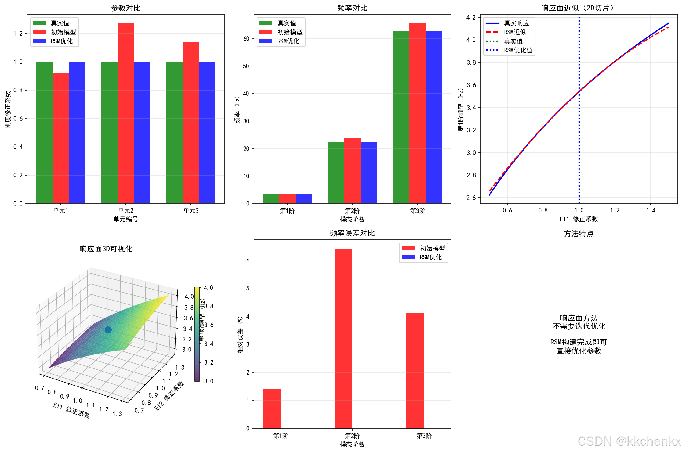
3.3 案例3：基于响应面的模型修正

问题描述：
利用响应面方法建立模型参数与模态参数之间的近似关系，通过优化响应面函数来修正模型参数。

Python代码实现：

import numpy as np
import matplotlib.pyplot as plt
from matplotlib.animation import FuncAnimation
from mpl_toolkits.mplot3d import Axes3D
import matplotlib
matplotlib.use('Agg')
plt.rcParams['font.sans-serif'] = ['SimHei']
plt.rcParams['axes.unicode_minus'] = False
from scipy.linalg import eigh
from scipy.optimize import minimize

class ResponseSurfaceModel:
    """响应面模型"""
    
    def __init__(self, n_params, n_responses):
        """
        初始化响应面模型
        
        Parameters:
        -----------
        n_params : int
            参数数量
        n_responses : int
            响应数量
        """
        self.n_params = n_params
        self.n_responses = n_responses
        self.coefficients = None
        self.X_mean = None
        self.X_std = None
        self.y_mean = None
        self.y_std = None
    
    def generate_samples(self, param_ranges, n_samples=50):
        """
        生成样本点（拉丁超立方采样）
        
        Parameters:
        -----------
        param_ranges : list
            参数范围列表 [(min1, max1), (min2, max2), ...]
        n_samples : int
            样本数量
        
        Returns:
        --------
        samples : array
            样本点 (n_samples × n_params)
        """
        samples = np.zeros((n_samples, self.n_params))
        
        for i in range(self.n_params):
            pmin, pmax = param_ranges[i]
            # 拉丁超立方采样
            cut = np.linspace(0, 1, n_samples + 1)
            u = np.random.rand(n_samples)
            samples[:, i] = pmin + (pmax - pmin) * (cut[:-1] + u * (cut[1] - cut[:-1]))
        
        return samples
    
    def fit(self, X, y):
        """
        拟合响应面（二次多项式）
        
        Parameters:
        -----------
        X : array
            输入样本 (n_samples × n_params)
        y : array
            输出响应 (n_samples × n_responses)
        """
        n_samples = X.shape[0]
        
        # 标准化
        self.X_mean = np.mean(X, axis=0)
        self.X_std = np.std(X, axis=0)
        self.y_mean = np.mean(y, axis=0)
        self.y_std = np.std(y, axis=0)
        
        X_norm = (X - self.X_mean) / (self.X_std + 1e-10)
        y_norm = (y - self.y_mean) / (self.y_std + 1e-10)
        
        # 构建设计矩阵（包含常数项、线性项和二次项）
        n_terms = 1 + self.n_params + self.n_params * (self.n_params + 1) // 2
        Phi = np.zeros((n_samples, n_terms))
        
        col = 0
        # 常数项
        Phi[:, col] = 1
        col += 1
        
        # 线性项
        for i in range(self.n_params):
            Phi[:, col] = X_norm[:, i]
            col += 1
        
        # 二次项（包括交叉项）
        for i in range(self.n_params):
            for j in range(i, self.n_params):
                Phi[:, col] = X_norm[:, i] * X_norm[:, j]
                col += 1
        
        # 最小二乘拟合
        self.coefficients = np.linalg.lstsq(Phi, y_norm, rcond=None)[0]
    
    def predict(self, X):
        """
        预测响应
        
        Parameters:
        -----------
        X : array
            输入参数 (n_samples × n_params)
        
        Returns:
        --------
        y_pred : array
            预测响应
        """
        n_samples = X.shape[0] if X.ndim > 1 else 1
        X = X.reshape(n_samples, self.n_params)
        
        # 标准化
        X_norm = (X - self.X_mean) / (self.X_std + 1e-10)
        
        # 构建设计矩阵
        n_terms = 1 + self.n_params + self.n_params * (self.n_params + 1) // 2
        Phi = np.zeros((n_samples, n_terms))
        
        col = 0
        Phi[:, col] = 1
        col += 1
        
        for i in range(self.n_params):
            Phi[:, col] = X_norm[:, i]
            col += 1
        
        for i in range(self.n_params):
            for j in range(i, self.n_params):
                Phi[:, col] = X_norm[:, i] * X_norm[:, j]
                col += 1
        
        # 预测并反标准化
        y_pred_norm = Phi @ self.coefficients
        y_pred = y_pred_norm * (self.y_std + 1e-10) + self.y_mean
        
        return y_pred

class RSMModelUpdating:
    """基于响应面的模型修正"""
    
    def __init__(self, model_func):
        """
        初始化
        
        Parameters:
        -----------
        model_func : callable
            模型函数，输入参数，输出频率
        """
        self.model_func = model_func
        self.rsm = None
        self.history = {'params': [], 'errors': []}
    
    def build_response_surface(self, param_ranges, n_samples=50):
        """
        构建响应面
        
        Parameters:
        -----------
        param_ranges : list
            参数范围
        n_samples : int
            样本数量
        """
        n_params = len(param_ranges)
        
        # 生成样本
        rsm_temp = ResponseSurfaceModel(n_params, 1)
        X_samples = rsm_temp.generate_samples(param_ranges, n_samples)
        
        # 计算响应
        y_samples = np.zeros((n_samples, 3))  # 假设有3阶频率
        for i in range(n_samples):
            freqs = self.model_func(X_samples[i])
            y_samples[i, :len(freqs)] = freqs[:3]
        
        # 为每个响应构建响应面
        self.rsm = []
        for j in range(3):
            rsm = ResponseSurfaceModel(n_params, 1)
            rsm.fit(X_samples, y_samples[:, j:j+1])
            self.rsm.append(rsm)
    
    def optimize_parameters(self, target_frequencies, param_ranges, method='SLSQP'):
        """
        优化参数
        
        Parameters:
        -----------
        target_frequencies : array
            目标频率
        param_ranges : list
            参数范围
        method : str
            优化方法
        
        Returns:
        --------
        optimal_params : array
            最优参数
        """
        n_params = len(param_ranges)
        
        # 目标函数
        def objective(p):
            error = 0
            for i, rsm in enumerate(self.rsm[:len(target_frequencies)]):
                f_pred = rsm.predict(p.reshape(1, -1))[0, 0]
                error += ((f_pred - target_frequencies[i]) / target_frequencies[i])**2
            return error
        
        # 约束
        bounds = param_ranges
        
        # 初始猜测
        x0 = np.array([(p[0] + p[1]) / 2 for p in param_ranges])
        
        # 优化
        result = minimize(objective, x0, method=method, bounds=bounds)
        
        return result.x

def cantilever_beam_model(params, L=10.0, rhoA=500):
    """
    悬臂梁模型
    
    Parameters:
    -----------
    params : array
        模型参数 [EI1, EI2, EI3, ...]
    L : float
        梁长度
    rhoA : float
        线密度
    
    Returns:
    --------
    frequencies : array
        固有频率
    """
    n_elements = len(params)
    le = L / n_elements
    
    # 组装刚度矩阵和质量矩阵
    n_dof = 2 * (n_elements + 1)
    K = np.zeros((n_dof, n_dof))
    M = np.zeros((n_dof, n_dof))
    
    for i in range(n_elements):
        EI = params[i]
        
        k_e = EI / le**3 * np.array([
            [12, 6*le, -12, 6*le],
            [6*le, 4*le**2, -6*le, 2*le**2],
            [-12, -6*le, 12, -6*le],
            [6*le, 2*le**2, -6*le, 4*le**2]
        ])
        
        m_e = rhoA * le / 420 * np.array([
            [156, 22*le, 54, -13*le],
            [22*le, 4*le**2, 13*le, -3*le**2],
            [54, 13*le, 156, -22*le],
            [-13*le, -3*le**2, -22*le, 4*le**2]
        ])
        
        dof = [2*i, 2*i+1, 2*i+2, 2*i+3]
        for ii in range(4):
            for jj in range(4):
                K[dof[ii], dof[jj]] += k_e[ii, jj]
                M[dof[ii], dof[jj]] += m_e[ii, jj]
    
    # 固支边界条件
    bc_dofs = [0, 1]
    free_dofs = [i for i in range(n_dof) if i not in bc_dofs]
    
    K_reduced = K[np.ix_(free_dofs, free_dofs)]
    M_reduced = M[np.ix_(free_dofs, free_dofs)]
    
    # 求解特征值问题
    eigenvalues, _ = eigh(K_reduced, M_reduced)
    eigenvalues = np.maximum(eigenvalues, 1e-10)
    frequencies = np.sqrt(eigenvalues) / (2 * np.pi)
    
    return frequencies[:3]

def case3_response_surface_updating():
    """案例3：基于响应面的模型修正"""
    print("="*60)
    print("主题062 - 案例3: 基于响应面的模型修正")
    print("="*60)
    
    # 真实参数
    EI_true = 2e8
    n_elements = 3
    L = 10.0
    rhoA = 500
    
    # 真实频率
    params_true = np.ones(n_elements) * EI_true
    f_true = cantilever_beam_model(params_true, L, rhoA)
    
    print("\n真实模态参数:")
    for i, f in enumerate(f_true):
        print(f"  第{i+1}阶频率: {f:.3f} Hz")
    
    # 初始参数（有误差的）
    np.random.seed(42)
    params_initial = EI_true * (1 + np.random.uniform(-0.3, 0.3, n_elements))
    f_initial = cantilever_beam_model(params_initial, L, rhoA)
    
    print("\n初始模型参数:")
    for i, p in enumerate(params_initial):
        print(f"  EI{i+1} = {p:.2e}")
    print("\n初始模型频率:")
    for i, f in enumerate(f_initial):
        error = (f - f_true[i]) / f_true[i] * 100
        print(f"  第{i+1}阶频率: {f:.3f} Hz (误差: {error:.1f}%)")
    
    # 构建响应面
    print("\n构建响应面...")
    updater = RSMModelUpdating(lambda p: cantilever_beam_model(p, L, rhoA))
    
    param_ranges = [(0.5*EI_true, 1.5*EI_true) for _ in range(n_elements)]
    updater.build_response_surface(param_ranges, n_samples=30)
    
    # 优化参数
    print("\n优化模型参数...")
    params_optimal = updater.optimize_parameters(f_true, param_ranges)
    
    f_rsm = cantilever_beam_model(params_optimal, L, rhoA)
    
    print("\n优化后模型参数:")
    for i, p in enumerate(params_optimal):
        print(f"  EI{i+1} = {p:.2e}")
    print("\n优化后模型频率:")
    for i, f in enumerate(f_rsm):
        error = (f - f_true[i]) / f_true[i] * 100
        print(f"  第{i+1}阶频率: {f:.3f} Hz (误差: {error:.1f}%)")
    
    # 可视化
    fig = plt.figure(figsize=(15, 10))
    
    # 1. 参数对比
    ax1 = fig.add_subplot(2, 3, 1)
    x = np.arange(n_elements)
    width = 0.25
    ax1.bar(x - width, params_true/EI_true, width, label='真实值', color='green', alpha=0.8)
    ax1.bar(x, params_initial/EI_true, width, label='初始模型', color='red', alpha=0.8)
    ax1.bar(x + width, params_optimal/EI_true, width, label='RSM优化', color='blue', alpha=0.8)
    ax1.set_xlabel('单元编号')
    ax1.set_ylabel('刚度修正系数')
    ax1.set_title('参数对比')
    ax1.set_xticks(x)
    ax1.set_xticklabels([f'单元{i+1}' for i in range(n_elements)])
    ax1.legend()
    ax1.grid(True, alpha=0.3, axis='y')
    
    # 2. 频率对比
    ax2 = fig.add_subplot(2, 3, 2)
    x = np.arange(3)
    ax2.bar(x - width, f_true, width, label='真实值', color='green', alpha=0.8)
    ax2.bar(x, f_initial, width, label='初始模型', color='red', alpha=0.8)
    ax2.bar(x + width, f_rsm, width, label='RSM优化', color='blue', alpha=0.8)
    ax2.set_xlabel('模态阶数')
    ax2.set_ylabel('频率 (Hz)')
    ax2.set_title('频率对比')
    ax2.set_xticks(x)
    ax2.set_xticklabels([f'第{i+1}阶' for i in range(3)])
    ax2.legend()
    ax2.grid(True, alpha=0.3, axis='y')
    
    # 3. 响应面可视化（2D切片）
    ax3 = fig.add_subplot(2, 3, 3)
    
    # 固定其他参数，变化第一个参数
    p1_range = np.linspace(0.5*EI_true, 1.5*EI_true, 50)
    f1_pred = []
    f1_true_curve = []
    
    for p1 in p1_range:
        params = params_optimal.copy()
        params[0] = p1
        f1_true_curve.append(cantilever_beam_model(params, L, rhoA)[0])
        
        # RSM预测
        pred = updater.rsm[0].predict(np.array([[p1, params_optimal[1], params_optimal[2]]]))[0, 0]
        f1_pred.append(pred)
    
    ax3.plot(p1_range/EI_true, f1_true_curve, 'b-', linewidth=2, label='真实响应')
    ax3.plot(p1_range/EI_true, f1_pred, 'r--', linewidth=2, label='RSM近似')
    ax3.axvline(x=params_true[0]/EI_true, color='green', linestyle=':', linewidth=2, label='真实值')
    ax3.axvline(x=params_optimal[0]/EI_true, color='blue', linestyle=':', linewidth=2, label='RSM优化值')
    ax3.set_xlabel('EI1 修正系数')
    ax3.set_ylabel('第1阶频率 (Hz)')
    ax3.set_title('响应面近似（2D切片）')
    ax3.legend()
    ax3.grid(True, alpha=0.3)
    
    # 4. 3D响应面
    ax4 = fig.add_subplot(2, 3, 4, projection='3d')
    
    p1_grid = np.linspace(0.7, 1.3, 20)
    p2_grid = np.linspace(0.7, 1.3, 20)
    P1, P2 = np.meshgrid(p1_grid, p2_grid)
    F1 = np.zeros_like(P1)
    
    for i in range(len(p1_grid)):
        for j in range(len(p2_grid)):
            params = np.array([P1[j, i]*EI_true, P2[j, i]*EI_true, params_optimal[2]])
            F1[j, i] = cantilever_beam_model(params, L, rhoA)[0]
    
    surf = ax4.plot_surface(P1, P2, F1, cmap='viridis', alpha=0.8)
    ax4.scatter([params_true[0]/EI_true], [params_true[1]/EI_true], [f_true[0]], 
               color='red', s=100, label='真实值')
    ax4.scatter([params_optimal[0]/EI_true], [params_optimal[1]/EI_true], [f_rsm[0]], 
               color='blue', s=100, label='RSM优化值')
    ax4.set_xlabel('EI1 修正系数')
    ax4.set_ylabel('EI2 修正系数')
    ax4.set_zlabel('第1阶频率 (Hz)')
    ax4.set_title('响应面3D可视化')
    plt.colorbar(surf, ax=ax4, shrink=0.5)
    
    # 5. 误差分析
    ax5 = fig.add_subplot(2, 3, 5)
    errors_initial = np.abs((f_initial - f_true) / f_true) * 100
    errors_rsm = np.abs((f_rsm - f_true) / f_true) * 100
    
    x = np.arange(3)
    ax5.bar(x - width/2, errors_initial, width, label='初始模型', color='red', alpha=0.8)
    ax5.bar(x + width/2, errors_rsm, width, label='RSM优化', color='blue', alpha=0.8)
    ax5.set_xlabel('模态阶数')
    ax5.set_ylabel('相对误差 (%)')
    ax5.set_title('频率误差对比')
    ax5.set_xticks(x)
    ax5.set_xticklabels([f'第{i+1}阶' for i in range(3)])
    ax5.legend()
    ax5.grid(True, alpha=0.3, axis='y')
    
    # 6. 收敛历史
    ax6 = fig.add_subplot(2, 3, 6)
    ax6.text(0.5, 0.5, '响应面方法\n不需要迭代优化\n\nRSM构建完成即可\n直接优化参数', 
            ha='center', va='center', fontsize=12, transform=ax6.transAxes)
    ax6.set_xlim(0, 1)
    ax6.set_ylim(0, 1)
    ax6.axis('off')
    ax6.set_title('方法特点')
    
    plt.tight_layout()
    plt.savefig('response_surface_updating.png', dpi=150, bbox_inches='tight')
    print("\n响应面模型修正图已保存: response_surface_updating.png")
    plt.close()
    
    return updater

if __name__ == "__main__":
    updater = case3_response_surface_updating()

3.4 案例4：基于优化算法的模型修正

问题描述：
利用遗传算法（GA）和粒子群优化（PSO）等启发式优化算法修正结构模型参数，使模型预测的模态参数与实测数据一致。

Python代码实现：

import numpy as np
import matplotlib.pyplot as plt
from matplotlib.animation import FuncAnimation
import matplotlib
matplotlib.use('Agg')
plt.rcParams['font.sans-serif'] = ['SimHei']
plt.rcParams['axes.unicode_minus'] = False
from scipy.linalg import eigh
from scipy.optimize import minimize

class ParticleSwarmOptimization:
    """粒子群优化算法"""
    
    def __init__(self, n_particles=30, n_iterations=100, w=0.7, c1=1.5, c2=1.5):
        """
        初始化PSO
        
        Parameters:
        -----------
        n_particles : int
            粒子数量
        n_iterations : int
            迭代次数
        w : float
            惯性权重
        c1, c2 : float
            学习因子
        """
        self.n_particles = n_particles
        self.n_iterations = n_iterations
        self.w = w
        self.c1 = c1
        self.c2 = c2
        self.history = {'best_fitness': [], 'avg_fitness': [], 'best_position': []}
    
    def optimize(self, objective_func, bounds, n_params):
        """
        优化
        
        Parameters:
        -----------
        objective_func : callable
            目标函数
        bounds : list
            参数范围 [(min1, max1), ...]
        n_params : int
            参数数量
        
        Returns:
        --------
        best_position : array
            最优参数
        best_fitness : float
            最优适应度
        """
        # 初始化粒子
        particles = np.zeros((self.n_particles, n_params))
        velocities = np.zeros((self.n_particles, n_params))
        
        for i in range(n_params):
            pmin, pmax = bounds[i]
            particles[:, i] = np.random.uniform(pmin, pmax, self.n_particles)
            velocities[:, i] = np.random.uniform(-(pmax-pmin)*0.1, (pmax-pmin)*0.1, self.n_particles)
        
        # 初始化个体最优和全局最优
        personal_best = particles.copy()
        personal_best_fitness = np.array([objective_func(p) for p in particles])
        
        global_best_idx = np.argmin(personal_best_fitness)
        global_best = personal_best[global_best_idx].copy()
        global_best_fitness = personal_best_fitness[global_best_idx]
        
        # 迭代优化
        for iteration in range(self.n_iterations):
            for i in range(self.n_particles):
                # 更新速度
                r1, r2 = np.random.rand(2)
                velocities[i] = (self.w * velocities[i] + 
                                self.c1 * r1 * (personal_best[i] - particles[i]) +
                                self.c2 * r2 * (global_best - particles[i]))
                
                # 更新位置
                particles[i] += velocities[i]
                
                # 边界处理
                for j in range(n_params):
                    pmin, pmax = bounds[j]
                    particles[i, j] = np.clip(particles[i, j], pmin, pmax)
                
                # 评估适应度
                fitness = objective_func(particles[i])
                
                # 更新个体最优
                if fitness < personal_best_fitness[i]:
                    personal_best[i] = particles[i].copy()
                    personal_best_fitness[i] = fitness
                    
                    # 更新全局最优
                    if fitness < global_best_fitness:
                        global_best = particles[i].copy()
                        global_best_fitness = fitness
            
            # 记录历史
            self.history['best_fitness'].append(global_best_fitness)
            self.history['avg_fitness'].append(np.mean(personal_best_fitness))
            self.history['best_position'].append(global_best.copy())
            
            if iteration % 10 == 0:
                print(f"  迭代 {iteration}: 最佳适应度 = {global_best_fitness:.6f}")
        
        return global_best, global_best_fitness

class GeneticAlgorithm:
    """遗传算法"""
    
    def __init__(self, population_size=50, n_generations=100, 
                 crossover_rate=0.8, mutation_rate=0.1):
        """
        初始化GA
        
        Parameters:
        -----------
        population_size : int
            种群大小
        n_generations : int
            进化代数
        crossover_rate : float
            交叉概率
        mutation_rate : float
            变异概率
        """
        self.population_size = population_size
        self.n_generations = n_generations
        self.crossover_rate = crossover_rate
        self.mutation_rate = mutation_rate
        self.history = {'best_fitness': [], 'avg_fitness': [], 'best_individual': []}
    
    def optimize(self, objective_func, bounds, n_params):
        """
        优化
        
        Parameters:
        -----------
        objective_func : callable
            目标函数
        bounds : list
            参数范围
        n_params : int
            参数数量
        
        Returns:
        --------
        best_individual : array
            最优个体
        best_fitness : float
            最优适应度
        """
        # 初始化种群
        population = np.zeros((self.population_size, n_params))
        for i in range(n_params):
            pmin, pmax = bounds[i]
            population[:, i] = np.random.uniform(pmin, pmax, self.population_size)
        
        # 评估初始种群
        fitness = np.array([objective_func(ind) for ind in population])
        
        best_idx = np.argmin(fitness)
        best_individual = population[best_idx].copy()
        best_fitness = fitness[best_idx]
        
        for generation in range(self.n_generations):
            # 选择（锦标赛选择）
            new_population = np.zeros_like(population)
            
            for i in range(0, self.population_size, 2):
                # 选择两个父代
                parent1 = self._tournament_selection(population, fitness)
                parent2 = self._tournament_selection(population, fitness)
                
                # 交叉
                if np.random.rand() < self.crossover_rate:
                    child1, child2 = self._crossover(parent1, parent2)
                else:
                    child1, child2 = parent1.copy(), parent2.copy()
                
                # 变异
                child1 = self._mutate(child1, bounds)
                child2 = self._mutate(child2, bounds)
                
                new_population[i] = child1
                if i + 1 < self.population_size:
                    new_population[i + 1] = child2
            
            population = new_population
            fitness = np.array([objective_func(ind) for ind in population])
            
            # 更新最优
            current_best_idx = np.argmin(fitness)
            if fitness[current_best_idx] < best_fitness:
                best_fitness = fitness[current_best_idx]
                best_individual = population[current_best_idx].copy()
            
            # 记录历史
            self.history['best_fitness'].append(best_fitness)
            self.history['avg_fitness'].append(np.mean(fitness))
            self.history['best_individual'].append(best_individual.copy())
            
            if generation % 10 == 0:
                print(f"  代数 {generation}: 最佳适应度 = {best_fitness:.6f}")
        
        return best_individual, best_fitness
    
    def _tournament_selection(self, population, fitness, tournament_size=3):
        """锦标赛选择"""
        selected_idx = np.random.choice(len(population), tournament_size, replace=False)
        winner_idx = selected_idx[np.argmin(fitness[selected_idx])]
        return population[winner_idx].copy()
    
    def _crossover(self, parent1, parent2):
        """交叉操作"""
        alpha = np.random.rand()
        child1 = alpha * parent1 + (1 - alpha) * parent2
        child2 = (1 - alpha) * parent1 + alpha * parent2
        return child1, child2
    
    def _mutate(self, individual, bounds):
        """变异操作"""
        for i in range(len(individual)):
            if np.random.rand() < self.mutation_rate:
                pmin, pmax = bounds[i]
                individual[i] += np.random.normal(0, (pmax - pmin) * 0.1)
                individual[i] = np.clip(individual[i], pmin, pmax)
        return individual

class OptimizationBasedUpdating:
    """基于优化算法的模型修正"""
    
    def __init__(self, model_func):
        self.model_func = model_func
    
    def objective_function(self, params, target_frequencies, target_modes=None, 
                          weight_freq=1.0, weight_mac=0.0):
        """
        目标函数
        
        Parameters:
        -----------
        params : array
            模型参数
        target_frequencies : array
            目标频率
        target_modes : array
            目标模态振型
        weight_freq : float
            频率权重
        weight_mac : float
            MAC权重
        
        Returns:
        --------
        error : float
            误差
        """
        # 计算当前模态
        freqs, modes = self.model_func(params)
        
        # 频率误差
        freq_error = np.sum(((freqs[:len(target_frequencies)] - target_frequencies) / target_frequencies) ** 2)
        
        # MAC误差（如果提供了目标模态）
        mac_error = 0
        if target_modes is not None and weight_mac > 0:
            for i in range(min(len(target_modes), len(modes))):
                mac = self._compute_mac(target_modes[i], modes[i])
                mac_error += (1 - mac) ** 2
        
        return weight_freq * freq_error + weight_mac * mac_error
    
    def _compute_mac(self, phi1, phi2):
        """计算MAC值"""
        return np.abs(np.dot(phi1, phi2)) ** 2 / (np.dot(phi1, phi1) * np.dot(phi2, phi2))

def truss_structure_model(params, L=1.0, rho=7850):
    """
    桁架结构模型
    
    Parameters:
    -----------
    params : array
        杆件截面积 [A1, A2, A3, ...]
    L : float
        单元长度
    rho : float
        材料密度
    
    Returns:
    --------
    frequencies : array
        固有频率
    mode_shapes : array
        模态振型
    """
    n_bars = len(params)
    E = 2.1e11  # 弹性模量
    
    # 简化：质量-弹簧系统模拟桁架
    n_dof = n_bars + 1
    K = np.zeros((n_dof, n_dof))
    M = np.zeros((n_dof, n_dof))
    
    for i in range(n_bars):
        A = params[i]
        k = E * A / L
        m = rho * A * L
        
        # 刚度矩阵
        K[i, i] += k
        K[i, i+1] -= k
        K[i+1, i] -= k
        K[i+1, i+1] += k
        
        # 质量矩阵（集中质量）
        M[i, i] += m / 2
        M[i+1, i+1] += m / 2
    
    # 固定边界条件
    K_reduced = K[1:, 1:]
    M_reduced = M[1:, 1:]
    
    # 求解特征值问题
    eigenvalues, eigenvectors = eigh(K_reduced, M_reduced)
    eigenvalues = np.maximum(eigenvalues, 1e-10)
    frequencies = np.sqrt(eigenvalues) / (2 * np.pi)
    
    # 重构完整模态振型
    mode_shapes = np.zeros((n_dof, len(frequencies)))
    mode_shapes[1:, :] = eigenvectors
    
    return frequencies[:3], mode_shapes[:, :3]

def case4_optimization_updating():
    """案例4：基于优化算法的模型修正"""
    print("="*60)
    print("主题062 - 案例4: 基于优化算法的模型修正")
    print("="*60)
    
    # 真实参数
    A_true = 0.01  # 截面积 (m^2)
    n_bars = 5
    L = 1.0
    rho = 7850
    
    # 真实频率
    params_true = np.ones(n_bars) * A_true
    f_true, modes_true = truss_structure_model(params_true, L, rho)
    
    print("\n真实模态参数:")
    for i, f in enumerate(f_true):
        print(f"  第{i+1}阶频率: {f:.3f} Hz")
    
    # 初始参数（有误差的）
    np.random.seed(42)
    params_initial = A_true * (1 + np.random.uniform(-0.4, 0.4, n_bars))
    f_initial, modes_initial = truss_structure_model(params_initial, L, rho)
    
    print("\n初始模型参数:")
    for i, p in enumerate(params_initial):
        print(f"  A{i+1} = {p:.4f} m²")
    print("\n初始模型频率:")
    for i, f in enumerate(f_initial):
        error = (f - f_true[i]) / f_true[i] * 100
        print(f"  第{i+1}阶频率: {f:.3f} Hz (误差: {error:.1f}%)")
    
    # 创建优化器
    updater = OptimizationBasedUpdating(lambda p: truss_structure_model(p, L, rho))
    
    # 参数范围
    bounds = [(0.5*A_true, 1.5*A_true) for _ in range(n_bars)]
    
    # 方法1：梯度优化（L-BFGS-B）
    print("\n方法1: L-BFGS-B梯度优化")
    
    def obj_func_grad(p):
        return updater.objective_function(p, f_true, weight_freq=1.0)
    
    result_grad = minimize(obj_func_grad, params_initial, method='L-BFGS-B', 
                          bounds=bounds, options={'maxiter': 100})
    
    params_grad = result_grad.x
    f_grad, _ = truss_structure_model(params_grad, L, rho)
    
    print("优化后频率:")
    for i, f in enumerate(f_grad):
        error = (f - f_true[i]) / f_true[i] * 100
        print(f"  第{i+1}阶频率: {f:.3f} Hz (误差: {error:.1f}%)")
    
    # 方法2：粒子群优化
    print("\n方法2: 粒子群优化(PSO)")
    
    pso = ParticleSwarmOptimization(n_particles=30, n_iterations=50)
    
    def obj_func_pso(p):
        return updater.objective_function(p, f_true, weight_freq=1.0)
    
    params_pso, fitness_pso = pso.optimize(obj_func_pso, bounds, n_bars)
    f_pso, _ = truss_structure_model(params_pso, L, rho)
    
    print("优化后频率:")
    for i, f in enumerate(f_pso):
        error = (f - f_true[i]) / f_true[i] * 100
        print(f"  第{i+1}阶频率: {f:.3f} Hz (误差: {error:.1f}%)")
    
    # 方法3：遗传算法
    print("\n方法3: 遗传算法(GA)")
    
    ga = GeneticAlgorithm(population_size=40, n_generations=50)
    params_ga, fitness_ga = ga.optimize(obj_func_pso, bounds, n_bars)
    f_ga, _ = truss_structure_model(params_ga, L, rho)
    
    print("优化后频率:")
    for i, f in enumerate(f_ga):
        error = (f - f_true[i]) / f_true[i] * 100
        print(f"  第{i+1}阶频率: {f:.3f} Hz (误差: {error:.1f}%)")
    
    # 可视化
    fig, axes = plt.subplots(2, 3, figsize=(15, 10))
    
    # 1. 参数对比
    ax = axes[0, 0]
    x = np.arange(n_bars)
    width = 0.2
    ax.bar(x - 1.5*width, params_true/A_true, width, label='真实值', color='green', alpha=0.8)
    ax.bar(x - 0.5*width, params_initial/A_true, width, label='初始模型', color='red', alpha=0.8)
    ax.bar(x + 0.5*width, params_pso/A_true, width, label='PSO', color='blue', alpha=0.8)
    ax.bar(x + 1.5*width, params_ga/A_true, width, label='GA', color='purple', alpha=0.8)
    ax.set_xlabel('杆件编号')
    ax.set_ylabel('截面积修正系数')
    ax.set_title('参数对比')
    ax.set_xticks(x)
    ax.set_xticklabels([f'A{i+1}' for i in range(n_bars)])
    ax.legend(fontsize=8)
    ax.grid(True, alpha=0.3, axis='y')
    
    # 2. 频率对比
    ax = axes[0, 1]
    x = np.arange(3)
    ax.bar(x - 1.5*width, f_true, width, label='真实值', color='green', alpha=0.8)
    ax.bar(x - 0.5*width, f_initial, width, label='初始模型', color='red', alpha=0.8)
    ax.bar(x + 0.5*width, f_pso, width, label='PSO', color='blue', alpha=0.8)
    ax.bar(x + 1.5*width, f_ga, width, label='GA', color='purple', alpha=0.8)
    ax.set_xlabel('模态阶数')
    ax.set_ylabel('频率 (Hz)')
    ax.set_title('频率对比')
    ax.set_xticks(x)
    ax.set_xticklabels([f'第{i+1}阶' for i in range(3)])
    ax.legend(fontsize=8)
    ax.grid(True, alpha=0.3, axis='y')
    
    # 3. PSO收敛历史
    ax = axes[0, 2]
    ax.semilogy(pso.history['best_fitness'], 'b-', linewidth=2, label='最佳适应度')
    ax.semilogy(pso.history['avg_fitness'], 'r--', linewidth=2, label='平均适应度')
    ax.set_xlabel('迭代次数')
    ax.set_ylabel('适应度')
    ax.set_title('PSO收敛曲线')
    ax.legend()
    ax.grid(True, alpha=0.3)
    
    # 4. GA收敛历史
    ax = axes[1, 0]
    ax.semilogy(ga.history['best_fitness'], 'b-', linewidth=2, label='最佳适应度')
    ax.semilogy(ga.history['avg_fitness'], 'r--', linewidth=2, label='平均适应度')
    ax.set_xlabel('代数')
    ax.set_ylabel('适应度')
    ax.set_title('GA收敛曲线')
    ax.legend()
    ax.grid(True, alpha=0.3)
    
    # 5. 误差对比
    ax = axes[1, 1]
    errors_initial = np.abs((f_initial - f_true) / f_true) * 100
    errors_pso = np.abs((f_pso - f_true) / f_true) * 100
    errors_ga = np.abs((f_ga - f_true) / f_true) * 100
    
    x = np.arange(3)
    ax.bar(x - width, errors_initial, width, label='初始模型', color='red', alpha=0.8)
    ax.bar(x, errors_pso, width, label='PSO', color='blue', alpha=0.8)
    ax.bar(x + width, errors_ga, width, label='GA', color='purple', alpha=0.8)
    ax.set_xlabel('模态阶数')
    ax.set_ylabel('相对误差 (%)')
    ax.set_title('频率误差对比')
    ax.set_xticks(x)
    ax.set_xticklabels([f'第{i+1}阶' for i in range(3)])
    ax.legend()
    ax.grid(True, alpha=0.3, axis='y')
    
    # 6. 方法特点
    ax = axes[1, 2]
    ax.text(0.5, 0.5, '优化算法特点:\n\n' +
            'PSO:\n- 并行搜索\n- 收敛较快\n- 参数较少\n\n' +
            'GA:\n- 全局搜索能力强\n- 适合离散问题\n- 计算量较大', 
            ha='center', va='center', fontsize=10, transform=ax.transAxes)
    ax.set_xlim(0, 1)
    ax.set_ylim(0, 1)
    ax.axis('off')
    ax.set_title('方法特点对比')
    
    plt.tight_layout()
    plt.savefig('optimization_updating.png', dpi=150, bbox_inches='tight')
    print("\n优化算法模型修正图已保存: optimization_updating.png")
    plt.close()
    
    # 创建动画
    fig, axes = plt.subplots(1, 2, figsize=(14, 5))
    
    ax1 = axes[0]
    line1, = ax1.plot([], [], 'b-', linewidth=2, label='最佳适应度')
    line2, = ax1.plot([], [], 'r--', linewidth=2, label='平均适应度')
    ax1.set_xlim(0, len(pso.history['best_fitness']))
    ax1.set_ylim(min(pso.history['best_fitness']) * 0.9, max(pso.history['avg_fitness']) * 1.1)
    ax1.set_xlabel('迭代次数')
    ax1.set_ylabel('适应度')
    ax1.set_title('PSO优化过程')
    ax1.legend()
    ax1.grid(True, alpha=0.3)
    ax1.set_yscale('log')
    
    ax2 = axes[1]
    line3, = ax2.plot([], [], 'b-', linewidth=2, label='最佳适应度')
    line4, = ax2.plot([], [], 'r--', linewidth=2, label='平均适应度')
    ax2.set_xlim(0, len(ga.history['best_fitness']))
    ax2.set_ylim(min(ga.history['best_fitness']) * 0.9, max(ga.history['avg_fitness']) * 1.1)
    ax2.set_xlabel('代数')
    ax2.set_ylabel('适应度')
    ax2.set_title('GA优化过程')
    ax2.legend()
    ax2.grid(True, alpha=0.3)
    ax2.set_yscale('log')
    
    def animate(frame):
        line1.set_data(range(frame+1), pso.history['best_fitness'][:frame+1])
        line2.set_data(range(frame+1), pso.history['avg_fitness'][:frame+1])
        line3.set_data(range(frame+1), ga.history['best_fitness'][:frame+1])
        line4.set_data(range(frame+1), ga.history['avg_fitness'][:frame+1])
        return line1, line2, line3, line4
    
    anim = FuncAnimation(fig, animate, frames=min(len(pso.history['best_fitness']), 
                                                  len(ga.history['best_fitness'])), 
                         interval=200, blit=False)
    anim.save('optimization_animation.gif', writer='pillow', fps=5, dpi=100)
    print("优化算法动画已保存: optimization_animation.gif")
    plt.close()
    
    return updater

if __name__ == "__main__":
    updater = case4_optimization_updating()