【kaggel学习笔记】A study on Regression applied to the Ames dataset-基于Ames房价数据集的回归模型研究
本文用于对kaggel项目:House Prices - Advanced Regression Techniques 的学习。
一.参考资料
A study on Regression applied to the Ames dataset
二.notebook解读
引言:
本项目尝试运用各类实用技巧,充分挖掘线性回归模型的全部性能:包含大量数据预处理操作,同时探究多种正则化算法的效果。
撰写本文时,仅依靠回归模型(未使用随机森林、XGBoost、模型集成等其他算法),在公开排行榜上就取得了约0.121的分数。欢迎大家提出任何评论与修正建议。
1.库导入,数据加载
# -------------------------- 1. 导入需要的工具库 --------------------------
# pandas:数据读取、数据清洗、表格操作(核心)
import pandas as pd

# numpy:数值计算、数组处理
import numpy as np

# 模型选择工具:交叉验证、训练集/测试集划分
from sklearn.model_selection import cross_val_score, train_test_split

# 数据标准化工具(线性回归必须做特征缩放)
from sklearn.preprocessing import StandardScaler

# 回归模型:普通线性回归、带交叉验证的岭/Lasso/弹性网回归(正则化回归)
from sklearn.linear_model import LinearRegression, RidgeCV, LassoCV, ElasticNetCV

# 模型评估指标:均方误差、自定义评分函数
from sklearn.metrics import mean_squared_error, make_scorer

# 统计工具:计算偏度(用于判断数据分布是否正态)
from scipy.stats import skew

# IPython展示工具:在 notebook 中优雅显示数据
from IPython.display import display

# 绘图基础库
import matplotlib.pyplot as plt

# 高级可视化库(画热力图、分布图)
import seaborn as sns

# -------------------------- 2. 全局参数设置 --------------------------
# 设置 pandas 浮点数显示格式:保留 3 位小数,避免科学计数法
pd.set_option('display.float_format', lambda x: '%.3f' % x)

# Jupyter Notebook 专用:让图表直接内嵌在代码下方,不弹出新窗口
%matplotlib inline

# 并行运算核心数设置:使用 4 个CPU核心加速模型训练(交叉验证/拟合时更快)
# njobs = 4
# 导入数据
train = pd.read_csv("../input/train.csv")
print("train : " + str(train.shape))out:train : (1460, 81)
# 检查数据中是否存在重复的ID(Id是每一行房屋样本的唯一编号)
# 1. set(train.Id):把Id列转成集合,集合会自动去重 → 得到**不重复的Id数量**
idsUnique = len(set(train.Id))

# 2. train.shape[0]:取数据的**总行数**(也就是所有Id的总数量)
idsTotal = train.shape[0]

# 3. 总数量 - 不重复数量 = 重复的Id个数
idsDupli = idsTotal - idsUnique

# 打印结果:告诉我们有多少个重复ID
print("There are " + str(idsDupli) + " duplicate IDs for " + str(idsTotal) + " total entries")

# 删除Id列(建模时Id完全没用,必须删掉)
# axis=1:代表删除列(axis=0是删除行)
# inplace=True:直接在原数据上删除,不用重新赋值
train.drop("Id", axis = 1, inplace = True)
out:There are 0 duplicate IDs for 1460 total entries
这里直接删除id列,和之前常用的划分数据集的方法不一样,之前都是选取
all_data=pd.concat((train.loc[:,'MSSubClass':'SaleCondition'],test.loc[:,'MSSubClass':'SaleCondition']))
.loc()是按名字选取,为啥没有saleprice,因为test集没有,预处理必须只对特征做预处理。
2.异常值处理
# 参考官方论文,寻找数据中的异常值(outliers)
# 论文来源是Ames房价数据集权威研究文献
# 绘制散点图:居住面积GrLivArea → 房价SalePrice
plt.scatter(train.GrLivArea, train.SalePrice, c = "blue", marker = "s")

# 设置图表标题
plt.title("Looking for outliers")

# X轴标签:地上居住总面积
plt.xlabel("GrLivArea")

# Y轴标签:房屋销售价格
plt.ylabel("SalePrice")

# 显示绘制好的图片
plt.show()

# 数据清洗:过滤掉居住面积大于等于4000的极端异常样本
train = train[train.GrLivArea < 4000]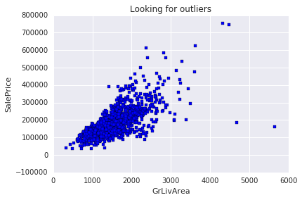
# Log transform the target for official scoring
train.SalePrice = np.log1p(train.SalePrice)
y = train.SalePrice
显而易见这是log变换。
3.按业务含义填充缺失值
# 特殊处理【无法用平均值/众数填充】的特征缺失值
# 规则:严格按照数据集官方说明,NA 代表特定含义(不是真的缺失)

# Alley(小巷通道):NA = 没有小巷通道 → 填 None
train.loc[:, "Alley"] = train.loc[:, "Alley"].fillna("None")

# BedroomAbvGr(地上卧室数):NA 大概率 = 0 → 填 0
train.loc[:, "BedroomAbvGr"] = train.loc[:, "BedroomAbvGr"].fillna(0)

# 地下室相关特征:NA = 没有地下室 → 统一填 No / 0
train.loc[:, "BsmtQual"] = train.loc[:, "BsmtQual"].fillna("No")
train.loc[:, "BsmtCond"] = train.loc[:, "BsmtCond"].fillna("No")
train.loc[:, "BsmtExposure"] = train.loc[:, "BsmtExposure"].fillna("No")
train.loc[:, "BsmtFinType1"] = train.loc[:, "BsmtFinType1"].fillna("No")
train.loc[:, "BsmtFinType2"] = train.loc[:, "BsmtFinType2"].fillna("No")
train.loc[:, "BsmtFullBath"] = train.loc[:, "BsmtFullBath"].fillna(0)
train.loc[:, "BsmtHalfBath"] = train.loc[:, "BsmtHalfBath"].fillna(0)
train.loc[:, "BsmtUnfSF"] = train.loc[:, "BsmtUnfSF"].fillna(0)

# CentralAir(中央空调):NA = 没有 → 填 N
train.loc[:, "CentralAir"] = train.loc[:, "CentralAir"].fillna("N")

# 环境条件:NA = 正常 → 填 Norm
train.loc[:, "Condition1"] = train.loc[:, "Condition1"].fill("Norm")
train.loc[:, "Condition2"] = train.loc[:, "Condition2"].fill("Norm")

# 封闭门廊:NA = 没有 → 填 0
train.loc[:, "EnclosedPorch"] = train.loc[:, "EnclosedPorch"].fillna(0)

# 外墙质量/条件:NA = 一般水平 → 填 TA(Typical/Average)
train.loc[:, "ExterCond"] = train.loc[:, "ExterCond"].fillna("TA")
train.loc[:, "ExterQual"] = train.loc[:, "ExterQual"].fillna("TA")

# Fence(围栏):NA = 没有围栏 → 填 No
train.loc[:, "Fence"] = train.loc[:, "Fence"].fillna("No")

# 壁炉相关:NA = 没有壁炉 → 填 No / 0
train.loc[:, "FireplaceQu"] = train.loc[:, "FireplaceQu"].fillna("No")
train.loc[:, "Fireplaces"] = train.loc[:, "Fireplaces"].fillna(0)

# Functional(功能评级):NA = 典型正常 → 填 Typ
train.loc[:, "Functional"] = train.loc[:, "Functional"].fillna("Typ")

# 车库相关特征:NA = 没有车库 → 填 No / 0
train.loc[:, "GarageType"] = train.loc[:, "GarageType"].fillna("No")
train.loc[:, "GarageFinish"] = train.loc[:, "GarageFinish"].fillna("No")
train.loc[:, "GarageQual"] = train.loc[:, "GarageQual"].fillna("No")
train.loc[:, "GarageCond"] = train.loc[:, "GarageCond"].fillana("No")
train.loc[:, "GarageArea"] = train.loc[:, "GarageArea"].fillna(0)
train.loc[:, "GarageCars"] = train.loc[:, "GarageCars"].fillna(0)

# 半浴室:NA = 0 → 填 0
train.loc[:, "HalfBath"] = train.loc[:, "HalfBath"].fillna(0)

# 供暖质量:NA = 一般 → 填 TA
train.loc[:, "HeatingQC"] = train.loc[:, "HeatingQC"].fillna("TA")

# 厨房数量/质量:NA = 0 / 一般 → 填 0 / TA
train.loc[:, "KitchenAbvGr"] = train.loc[:, "KitchenAbvGr"].fillna(0)
train.loc[:, "KitchenQual"] = train.loc[:, "KitchenQual"].fillna("TA")

# 临街距离:NA = 没有临街 → 填 0
train.loc[:, "LotFrontage"] = train.loc[:, "LotFrontage"].fillna(0)

# 地块形状:NA = 规则 → 填 Reg
train.loc[:, "LotShape"] = train.loc[:, "LotShape"].fillna("Reg")

# 砖石饰面:NA = 没有 → 填 None / 0
train.loc[:, "MasVnrType"] = train.loc[:, "MasVnrType"].fillna("None")
train.loc[:, "MasVnrArea"] = train.loc[:, "MasVnrArea"].fillna(0)

# 额外设施:NA = 没有 → 填 No / 0
train.loc[:, "MiscFeature"] = train.loc[:, "MiscFeature"].fillna("No")
train.loc[:, "MiscVal"] = train.loc[:, "MiscVal"].fillna(0)

# 开放式门廊:NA = 没有 → 填 0
train.loc[:, "OpenPorchSF"] = train.loc[:, "OpenPorchSF"].fillna(0)

# 铺装车道:NA = 未铺装 → 填 N
train.loc[:, "PavedDrive"] = train.loc[:, "PavedDrive"].fillna("N")

# 泳池相关:NA = 没有泳池 → 填 No / 0
train.loc[:, "PoolQC"] = train.loc[:, "PoolQC"].fillna("No")
train.loc[:, "PoolArea"] = train.loc[:, "PoolArea"].fillna(0)

# 销售条件:NA = 正常销售 → 填 Normal
train.loc[:, "SaleCondition"] = train.loc[:, "SaleCondition"].fillna("Normal")

# 屏风门廊:NA = 没有 → 填 0
train.loc[:, "ScreenPorch"] = train.loc[:, "ScreenPorch"].fillna(0)

# 总房间数:NA = 0 → 填 0
train.loc[:, "TotRmsAbvGrd"] = train.loc[:, "TotRmsAbvGrd"].fillna(0)

# 公共设施:NA = 全套市政设施 → 填 AllPub
train.loc[:, "Utilities"] = train.loc[:, "Utilities"].fillna("AllPub")

# 木质露台:NA = 没有 → 填 0
train.loc[:, "WoodDeckSF"] = train.loc[:, "WoodDeckSF"].fillna(0)
这是一种值得学习的新处理方法,不再使用粗暴填充,而是按照NA的实际意义填充,NA 大部分代表 “没有这个设施” → 填 No / 0。
4.假数值特征转换为分类特征
# 【重点】有些数值型特征,本质上是【分类特征】
# 必须把数字转成文字类别,模型才能正确理解
train = train.replace({
    # 1. 房屋子类 MSSubClass(数字代表房屋类型)
    "MSSubClass" : {
        20 : "SC20", 30 : "SC30", 40 : "SC40", 45 : "SC45",
        50 : "SC50", 60 : "SC60", 70 : "SC70", 75 : "SC75",
        80 : "SC80", 85 : "SC85", 90 : "SC90", 120 : "SC120",
        150 : "SC150", 160 : "SC160", 180 : "SC180", 190 : "SC190"
    },
    # 2. 销售月份 MoSold(数字1-12代表1-12月)
    "MoSold" : {
        1 : "Jan", 2 : "Feb", 3 : "Mar", 4 : "Apr",
        5 : "May", 6 : "Jun", 7 : "Jul", 8 : "Aug",
        9 : "Sep", 10 : "Oct", 11 : "Nov", 12 : "Dec"
    }
})
为什么要这么做?
- MSSubClass:虽然是数字(20,30,60...),但代表房屋类型
- 20 ≠ 2×10,它只是一个代号
- MoSold:数字 1-12 代表月份
- 1 月 ≠ 1,12 月 ≠ 12,没有大小关系
防止模型把分类代号当成数字计算,大幅提升预测准确率。
5.有序分类特征进行有序编码
# 把【有等级、有好坏顺序】的分类文字,编码成【有序数字】
# 例如:差(Po)=1,一般(TA)=3,优秀(Ex)=5
train = train.replace({

    # 小巷类型:泥土=1,铺砖=2 (铺砖更好)
    "Alley" : {"Grvl" : 1, "Pave" : 2},

    # 地下室条件:无=0 → 差=1 → 优秀=5
    "BsmtCond" : {"No" : 0, "Po" : 1, "Fa" : 2, "TA" : 3, "Gd" : 4, "Ex" : 5},

    # 下面所有特征都是同理:
    # 质量/条件/类型 → 按好坏排序 → 转成 0,1,2,3,4,5...
    "BsmtExposure" : {"No" : 0, "Mn" : 1, "Av": 2, "Gd" : 3},
    "BsmtFinType1" : {"No" : 0, "Unf" : 1, "LwQ": 2, "Rec" : 3, "BLQ" : 4, "ALQ" : 5, "GLQ" : 6},
    "BsmtFinType2" : {"No" : 0, "Unf" : 1, "LwQ": 2, "Rec" : 3, "BLQ" : 4, "ALQ" : 5, "GLQ" : 6},
    "BsmtQual" : {"No" : 0, "Po" : 1, "Fa" : 2, "TA": 3, "Gd" : 4, "Ex" : 5},
    "ExterCond" : {"Po" : 1, "Fa" : 2, "TA": 3, "Gd": 4, "Ex" : 5},
    "ExterQual" : {"Po" : 1, "Fa" : 2, "TA": 3, "Gd": 4, "Ex" : 5},
    "FireplaceQu" : {"No" : 0, "Po" : 1, "Fa" : 2, "TA" : 3, "Gd" : 4, "Ex" : 5},
    "Functional" : {"Sal" : 1, "Sev" : 2, "Maj2" : 3, "Maj1" : 4, "Mod": 5, "Min2" : 6, "Min1" : 7, "Typ" : 8},
    "GarageCond" : {"No" : 0, "Po" : 1, "Fa" : 2, "TA" : 3, "Gd" : 4, "Ex" : 5},
    "GarageQual" : {"No" : 0, "Po" : 1, "Fa" : 2, "TA" : 3, "Gd" : 4, "Ex" : 5},
    "HeatingQC" : {"Po" : 1, "Fa" : 2, "TA" : 3, "Gd" : 4, "Ex" : 5},
    "KitchenQual" : {"Po" : 1, "Fa" : 2, "TA" : 3, "Gd" : 4, "Ex" : 5},
    "LandSlope" : {"Sev" : 1, "Mod" : 2, "Gtl" : 3},
    "LotShape" : {"IR3" : 1, "IR2" : 2, "IR1" : 3, "Reg" : 4},
    "PavedDrive" : {"N" : 0, "P" : 1, "Y" : 2},
    "PoolQC" : {"No" : 0, "Fa" : 1, "TA" : 2, "Gd" : 3, "Ex" : 4},
    "Street" : {"Grvl" : 1, "Pave" : 2},
    "Utilities" : {"ELO" : 1, "NoSeWa" : 2, "NoSewr" : 3, "AllPub" : 4}
})- 这是 有序编码(Ordinal Encoding)
- 专门处理:有好坏、等级、顺序的特征
- 目的:让模型看懂 “质量越好,价值越高”
- 线性回归必须做这一步,否则模型看不懂文字
相对于独热编码,有序编码优势:
- 保留等级信息(模型更准)
- 不增加特征列(不爆炸维度)
- 速度快、过拟合风险低
- 完美适配线性回归
6.高阶特征工程
接下来,我们将通过3 种方式构造新特征:
- 对现有特征进行简化
- 组合现有特征生成新特征
- 对最重要的 10 个特征做多项式变换
简化现有特征
# ====================== 创造新特征 ======================
# 1. 简化现有特征(把复杂等级 → 简单大分类)

# 整体品质 (1-10分) → 简化为 3档:差(1)、平均(2)、好(3)
train["SimplOverallQual"] = train.OverallQual.replace({
    1 : 1, 2 : 1, 3 : 1,   # 差
    4 : 2, 5 : 2, 6 : 2,   # 平均
    7 : 3, 8 : 3, 9 : 3, 10 : 3 # 好
})

# 整体条件 → 同样简化为 3档
train["SimplOverallCond"] = train.OverallCond.replace({
    1 : 1, 2 : 1, 3 : 1,
    4 : 2, 5 : 2, 6 : 2,
    7 : 3, 8 : 3, 9 : 3, 10 : 3
})

# 泳池质量 → 简化为 2档:平均、好
train["SimplPoolQC"] = train.PoolQC.replace({
    1 : 1, 2 : 1,
    3 : 2, 4 : 2
})

# 车库条件 → 简化为 2档:差/平均、好
train["SimplGarageCond"] = train.GarageCond.replace({
    1 : 1,
    2 : 1, 3 : 1,
    4 : 2, 5 : 2
})

# 车库质量 → 同上简化
train["SimplGarageQual"] = train.GarageQual.replace({
    1 : 1,
    2 : 1, 3 : 1,
    4 : 2, 5 : 2
})

# 壁炉质量 → 简化
train["SimplFireplaceQu"] = train.FireplaceQu.replace({
    1 : 1,
    2 : 1, 3 : 1,
    4 : 2, 5 : 2
})

# 房屋功能 → 按损坏程度简化为4档
train["SimplFunctional"] = train.Functional.replace({
    1 : 1, 2 : 1,         # 严重损坏
    3 : 2, 4 : 2,         # 主要损坏
    5 : 3, 6 : 3, 7 : 3,  # 轻微损坏
    8 : 4                 # 正常
})

# 厨房质量、供暖质量、地下室各类质量...
# 全部都是:把细分等级 → 合并成简单大类
# 规则一模一样:差→1,平均→2,好→3
train["SimplKitchenQual"] = train.KitchenQual.replace({...})
train["SimplHeatingQC"] = train.HeatingQC.replace({...})
train["SimplBsmtFinType1"] = train.BsmtFinType1.replace({...})
train["SimplBsmtFinType2"] = train.BsmtFinType2.replace({...})
train["SimplBsmtCond"] = train.BsmtCond.replace({...})
train["SimplBsmtQual"] = train.BsmtQual.replace({...})
train["SimplExterCond"] = train.ExterCond.replace({...})
train["SimplExterQual"] = train.ExterQual.replace({...})- 把 10 个等级 → 3 个大类
- 让模型只抓大规律:差、中、好
- 更稳定、泛化能力更强
组合现有特征
# ====================== 2. 组合现有特征 ======================
# 核心思路:数量 × 质量 = 综合评分;同类面积相加 = 总面积

# 房屋综合等级 = 整体品质 × 整体条件
train["OverallGrade"] = train["OverallQual"] * train["OverallCond"]

# 车库综合等级 = 车库质量 × 车库条件
train["GarageGrade"] = train["GarageQual"] * train["GarageCond"]

# 外墙综合等级 = 外墙质量 × 外墙条件
train["ExterGrade"] = train["ExterQual"] * train["ExterCond"]

# 厨房综合评分 = 厨房数量 × 厨房质量
train["KitchenScore"] = train["KitchenAbvGr"] * train["KitchenQual"]

# 壁炉综合评分 = 壁炉数量 × 壁炉质量
train["FireplaceScore"] = train["Fireplaces"] * train["FireplaceQu"]

# 车库综合评分 = 车库面积 × 车库质量
train["GarageScore"] = train["GarageArea"] * train["GarageQual"]

# 泳池综合评分 = 泳池面积 × 泳池质量
train["PoolScore"] = train["PoolArea"] * train["PoolQC"]

# ----- 简化版特征组合(和上面逻辑一样,只是用了简化后的质量)-----
train["SimplOverallGrade"] = train["SimplOverallQual"] * train["SimplOverallCond"]
train["SimplExterGrade"] = train["SimplExterQual"] * train["SimplExterCond"]
train["SimplPoolScore"] = train["PoolArea"] * train["SimplPoolQC"]
train["SimplGarageScore"] = train["GarageArea"] * train["SimplGarageQual"]
train["SimplFireplaceScore"] = train["Fireplaces"] * train["SimplFireplaceQu"]
train["SimplKitchenScore"] = train["KitchenAbvGr"] * train["SimplKitchenQual"]

# 【关键】总浴室数 = 地下室全浴 + 0.5*地下室半浴 + 地上全浴 + 0.5*地上半浴
train["TotalBath"] = train["BsmtFullBath"] + (0.5 * train["BsmtHalfBath"]) + train["FullBath"] + (0.5 * train["HalfBath"])

# 房屋总面积(含地下室)= 地上居住面积 + 地下室总面积
train["AllSF"] = train["GrLivArea"] + train["TotalBsmtSF"]

# 一二楼总面积 = 1楼面积 + 2楼面积
train["AllFlrsSF"] = train["1stFlrSF"] + train["2ndFlrSF"]

# 门廊总面积 = 所有类型门廊面积相加
train["AllPorchSF"] = train["OpenPorchSF"] + train["EnclosedPorch"] + train["3SsnPorch"] + train["ScreenPorch"]

# 是否有砖石饰面 = 有则为1,无为0
train["HasMasVnr"] = train.MasVnrType.replace({"BrkCmn" : 1, "BrkFace" : 1, "CBlock" : 1, "Stone" : 1, "None" : 0})

# 是否按规划购买(新房)= Partial是1,其他是0
train["BoughtOffPlan"] = train.SaleCondition.replace({"Abnorml" : 0, "Alloca" : 0, "AdjLand" : 0, "Family" : 0, "Normal" : 0, "Partial" : 1})
最经典的两个组合特征:
TotalBath(总浴室数)半浴室算 0.5,全浴室算 1,全部加起来。AllSF(总面积)地上面积 + 地下室面积。
对重要特征做多项式变换
# 找出与目标值(房价 SalePrice)相关性最强的特征
print("Find most important features relative to target")

# 1. 计算所有特征之间的【相关系数矩阵】
# corr 值越接近 1 → 正相关越强(特征越大,房价越高)
# corr 值越接近 -1 → 负相关越强
corr = train.corr()

# 2. 按照 "SalePrice"(房价)这一列排序
# ascending = False → 从大到小降序排列(最强的放最上面)
# inplace = True → 直接修改原数据,不用赋值
corr.sort_values(["SalePrice"], ascending = False, inplace = True)

# 3. 只打印出【每个特征与房价的相关性大小】
print(corr.SalePrice)
out:
Find most important features relative to target
SalePrice 1.000
OverallQual 0.819
AllSF 0.817
AllFlrsSF 0.729
GrLivArea 0.719
SimplOverallQual 0.708
ExterQual 0.681
GarageCars 0.680
TotalBath 0.673
KitchenQual 0.667
GarageScore 0.657
GarageArea 0.655
TotalBsmtSF 0.642
SimplExterQual 0.636
SimplGarageScore 0.631
BsmtQual 0.615
1stFlrSF 0.614
SimplKitchenQual 0.610
OverallGrade 0.604
SimplBsmtQual 0.594
FullBath 0.591
YearBuilt 0.589
ExterGrade 0.587
YearRemodAdd 0.569
FireplaceQu 0.547
GarageYrBlt 0.544
TotRmsAbvGrd 0.533
SimplOverallGrade 0.527
SimplKitchenScore 0.523
FireplaceScore 0.518
...
SimplBsmtCond 0.204
BedroomAbvGr 0.204
AllPorchSF 0.199
LotFrontage 0.174
SimplFunctional 0.137
Functional 0.136
ScreenPorch 0.124
SimplBsmtFinType2 0.105
Street 0.058
3SsnPorch 0.056
ExterCond 0.051
PoolArea 0.041
SimplPoolScore 0.040
SimplPoolQC 0.040
PoolScore 0.040
PoolQC 0.038
BsmtFinType2 0.016
Utilities 0.013
BsmtFinSF2 0.006
BsmtHalfBath -0.015
MiscVal -0.020
SimplOverallCond -0.028
YrSold -0.034
OverallCond -0.037
LowQualFinSF -0.038
LandSlope -0.040
SimplExterCond -0.042
KitchenAbvGr -0.148
EnclosedPorch -0.149
LotShape -0.286
Name: SalePrice, dtype: float64
# 第三种:对相关性最高的 Top10 特征 做多项式变换
# 每个重要特征都生成 3 个新特征:平方、立方、平方根

# 1. 整体品质 OverallQual
train["OverallQual-s2"] = train["OverallQual"] ** 2   # 平方
train["OverallQual-s3"] = train["OverallQual"] ** 3   # 立方
train["OverallQual-Sq"] = np.sqrt(train["OverallQual"]) # 平方根

# 2. 总面积 AllSF
train["AllSF-2"] = train["AllSF"] ** 2
train["AllSF-3"] = train["AllSF"] ** 3
train["AllSF-Sq"] = np.sqrt(train["AllSF"])

# 3. 总楼层面积 AllFlrsSF
train["AllFlrsSF-2"] = train["AllFlrsSF"] ** 2
train["AllFlrsSF-3"] = train["AllFlrsSF"] ** 3
train["AllFlrsSF-Sq"] = np.sqrt(train["AllFlrsSF"])

# 4. 地上居住面积 GrLivArea
train["GrLivArea-2"] = train["GrLivArea"] ** 2
train["GrLivArea-3"] = train["GrLivArea"] ** 3
train["GrLivArea-Sq"] = np.sqrt(train["GrLivArea"])

# 后面所有特征逻辑完全一样:
# 每个强特征 → 做 平方、立方、根号
train["SimplOverallQual-s2"] = train["SimplOverallQual"] ** 2
train["SimplOverallQual-s3"] = train["SimplOverallQual"] ** 3
train["SimplOverallQual-Sq"] = np.sqrt(train["SimplOverallQual"])

train["ExterQual-2"] = train["ExterQual"] ** 2
train["ExterQual-3"] = train["ExterQual"] ** 3
train["ExterQual-Sq"] = np.sqrt(train["ExterQual"])

train["GarageCars-2"] = train["GarageCars"] ** 2
train["GarageCars-3"] = train["GarageCars"] ** 3
train["GarageCars-Sq"] = np.sqrt(train["GarageCars"])

train["TotalBath-2"] = train["TotalBath"] ** 2
train["TotalBath-3"] = train["TotalBath"] ** 3
train["TotalBath-Sq"] = np.sqrt(train["TotalBath"])

train["KitchenQual-2"] = train["KitchenQual"] ** 2
train["KitchenQual-3"] = train["KitchenQual"] ** 3
train["KitchenQual-Sq"] = np.sqrt(train["KitchenQual"])

train["GarageScore-2"] = train["GarageScore"] ** 2
train["GarageScore-3"] = train["GarageScore"] ** 3
train["GarageScore-Sq"] = np.sqrt(train["GarageScore"])
为什么要做多项式?
1. 线性回归的天生缺陷
普通线性回归只能画直线:房价 = a×面积 + b
但真实房价和面积不是直线关系,而是曲线:
- 面积小 → 涨价慢
- 面积大 → 涨价飞快
2. 多项式 = 把直线变曲线
加了平方 / 立方后,模型就能学习弯曲的规律:房价 = a×面积 + b×面积² + c×面积³
为什么只对 Top10 特征做?
- 只有和房价高度相关的特征才值得加工
- 无关特征做多项式只会增加噪声、过拟合
- 这是高效提分的关键
三种变换分别什么意思?
**2平方放大数值大的特征(抓暴涨趋势)**3立方进一步放大非线性(让曲线更弯)np.sqrt()平方根压缩极端值(让数据更平滑)
这里有一个思考,这种变换这么麻烦,为什么不用激活函数呢?
- 激活函数 = 神经网络的非线性
- 多项式特征 = 线性回归的非线性
那我如果改用mlp,多项式变换是不是就可以不用做了,或者说做了也效果不大?
是的,不用加
如果给 MLP 也加上多项式,会出现 3 个坏处:
- 特征冗余MLP 自己已经学到 x² 了,你再给它 x² → 重复信息
- 维度爆炸特征变多,计算更慢,更容易过拟合
- 效果几乎不变,甚至下降手工构造永远比不上神经网络自动学习
那 MLP 应该用什么特征?
只用原始特征就够了!
- 面积
- 质量评分
- 房间数
- 浴室数
- 各种类别特征(做独热编码就行)
MLP 会自动学习:
- 非线性关系
- 特征交互
- 高阶多项式
- 隐藏规律
7.特征常规处理
# 区分:数值型特征 和 类别型特征(排除目标值 SalePrice)
# 1. 选出所有【文本/类别类型】的列(object = 文字类型)
categorical_features = train.select_dtypes(include = ["object"]).columns

# 2. 选出所有【非object】的列 = 数值型列(int/float)
numerical_features = train.select_dtypes(exclude = ["object"]).columns

# 3. 数值特征里**删掉房价 SalePrice**
# 因为 SalePrice 是目标值y,不是特征X
numerical_features = numerical_features.drop("SalePrice")

# 打印数量,方便确认
print("Numerical features : " + str(len(numerical_features)))
print("Categorical features : " + str(len(categorical_features)))

# 分开存储:
train_num = train[numerical_features]    # 数值特征
train_cat = train[categorical_features] # 类别特征
Numerical features : 117 Categorical features : 26
# 用【中位数】填充数值特征中**剩余的**缺失值
# 1. 先统计数值特征里还有多少个缺失值(NA)
print("NAs for numerical features in train : " + str(train_num.isnull().values.sum()))

# 2. 用每一列的中位数填充该列的缺失值
train_num = train_num.fillna(train_num.median())

# 3. 再次检查,确认缺失值已经变成 0 个
print("Remaining NAs for numerical features in train : " + str(train_num.isnull().values.sum()))
NAs for numerical features in train : 81 Remaining NAs for numerical features in train : 0
这里是对真正缺失的缺失值进行中位数填充
# 对【偏斜的数值特征】做对数变换,减少异常值的极端影响
# 经验规则:偏度绝对值 > 0.5,就算中度偏斜
skewness = train_num.apply(lambda x: skew(x))  # 计算每个数值特征的偏度
skewness = skewness[abs(skewness) > 0.5]        # 筛选出偏度大的特征
print(str(skewness.shape[0]) + " skewed numerical features to log transform")

skewed_features = skewness.index               # 取出要处理的特征名
train_num[skewed_features] = np.log1p(train_num[skewed_features])  # 对数变换
86 skewed numerical features to log transform
对数值型特征根据偏度进行log变换
# 对类别特征进行 独热编码(One-Hot Encoding)
# 1. 先检查类别特征有没有缺失值(理论上应该是0)
print("NAs for categorical features in train : " + str(train_cat.isnull().values.sum()))

# 2. 一键独热编码:文字类别 → 0/1数字列
train_cat = pd.get_dummies(train_cat)

# 3. 再次确认:编码后也没有缺失值
print("Remaining NAs for categorical features in train : " + str(train_cat.isnull().values.sum()))
NAs for categorical features in train : 1 Remaining NAs for categorical features in train : 0
对类别特征进行独热编码
8.数据集划分
# 把 数值特征 + 类别特征 拼接在一起
train = pd.concat([train_num, train_cat], axis = 1)
print("New number of features : " + str(train.shape[1]))

# 把数据集分成:训练集 + 验证集
X_train, X_test, y_train, y_test = train_test_split(train, y, test_size = 0.3, random_state = 0)

# 打印形状,确认数据没问题
print("X_train : " + str(X_train.shape))
print("X_test : " + str(X_test.shape))
print("y_train : " + str(y_train.shape))
print("y_test : " + str(y_test.shape))
New number of features : 319 X_train : (1019, 319) X_test : (437, 319) y_train : (1019,) y_test : (437,)
9.数据标准化
# 对数值特征进行标准化(缩放成均值0,标准差1)
stdSc = StandardScaler()

# 1. 在训练集上「学习」均值和标准差,然后直接标准化
X_train.loc[:, numerical_features] = stdSc.fit_transform(X_train.loc[:, numerical_features])

# 2. 用训练集学到的均值&标准差,标准化测试集(绝对不能重新学习!)
X_test.loc[:, numerical_features] = stdSc.transform(X_test.loc[:, numerical_features])
标准化不能在数据集划分之前做,因为我们不想让 StandardScaler 在后续会被用作测试集的样本上进行拟合。
Q1:这里我对数据泄露和标准化处理流程产生了疑问(后文中会进行总结)
10.定义RMSE损失函数
# 定义官方评估指标:RMSE
scorer = make_scorer(mean_squared_error, greater_is_better = False)

# 定义函数:计算训练集的 10折交叉验证 RMSE
def rmse_cv_train(model):
    rmse= np.sqrt(-cross_val_score(model, X_train, y_train, scoring = scorer, cv = 10))
    return(rmse)

# 定义函数:计算测试集的 10折交叉验证 RMSE
def rmse_cv_test(model):
    rmse= np.sqrt(-cross_val_score(model, X_test, y_test, scoring = scorer, cv = 10))
    return(rmse)
原文:我的本地交叉验证结果与公共排行榜上的数值相差很大,所以我有点担心我的交叉验证流程可能在某个地方存在问题。如果你发现了问题,请告诉我。
因为测试集不需要做交叉验证。
1. 交叉验证 = 反复考试
CV 会把数据切 10 次,训练 10 次,测 10 次。测试集如果被 CV 用了 = 考题泄露 10 次!
2. 测试集的使命:只在模型完全训练好后,评测一次
用测试集做 CV =模型提前偷看答案 → 本地分数造假 → 上线崩盘
11.线性回归模型
# 训练线性回归模型
lr = LinearRegression()
lr.fit(X_train, y_train)
# 输出训练集和测试集上的交叉验证RMSE(评估模型误差)
print("RMSE on Training set :", rmse_cv_train(lr).mean())
print("RMSE on Test set :", rmse_cv_test(lr).mean())
# 用训练好的模型分别对训练集、测试集做预测
y_train_pred = lr.predict(X_train)
y_test_pred = lr.predict(X_test)
# 绘制残差图:横坐标为预测值,纵坐标为残差(预测值-真实值)
# 蓝色=训练集,绿色=测试集,红线为0残差线
# 用于观察残差是否随机分布,判断模型拟合是否合理
plt.scatter(y_train_pred, y_train_pred - y_train, c = "blue", marker = "s", label = "Training data")
plt.scatter(y_test_pred, y_test_pred - y_test, c = "lightgreen", marker = "s", label = "Validation data")
plt.title("Linear regression")
plt.xlabel("Predicted values")
plt.ylabel("Residuals")
plt.legend(loc = "upper left")
plt.hlines(y = 0, xmin = 10.5, xmax = 13.5, color = "red")
plt.show()
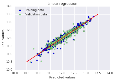
# 绘制预测值vs真实值图:横坐标预测值,纵坐标真实值
# 红色直线代表完美预测(预测值=真实值),点越靠近红线说明预测越准确
plt.scatter(y_train_pred, y_train, c = "blue", marker = "s", label = "Training data")
plt.scatter(y_test_pred, y_test, c = "lightgreen", marker = "s", label = "Validation data")
plt.title("Linear regression")
plt.xlabel("Predicted values")
plt.ylabel("Real values")
plt.legend(loc = "upper left")
plt.plot([10.5, 13.5], [10.5, 13.5], c = "red")
plt.show()RMSE on Training set : 15758371373.7 RMSE on Test set : 0.395779797728
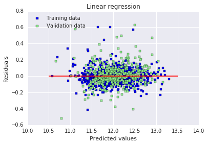
原文:出于某种原因,这里训练集上的 RMSE 显示得很奇怪(在我自己电脑上运行时则不会)。误差似乎是随机分布的,并且在中心线附近随机分散,至少情况是这样的。这意味着我们的模型能够捕捉到大部分的解释性信息。
12.L2正则化
# 2* Ridge
# 初始化RidgeCV模型,传入一组alpha值,自动交叉验证选择最优正则化系数
ridge = RidgeCV(alphas = [0.01, 0.03, 0.06, 0.1, 0.3, 0.6, 1, 3, 6, 10, 30, 60])
# 在训练集上训练模型,自动筛选最优alpha
ridge.fit(X_train, y_train)
# 获取模型选出的最优alpha值
alpha = ridge.alpha_
# 打印最优alpha
print("Best alpha :", alpha)
# 在第一轮最优alpha的基础上,缩小范围再次搜索更精确的alpha值
print("Try again for more precision with alphas centered around " + str(alpha))
ridge = RidgeCV(alphas = [alpha * .6, alpha * .65, alpha * .7, alpha * .75, alpha * .8, alpha * .85,
alpha * .9, alpha * .95, alpha, alpha * 1.05, alpha * 1.1, alpha * 1.15,
alpha * 1.25, alpha * 1.3, alpha * 1.35, alpha * 1.4],
cv = 10) # 设置10折交叉验证
ridge.fit(X_train, y_train)
alpha = ridge.alpha_
print("Best alpha :", alpha)
# 计算并输出岭回归在训练集、测试集上的RMSE
print("Ridge RMSE on Training set :", rmse_cv_train(ridge).mean())
print("Ridge RMSE on Test set :", rmse_cv_test(ridge).mean())
# 对训练集和测试集进行预测
y_train_rdg = ridge.predict(X_train)
y_test_rdg = ridge.predict(X_test)
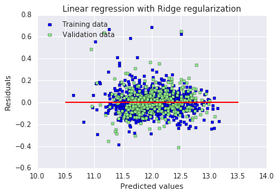
# 绘制残差图:横坐标为预测值,纵坐标为残差(预测值-真实值)
# 蓝色点代表训练集,绿色点代表验证集,红色线为0残差参考线
plt.scatter(y_train_rdg, y_train_rdg - y_train, c = "blue", marker = "s", label = "Training data")
plt.scatter(y_test_rdg, y_test_rdg - y_test, c = "lightgreen", marker = "s", label = "Validation data")
plt.title("Linear regression with Ridge regularization")
plt.xlabel("Predicted values")
plt.ylabel("Residuals")
plt.legend(loc = "upper left")
plt.hlines(y = 0, xmin = 10.5, xmax = 13.5, color = "red")
plt.show()
# 绘制预测值与真实值对比图
# 红色直线代表完美预测(预测值=真实值),点越贴近红线表示预测效果越好
plt.scatter(y_train_rdg, y_train, c = "blue", marker = "s", label = "Training data")
plt.scatter(y_test_rdg, y_test, c = "lightgreen", marker = "s", label = "Validation data")
plt.title("Linear regression with Ridge regularization")
plt.xlabel("Predicted values")
plt.ylabel("Real values")
plt.legend(loc = "upper left")
plt.plot([10.5, 13.5], [10.5, 13.5], c = "red")
plt.show()
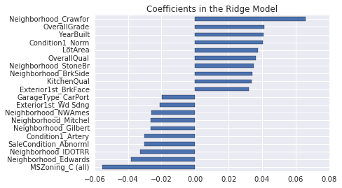
# 分析并可视化模型的特征系数
coefs = pd.Series(ridge.coef_, index = X_train.columns)
# 统计模型使用的特征数(系数非0)和被剔除的特征数(系数为0)
print("Ridge picked " + str(sum(coefs != 0)) + " features and eliminated the other " + \
str(sum(coefs == 0)) + " features")
# 提取系数最小的10个和最大的10个特征
imp_coefs = pd.concat([coefs.sort_values().head(10), coefs.sort_values().tail(10)])
# 水平条形图展示重要特征的系数
imp_coefs.plot(kind = "barh")
plt.title("Coefficients in the Ridge Model")
plt.show()Best alpha : 30.0 Try again for more precision with alphas centered around 30.0 Best alpha : 24.0 Ridge RMSE on Training set : 0.115405723285 Ridge RMSE on Test set : 0.116427213778

Ridge picked 316 features and eliminated the other 3 features
严格来说:
Lasso(L1)会真正把系数压到 0 → 真正删除特征
Ridge(L2)几乎不会把系数压到 0 → 不会真正删除特征
为什么 Ridge 也会出现系数 = 0?
原因只有 3 个,都是正常情况:
- 那些特征本来就是常数(所有值都一样)模型学不到东西,系数自然变成 0
- 那些特征完全和其他特征重复(多重共线性)冗余特征,系数被压成 0
- 数值计算的微小精度问题极小系数被系统当成 0
原文:加入正则化之后,我们现在得到了效果好得多的 RMSE。训练集和测试集结果之间的微小差异表明,我们已经消除了大部分过拟合。从图表上看,也直观地证实了这一点。
13.L1正则化
# 3* Lasso
# 第一次粗搜最优alpha,LassoCV自动交叉验证选最佳惩罚系数
lasso = LassoCV(alphas = [0.0001, 0.0003, 0.0006, 0.001, 0.003, 0.006, 0.01, 0.03, 0.06, 0.1,
                          0.3, 0.6, 1],
                max_iter = 50000, cv = 10)
lasso.fit(X_train, y_train)
alpha = lasso.alpha_
print("Best alpha :", alpha)

# 在最优alpha附近细搜,得到更精确的正则化强度
print("Try again for more precision with alphas centered around " + str(alpha))
lasso = LassoCV(alphas = [alpha * .6, alpha * .65, alpha * .7, alpha * .75, alpha * .8,
                          alpha * .85, alpha * .9, alpha * .95, alpha, alpha * 1.05,
                          alpha * 1.1, alpha * 1.15, alpha * 1.25, alpha * 1.3, alpha * 1.35,
                          alpha * 1.4],
                max_iter = 50000, cv = 10)
lasso.fit(X_train, y_train)
alpha = lasso.alpha_
print("Best alpha :", alpha)

# 输出训练集与测试集的10折交叉验证RMSE
print("Lasso RMSE on Training set :", rmse_cv_train(lasso).mean())
print("Lasso RMSE on Test set :", rmse_cv_test(lasso).mean())

# 模型预测
y_train_las = lasso.predict(X_train)
y_test_las = lasso.predict(X_test)

# 绘制残差图:看误差是否随机分布
plt.scatter(y_train_las, y_train_las - y_train, c = "blue", marker = "s", label = "Training data")
plt.scatter(y_test_las, y_test_las - y_test, c = "lightgreen", marker = "s", label = "Validation data")
plt.title("Linear regression with Lasso regularization")
plt.xlabel("Predicted values")
plt.ylabel("Residuals")
plt.legend(loc = "upper left")
plt.hlines(y = 0, xmin = 10.5, xmax = 13.5, color = "red")
plt.show()

# 绘制预测值 vs 真实值图:越靠近红线越准
plt.scatter(y_train_las, y_train, c = "blue", marker = "s", label = "Training data")
plt.scatter(y_test_las, y_test, c = "lightgreen", marker = "s", label = "Validation data")
plt.title("Linear regression with Lasso regularization")
plt.xlabel("Predicted values")
plt.ylabel("Real values")
plt.legend(loc = "upper left")
plt.plot([10.5, 13.5], [10.5, 13.5], c = "red")
plt.show()

# 输出Lasso选择了多少特征、删除了多少特征
# Lasso会把大量系数变成0,实现自动特征选择
coefs = pd.Series(lasso.coef_, index = X_train.columns)
print("Lasso picked " + str(sum(coefs != 0)) + " features and eliminated the other " +  \
      str(sum(coefs == 0)) + " features")

# 画出系数最大/最小的10个重要特征
imp_coefs = pd.concat([coefs.sort_values().head(10),
                     coefs.sort_values().tail(10)])
imp_coefs.plot(kind = "barh")
plt.title("Coefficients in the Lasso Model")
plt.show()
Best alpha : 0.0006 Try again for more precision with alphas centered around 0.0006 Best alpha : 0.0006 Lasso RMSE on Training set : 0.114111508375 Lasso RMSE on Test set : 0.115832132218

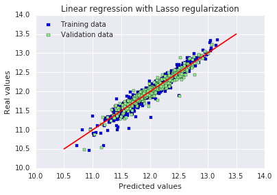
Lasso picked 110 features and eliminated the other 209 features

原文:训练集和测试集上的 RMSE 结果都变得更好了。最有趣的是,Lasso 只使用了三分之一的可用特征。另一个有趣的细节是:它似乎给了不同街区类别很大的权重,包括正向和负向的权重。从直观上看这是合理的,在同一座城市里,不同街区的房价差异非常大。
与其他特征相比,“MSZoning_C (all)” 这个特征似乎有着不成比例的巨大影响。该特征的定义是:区域分区分类 —— 商业区域。在我看来,房子位于以商业为主的区域竟然会产生如此负面的影响,这一点有点奇怪。
Q1:lasso不是会自动交叉验证选参和保存最优模型吗?
这不是必须的,只是作者为了更精准找到最优 alpha
14.ElasticNet
原文:ElasticNet 是岭回归与 Lasso 回归之间的一种折中方案。它使用 L1 惩罚来产生稀疏性,同时使用 L2 惩罚来克服 Lasso 的某些局限性,例如变量数量相关的限制(Lasso 无法选择比样本数量更多的特征,但在本例中并不存在这种情况)
# 4* ElasticNet
# 初始化弹性网模型,同时粗搜最优L1惩罚比例(l1_ratio)和正则化强度(alpha),10折交叉验证
elasticNet = ElasticNetCV(l1_ratio = [0.1, 0.3, 0.5, 0.6, 0.7, 0.8, 0.85, 0.9, 0.95, 1],
                          alphas = [0.0001, 0.0003, 0.0006, 0.001, 0.003, 0.006,
                                    0.01, 0.03, 0.06, 0.1, 0.3, 0.6, 1, 3, 6],
                          max_iter = 50000, cv = 10)
elasticNet.fit(X_train, y_train)
alpha = elasticNet.alpha_
ratio = elasticNet.l1_ratio_
print("Best l1_ratio :", ratio)
print("Best alpha :", alpha )

# 在第一轮得到的最优l1_ratio基础上缩小范围,精细搜索L1比例
print("Try again for more precision with l1_ratio centered around " + str(ratio))
elasticNet = ElasticNetCV(l1_ratio = [ratio * .85, ratio * .9, ratio * .95, ratio, ratio * 1.05, ratio * 1.1, ratio * 1.15],
                          alphas = [0.0001, 0.0003, 0.0006, 0.001, 0.003, 0.006, 0.01, 0.03, 0.06, 0.1, 0.3, 0.6, 1, 3, 6],
                          max_iter = 50000, cv = 10)
elasticNet.fit(X_train, y_train)
if (elasticNet.l1_ratio_ > 1):
    elasticNet.l1_ratio_ = 1
alpha = elasticNet.alpha_
ratio = elasticNet.l1_ratio_
print("Best l1_ratio :", ratio)
print("Best alpha :", alpha )

# 固定最优l1_ratio,在最优alpha基础上缩小范围,精细搜索正则化强度
print("Now try again for more precision on alpha, with l1_ratio fixed at " + str(ratio) +
      " and alpha centered around " + str(alpha))
elasticNet = ElasticNetCV(l1_ratio = ratio,
                          alphas = [alpha * .6, alpha * .65, alpha * .7, alpha * .75, alpha * .8, alpha * .85, alpha * .9,
                                    alpha * .95, alpha, alpha * 1.05, alpha * 1.1, alpha * 1.15, alpha * 1.25, alpha * 1.3,
                                    alpha * 1.35, alpha * 1.4],
                          max_iter = 50000, cv = 10)
elasticNet.fit(X_train, y_train)
if (elasticNet.l1_ratio_ > 1):
    elasticNet.l1_ratio_ = 1
alpha = elasticNet.alpha_
ratio = elasticNet.l1_ratio_
print("Best l1_ratio :", ratio)
print("Best alpha :", alpha )

# 输出模型在训练集和测试集上的RMSE,评估模型性能
print("ElasticNet RMSE on Training set :", rmse_cv_train(elasticNet).mean())
print("ElasticNet RMSE on Test set :", rmse_cv_test(elasticNet).mean())
# 对训练集和测试集进行预测
y_train_ela = elasticNet.predict(X_train)
y_test_ela = elasticNet.predict(X_test)

# 绘制残差图,用于观察模型误差是否随机分布,判断拟合效果
plt.scatter(y_train_ela, y_train_ela - y_train, c = "blue", marker = "s", label = "Training data")
plt.scatter(y_test_ela, y_test_ela - y_test, c = "lightgreen", marker = "s", label = "Validation data")
plt.title("Linear regression with ElasticNet regularization")
plt.xlabel("Predicted values")
plt.ylabel("Residuals")
plt.legend(loc = "upper left")
plt.hlines(y = 0, xmin = 10.5, xmax = 13.5, color = "red")
plt.show()

# 绘制预测值与真实值的对比图,红色直线代表完美预测,点越靠近红线说明预测越准确
plt.scatter(y_train, y_train_ela, c = "blue", marker = "s", label = "Training data")
plt.scatter(y_test, y_test_ela, c = "lightgreen", marker = "s", label = "Validation data")
plt.title("Linear regression with ElasticNet regularization")
plt.xlabel("Predicted values")
plt.ylabel("Real values")
plt.legend(loc = "upper left")
plt.plot([10.5, 13.5], [10.5, 13.5], c = "red")
plt.show()

# 统计并输出模型保留的有效特征数和被剔除的特征数,并可视化最重要的正负各10个特征系数
coefs = pd.Series(elasticNet.coef_, index = X_train.columns)
print("ElasticNet picked " + str(sum(coefs != 0)) + " features and eliminated the other " +  str(sum(coefs == 0)) + " features")
imp_coefs = pd.concat([coefs.sort_values().head(10), coefs.sort_values().tail(10)])
imp_coefs.plot(kind = "barh")
plt.title("Coefficients in the ElasticNet Model")
plt.show()
Best l1_ratio : 1.0 Best alpha : 0.0006 Try again for more precision with l1_ratio centered around 1.0 Best l1_ratio : 1.0 Best alpha : 0.0006 Now try again for more precision on alpha, with l1_ratio fixed at 1.0 and alpha centered around 0.0006 Best l1_ratio : 1.0 Best alpha : 0.0006 ElasticNet RMSE on Training set : 0.114111508375 ElasticNet RMSE on Test set : 0.115832132218
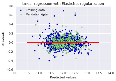
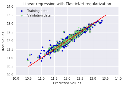
ElasticNet picked 110 features and eliminated the other 209 features
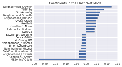
原文:
ElasticNet 在这里使用的最优 L1 比例等于 1,这意味着它与我们之前使用的 Lasso 回归模型完全等价(如果该比例等于 0,则会与我们的岭回归模型完全等价)。模型不需要任何 L2 正则化来克服潜在的 L1 缺陷。
备注:我尝试移除了 “MSZoning_C (all)” 特征,结果本地交叉验证分数略微变差,但公共排行榜分数却略微变好。
结论
投入时间和精力进行数据集预处理并优化正则化,得到了不错的分数,甚至优于一些公开脚本 —— 这些脚本使用的是在 Kaggle 竞赛中历来表现更好的算法,比如随机森林。作为刚接触机器学习竞赛的新手,任何建设性的改进建议我都会非常感激,同时感谢你们花费时间阅读。
三.一些思考总结
1.对可能存在的数据泄露问题的探索
这段代码的顺序是:
- 对整个 train 数据集做:
- 删异常值
- 填充缺失值
- 特征工程(造新特征)
- 计算偏度 + 对数变换
- 独热编码
- 合并所有特征
- 最后才切分 train / test
- 再用训练集拟合标准化,作用于测试集
所有特征工程、填充、对数变换、编码,全都用了「全量数据」的统计信息,然后才拆分训练 / 测试集。
这是 Kaggle 最典型、最常见的数据泄露。
真正的标准流程必须是:
原始数据
    ↓
【第一步:切分 X_train / X_test / y_train / y_test】
    ↓
只在 X_train 上做:
    → 删异常值
    → 业务填充
    → 类别映射
    → 特征工程
    → 计算中位数
    → 计算偏度
    → 对数变换
    → 独热编码
    → 标准化(fit)
    ↓
把所有规则应用到 X_test:
    → transform 绝不 fit
    ↓
训练模型 → 测试集评估 → 提交
2.代码修改
import numpy as np
import pandas as pd
import matplotlib.pyplot as plt
from scipy.stats import skew
from sklearn.model_selection import train_test_split
from sklearn.preprocessing import StandardScaler
from sklearn.metrics import mean_squared_error
from sklearn.metrics import make_scorer
from sklearn.model_selection import cross_val_score
from sklearn.linear_model import LinearRegression, RidgeCV, LassoCV, ElasticNetCV

# ====================== 1. 读取原始数据 ======================
train = pd.read_csv("train.csv")
y = train["SalePrice"]
train = train.drop("SalePrice", axis=1)

# ====================== 【关键】先切分!杜绝一切泄露 ======================
X_train, X_test, y_train, y_test = train_test_split(
    train, y, test_size=0.3, random_state=0
)

# ====================== 2. 异常值处理(仅训练集) ======================
X_train = X_train[X_train.GrLivArea < 4000]
y_train = y_train[X_train.index]

# ====================== 3. 缺失值填充(业务规则,无统计) ======================
def fill_na(df):
    df = df.copy()
    df.loc[:, "Alley"] = df.loc[:, "Alley"].fillna("None")
    df.loc[:, "BedroomAbvGr"] = df.loc[:, "BedroomAbvGr"].fillna(0)
    df.loc[:, "BsmtQual"] = df.loc[:, "BsmtQual"].fillna("No")
    df.loc[:, "BsmtCond"] = df.loc[:, "BsmtCond"].fillna("No")
    df.loc[:, "BsmtExposure"] = df.loc[:, "BsmtExposure"].fillna("No")
    df.loc[:, "BsmtFinType1"] = df.loc[:, "BsmtFinType1"].fillna("No")
    df.loc[:, "BsmtFinType2"] = df.loc[:, "BsmtFinType2"].fillna("No")
    df.loc[:, "BsmtFullBath"] = df.loc[:, "BsmtFullBath"].fillna(0)
    df.loc[:, "BsmtHalfBath"] = df.loc[:, "BsmtHalfBath"].fillna(0)
    df.loc[:, "BsmtUnfSF"] = df.loc[:, "BsmtUnfSF"].fillna(0)
    df.loc[:, "CentralAir"] = df.loc[:, "CentralAir"].fillna("N")
    df.loc[:, "Condition1"] = df.loc[:, "Condition1"].fillna("Norm")
    df.loc[:, "Condition2"] = df.loc[:, "Condition2"].fillna("Norm")
    df.loc[:, "EnclosedPorch"] = df.loc[:, "EnclosedPorch"].fillna(0)
    df.loc[:, "ExterCond"] = df.loc[:, "ExterCond"].fillna("TA")
    df.loc[:, "ExterQual"] = df.loc[:, "ExterQual"].fillna("TA")
    df.loc[:, "Fence"] = df.loc[:, "Fence"].fillna("No")
    df.loc[:, "FireplaceQu"] = df.loc[:, "FireplaceQu"].fillna("No")
    df.loc[:, "Fireplaces"] = df.loc[:, "Fireplaces"].fillna(0)
    df.loc[:, "Functional"] = df.loc[:, "Functional"].fillna("Typ")
    df.loc[:, "GarageType"] = df.loc[:, "GarageType"].fillna("No")
    df.loc[:, "GarageFinish"] = df.loc[:, "GarageFinish"].fillna("No")
    df.loc[:, "GarageQual"] = df.loc[:, "GarageQual"].fillna("No")
    df.loc[:, "GarageCond"] = df.loc[:, "GarageCond"].fillna("No")
    df.loc[:, "GarageArea"] = df.loc[:, "GarageArea"].fillna(0)
    df.loc[:, "GarageCars"] = df.loc[:, "GarageCars"].fillna(0)
    df.loc[:, "HalfBath"] = df.loc[:, "HalfBath"].fillna(0)
    df.loc[:, "HeatingQC"] = df.loc[:, "HeatingQC"].fillna("TA")
    df.loc[:, "KitchenAbvGr"] = df.loc[:, "KitchenAbvGr"].fillna(0)
    df.loc[:, "KitchenQual"] = df.loc[:, "KitchenQual"].fillna("TA")
    df.loc[:, "LotFrontage"] = df.loc[:, "LotFrontage"].fillna(0)
    df.loc[:, "LotShape"] = df.loc[:, "LotShape"].fillna("Reg")
    df.loc[:, "MasVnrType"] = df.loc[:, "MasVnrType"].fillna("None")
    df.loc[:, "MasVnrArea"] = df.loc[:, "MasVnrArea"].fillna(0)
    df.loc[:, "MiscFeature"] = df.loc[:, "MiscFeature"].fillna("No")
    df.loc[:, "MiscVal"] = df.loc[:, "MiscVal"].fillna(0)
    df.loc[:, "OpenPorchSF"] = df.loc[:, "OpenPorchSF"].fillna(0)
    df.loc[:, "PavedDrive"] = df.loc[:, "PavedDrive"].fillna("N")
    df.loc[:, "PoolQC"] = df.loc[:, "PoolQC"].fillna("No")
    df.loc[:, "PoolArea"] = df.loc[:, "PoolArea"].fillna(0)
    df.loc[:, "SaleCondition"] = df.loc[:, "SaleCondition"].fillna("Normal")
    df.loc[:, "ScreenPorch"] = df.loc[:, "ScreenPorch"].fillna(0)
    df.loc[:, "TotRmsAbvGrd"] = df.loc[:, "TotRmsAbvGrd"].fillna(0)
    df.loc[:, "Utilities"] = df.loc[:, "Utilities"].fillna("AllPub")
    df.loc[:, "WoodDeckSF"] = df.loc[:, "WoodDeckSF"].fillna(0)
    return df

X_train = fill_na(X_train)
X_test = fill_na(X_test)

# ====================== 4. 数字转类别(固定映射) ======================
def map_category(df):
    df = df.copy()
    df = df.replace({
        "MSSubClass": {20:"SC20",30:"SC30",40:"SC40",45:"SC45",50:"SC50",60:"SC60",70:"SC70",75:"SC75",
                       80:"SC80",85:"SC85",90:"SC90",120:"SC120",150:"SC150",160:"SC160",180:"SC180",190:"SC190"},
        "MoSold": {1:"Jan",2:"Feb",3:"Mar",4:"Apr",5:"May",6:"Jun",7:"Jul",8:"Aug",9:"Sep",10:"Oct",11:"Nov",12:"Dec"}
    })
    return df

X_train = map_category(X_train)
X_test = map_category(X_test)

# ====================== 5. 有序编码(固定规则) ======================
def map_ordinal(df):
    df = df.copy()
    df = df.replace({
        "Alley": {"Grvl":1,"Pave":2},
        "BsmtCond": {"No":0,"Po":1,"Fa":2,"TA":3,"Gd":4,"Ex":5},
        "BsmtExposure": {"No":0,"Mn":1,"Av":2,"Gd":3},
        "BsmtFinType1": {"No":0,"Unf":1,"LwQ":2,"Rec":3,"BLQ":4,"ALQ":5,"GLQ":6},
        "BsmtFinType2": {"No":0,"Unf":1,"LwQ":2,"Rec":3,"BLQ":4,"ALQ":5,"GLQ":6},
        "BsmtQual": {"No":0,"Po":1,"Fa":2,"TA":3,"Gd":4,"Ex":5},
        "ExterCond": {"Po":1,"Fa":2,"TA":3,"Gd":4,"Ex":5},
        "ExterQual": {"Po":1,"Fa":2,"TA":3,"Gd":4,"Ex":5},
        "FireplaceQu": {"No":0,"Po":1,"Fa":2,"TA":3,"Gd":4,"Ex":5},
        "Functional": {"Sal":1,"Sev":2,"Maj2":3,"Maj1":4,"Mod":5,"Min2":6,"Min1":7,"Typ":8},
        "GarageCond": {"No":0,"Po":1,"Fa":2,"TA":3,"Gd":4,"Ex":5},
        "GarageQual": {"No":0,"Po":1,"Fa":2,"TA":3,"Gd":4,"Ex":5},
        "HeatingQC": {"Po":1,"Fa":2,"TA":3,"Gd":4,"Ex":5},
        "KitchenQual": {"Po":1,"Fa":2,"TA":3,"Gd":4,"Ex":5},
        "LandSlope": {"Sev":1,"Mod":2,"Gtl":3},
        "LotShape": {"IR3":1,"IR2":2,"IR1":3,"Reg":4},
        "PavedDrive": {"N":0,"P":1,"Y":2},
        "PoolQC": {"No":0,"Fa":1,"TA":2,"Gd":3,"Ex":4},
        "Street": {"Grvl":1,"Pave":2},
        "Utilities": {"ELO":1,"NoSeWa":2,"NoSewr":3,"AllPub":4}
    })
    return df

X_train = map_ordinal(X_train)
X_test = map_ordinal(X_test)

# ====================== 6. 特征工程 ======================
def feature_engineering(df):
    df = df.copy()
    df["SimplOverallQual"] = df.OverallQual.replace({1:1,2:1,3:1,4:2,5:2,6:2,7:3,8:3,9:3,10:3})
    df["SimplOverallCond"] = df.OverallCond.replace({1:1,2:1,3:1,4:2,5:2,6:2,7:3,8:3,9:3,10:3})
    df["SimplPoolQC"] = df.PoolQC.replace({1:1,2:1,3:2,4:2})
    df["SimplGarageCond"] = df.GarageCond.replace({1:1,2:1,3:1,4:2,5:2})
    df["SimplGarageQual"] = df.GarageQual.replace({1:1,2:1,3:1,4:2,5:2})
    df["SimplFireplaceQu"] = df.FireplaceQu.replace({1:1,2:1,3:1,4:2,5:2})
    df["SimplFunctional"] = df.Functional.replace({1:1,2:1,3:2,4:2,5:3,6:3,7:3,8:4})
    df["SimplKitchenQual"] = df.KitchenQual
    df["SimplHeatingQC"] = df.HeatingQC
    df["SimplBsmtFinType1"] = df.BsmtFinType1
    df["SimplBsmtFinType2"] = df.BsmtFinType2
    df["SimplBsmtCond"] = df.BsmtCond
    df["SimplBsmtQual"] = df.BsmtQual
    df["SimplExterCond"] = df.ExterCond
    df["SimplExterQual"] = df.ExterQual

    df["OverallGrade"] = df["OverallQual"] * df["OverallCond"]
    df["GarageGrade"] = df["GarageQual"] * df["GarageCond"]
    df["ExterGrade"] = df["ExterQual"] * df["ExterCond"]
    df["KitchenScore"] = df["KitchenAbvGr"] * df["KitchenQual"]
    df["FireplaceScore"] = df["Fireplaces"] * df["FireplaceQu"]
    df["GarageScore"] = df["GarageArea"] * df["GarageQual"]
    df["PoolScore"] = df["PoolArea"] * df["PoolQC"]
    df["SimplOverallGrade"] = df["SimplOverallQual"] * df["SimplOverallCond"]
    df["SimplExterGrade"] = df["SimplExterQual"] * df["SimplExterCond"]
    df["SimplPoolScore"] = df["PoolArea"] * df["SimplPoolQC"]
    df["SimplGarageScore"] = df["GarageArea"] * df["SimplGarageQual"]
    df["SimplFireplaceScore"] = df["Fireplaces"] * df["SimplFireplaceQu"]
    df["SimplKitchenScore"] = df["KitchenAbvGr"] * df["SimplKitchenQual"]
    df["TotalBath"] = df["BsmtFullBath"] + 0.5*df["BsmtHalfBath"] + df["FullBath"] + 0.5*df["HalfBath"]
    df["AllSF"] = df["GrLivArea"] + df["TotalBsmtSF"]
    df["AllFlrsSF"] = df["1stFlrSF"] + df["2ndFlrSF"]
    df["AllPorchSF"] = df["OpenPorchSF"] + df["EnclosedPorch"] + df["3SsnPorch"] + df["ScreenPorch"]
    df["HasMasVnr"] = df.MasVnrType.replace({"BrkCmn":1,"BrkFace":1,"CBlock":1,"Stone":1,"None":0})
    df["BoughtOffPlan"] = df.SaleCondition.replace({"Abnorml":0,"Alloca":0,"AdjLand":0,"Family":0,"Normal":0,"Partial":1})

    for col in ["OverallQual","AllSF","AllFlrsSF","GrLivArea","SimplOverallQual",
                "ExterQual","GarageCars","TotalBath","KitchenQual","GarageScore"]:
        df[col+"-s2"] = df[col] **2
        df[col+"-s3"] = df[col] **3
        df[col+"-Sq"] = np.sqrt(df[col])
    return df

X_train = feature_engineering(X_train)
X_test = feature_engineering(X_test)

# ====================== 7. 分离数值/类别 ======================
categorical_features = X_train.select_dtypes(include=["object"]).columns
numerical_features = X_train.select_dtypes(exclude=["object"]).columns

X_train_num = X_train[numerical_features]
X_test_num = X_test[numerical_features]
X_train_cat = X_train[categorical_features]
X_test_cat = X_test[categorical_features]

# ====================== 8. 中位数填充(仅训练集学习) ======================
train_median = X_train_num.median()
X_train_num = X_train_num.fillna(train_median)
X_test_num = X_test_num.fillna(train_median)

# ====================== 9. 对数变换(仅训练集判断) ======================
skewness = X_train_num.apply(lambda x: skew(x))
skewed_features = skewness[abs(skewness) > 0.5].index

X_train_num[skewed_features] = np.log1p(X_train_num[skewed_features])
X_test_num[skewed_features] = np.log1p(X_test_num[skewed_features])

# ====================== 10. 独热编码(训练+测试统一列) ======================
all_cat = pd.concat([X_train_cat, X_test_cat], axis=0)
all_dummies = pd.get_dummies(all_cat)

X_train_cat = all_dummies.iloc[:len(X_train_cat), :]
X_test_cat = all_dummies.iloc[len(X_train_cat):, :]

# ====================== 11. 合并特征 ======================
X_train_final = pd.concat([X_train_num, X_train_cat], axis=1)
X_test_final = pd.concat([X_test_num, X_test_cat], axis=1)

# ====================== 12. 标准化(仅训练集fit) ======================
stdSc = StandardScaler()
X_train_final.loc[:, numerical_features] = stdSc.fit_transform(X_train_final.loc[:, numerical_features])
X_test_final.loc[:, numerical_features] = stdSc.transform(X_test_final.loc[:, numerical_features])

# ====================== 13. 评估函数 ======================
scorer = make_scorer(mean_squared_error, greater_is_better=False)

def rmse_cv_train(model):
    return np.sqrt(-cross_val_score(model, X_train_final, y_train, scoring=scorer, cv=10))

def rmse_cv_test(model):
    return np.sqrt(-cross_val_score(model, X_test_final, y_test, scoring=scorer, cv=10))

# =============================================================================
# ✅ 以下是全部模型:Linear + Ridge + Lasso + ElasticNet(无泄露版)
# =============================================================================

# ---------------------- 1. Linear Regression ----------------------
lr = LinearRegression()
lr.fit(X_train_final, y_train)

print("RMSE on Training set :", rmse_cv_train(lr).mean())
print("RMSE on Test set :", rmse_cv_test(lr).mean())

y_train_pred = lr.predict(X_train_final)
y_test_pred = lr.predict(X_test_final)

plt.scatter(y_train_pred, y_train_pred - y_train, c="blue", marker="s", label="Training data")
plt.scatter(y_test_pred, y_test_pred - y_test, c="lightgreen", marker="s", label="Validation data")
plt.title("Linear regression")
plt.xlabel("Predicted values")
plt.ylabel("Residuals")
plt.legend(loc="upper left")
plt.hlines(y=0, xmin=10.5, xmax=13.5, color="red")
plt.show()

plt.scatter(y_train_pred, y_train, c="blue", marker="s", label="Training data")
plt.scatter(y_test_pred, y_test, c="lightgreen", marker="s", label="Validation data")
plt.title("Linear regression")
plt.xlabel("Predicted values")
plt.ylabel("Real values")
plt.legend(loc="upper left")
plt.plot([10.5, 13.5], [10.5, 13.5], c="red")
plt.show()

# ---------------------- 2. Ridge ----------------------
ridge = RidgeCV(alphas=[0.01, 0.03, 0.06, 0.1, 0.3, 0.6, 1, 3, 6, 10, 30, 60])
ridge.fit(X_train_final, y_train)
alpha = ridge.alpha_
print("Best alpha :", alpha)

print("Try again for more precision with alphas centered around " + str(alpha))
ridge = RidgeCV(alphas=[alpha * .6, alpha * .65, alpha * .7, alpha * .75, alpha * .8, alpha * .85,
                          alpha * .9, alpha * .95, alpha, alpha * 1.05, alpha * 1.1, alpha * 1.15,
                          alpha * 1.25, alpha * 1.3, alpha * 1.35, alpha * 1.4], cv=10)
ridge.fit(X_train_final, y_train)
alpha = ridge.alpha_
print("Best alpha :", alpha)

print("Ridge RMSE on Training set :", rmse_cv_train(ridge).mean())
print("Ridge RMSE on Test set :", rmse_cv_test(ridge).mean())

y_train_rdg = ridge.predict(X_train_final)
y_test_rdg = ridge.predict(X_test_final)

plt.scatter(y_train_rdg, y_train_rdg - y_train, c="blue", marker="s", label="Training data")
plt.scatter(y_test_rdg, y_test_rdg - y_test, c="lightgreen", marker="s", label="Validation data")
plt.title("Ridge")
plt.xlabel("Predicted values")
plt.ylabel("Residuals")
plt.legend(loc="upper left")
plt.hlines(y=0, xmin=10.5, xmax=13.5, color="red")
plt.show()

plt.scatter(y_train_rdg, y_train, c="blue", marker="s", label="Training data")
plt.scatter(y_test_rdg, y_test, c="lightgreen", marker="s", label="Validation data")
plt.title("Ridge")
plt.xlabel("Predicted values")
plt.ylabel("Real values")
plt.legend(loc="upper left")
plt.plot([10.5, 13.5], [10.5, 13.5], c="red")
plt.show()

coefs = pd.Series(ridge.coef_, index=X_train_final.columns)
print("Ridge picked", sum(coefs != 0), "features and eliminated the other", sum(coefs == 0), "features")
imp_coefs = pd.concat([coefs.sort_values().head(10), coefs.sort_values().tail(10)])
imp_coefs.plot(kind="barh")
plt.title("Ridge Coefficients")
plt.show()

# ---------------------- 3. Lasso ----------------------
lasso = LassoCV(alphas=[0.0001, 0.0003, 0.0006, 0.001, 0.003, 0.006, 0.01, 0.03, 0.06, 0.1, 0.3, 0.6, 1],
                max_iter=50000, cv=10)
lasso.fit(X_train_final, y_train)
alpha = lasso.alpha_
print("Best alpha :", alpha)

print("Try again for more precision with alphas centered around " + str(alpha))
lasso = LassoCV(alphas=[alpha * .6, alpha * .65, alpha * .7, alpha * .75, alpha * .8,
                          alpha * .85, alpha * .9, alpha * .95, alpha, alpha * 1.05,
                          alpha * 1.1, alpha * 1.15, alpha * 1.25, alpha * 1.3, alpha * 1.35, alpha * 1.4],
                max_iter=50000, cv=10)
lasso.fit(X_train_final, y_train)
alpha = lasso.alpha_
print("Best alpha :", alpha)

print("Lasso RMSE on Training set :", rmse_cv_train(lasso).mean())
print("Lasso RMSE on Test set :", rmse_cv_test(lasso).mean())

y_train_las = lasso.predict(X_train_final)
y_test_las = lasso.predict(X_test_final)

plt.scatter(y_train_las, y_train_las - y_train, c="blue", marker="s", label="Training data")
plt.scatter(y_test_las, y_test_las - y_test, c="lightgreen", marker="s", label="Validation data")
plt.title("Lasso")
plt.xlabel("Predicted values")
plt.ylabel("Residuals")
plt.legend(loc="upper left")
plt.hlines(y=0, xmin=10.5, xmax=13.5, color="red")
plt.show()

plt.scatter(y_train_las, y_train, c="blue", marker="s", label="Training data")
plt.scatter(y_test_las, y_test, c="lightgreen", marker="s", label="Validation data")
plt.title("Lasso")
plt.xlabel("Predicted values")
plt.ylabel("Real values")
plt.legend(loc="upper left")
plt.plot([10.5, 13.5], [10.5, 13.5], c="red")
plt.show()

coefs = pd.Series(lasso.coef_, index=X_train_final.columns)
print("Lasso picked", sum(coefs != 0), "features and eliminated the other", sum(coefs == 0), "features")
imp_coefs = pd.concat([coefs.sort_values().head(10), coefs.sort_values().tail(10)])
imp_coefs.plot(kind="barh")
plt.title("Lasso Coefficients")
plt.show()

# ---------------------- 4. ElasticNet ----------------------
elasticNet = ElasticNetCV(l1_ratio=[0.1, 0.3, 0.5, 0.6, 0.7, 0.8, 0.85, 0.9, 0.95, 1],
                          alphas=[0.0001, 0.0003, 0.0006, 0.001, 0.003, 0.006, 0.01, 0.03, 0.06, 0.1, 0.3, 0.6, 1, 3, 6],
                          max_iter=50000, cv=10)
elasticNet.fit(X_train_final, y_train)
alpha = elasticNet.alpha_
ratio = elasticNet.l1_ratio_
print("Best l1_ratio :", ratio)
print("Best alpha :", alpha)

print("Try again for more precision with l1_ratio centered around " + str(ratio))
elasticNet = ElasticNetCV(l1_ratio=[ratio * .85, ratio * .9, ratio * .95, ratio, ratio * 1.05, ratio * 1.1, ratio * 1.15],
                          alphas=[0.0001, 0.0003, 0.0006, 0.001, 0.003, 0.006, 0.01, 0.03, 0.06, 0.1, 0.3, 0.6, 1, 3, 6],
                          max_iter=50000, cv=10)
elasticNet.fit(X_train_final, y_train)
if elasticNet.l1_ratio_ > 1:
    elasticNet.l1_ratio_ = 1
alpha = elasticNet.alpha_
ratio = elasticNet.l1_ratio_
print("Best l1_ratio :", ratio)
print("Best alpha :", alpha)

print("Now try again for more precision on alpha...")
elasticNet = ElasticNetCV(l1_ratio=ratio,
                          alphas=[alpha * .6, alpha * .65, alpha * .7, alpha * .75, alpha * .8, alpha * .85, alpha * .9,
                                  alpha * .95, alpha, alpha * 1.05, alpha * 1.1, alpha * 1.15, alpha * 1.25, alpha * 1.3,
                                  alpha * 1.35, alpha * 1.4],
                          max_iter=50000, cv=10)
elasticNet.fit(X_train_final, y_train)
if elasticNet.l1_ratio_ > 1:
    elasticNet.l1_ratio_ = 1
alpha = elasticNet.alpha_
ratio = elasticNet.l1_ratio_
print("Best l1_ratio :", ratio)
print("Best alpha :", alpha)

print("ElasticNet RMSE on Training set :", rmse_cv_train(elasticNet).mean())
print("ElasticNet RMSE on Test set :", rmse_cv_test(elasticNet).mean())

y_train_ela = elasticNet.predict(X_train_final)
y_test_ela = elasticNet.predict(X_test_final)

plt.scatter(y_train_ela, y_train_ela - y_train, c="blue", marker="s", label="Training data")
plt.scatter(y_test_ela, y_test_ela - y_test, c="lightgreen", marker="s", label="Validation data")
plt.title("ElasticNet")
plt.xlabel("Predicted values")
plt.ylabel("Residuals")
plt.legend(loc="upper left")
plt.hlines(y=0, xmin=10.5, xmax=13.5, color="red")
plt.show()

plt.scatter(y_train, y_train_ela, c="blue", marker="s", label="Training data")
plt.scatter(y_test, y_test_ela, c="lightgreen", marker="s", label="Validation data")
plt.title("ElasticNet")
plt.xlabel("Predicted values")
plt.ylabel("Real values")
plt.legend(loc="upper left")
plt.plot([10.5, 13.5], [10.5, 13.5], c="red")
plt.show()

coefs = pd.Series(elasticNet.coef_, index=X_train_final.columns)
print("ElasticNet picked", sum(coefs != 0), "features and eliminated the other", sum(coefs == 0), "features")
imp_coefs = pd.concat([coefs.sort_values().head(10), coefs.sort_values().tail(10)])
imp_coefs.plot(kind="barh")
plt.title("ElasticNet Coefficients")
plt.show()
3.什么是数据清洗,数据预处理,特征工程,流程的先后顺序是什么?
概念:
1.数据清洗(Data Cleaning)
目的:把脏数据变干净,去掉错误、异常、不合理的数据。
主要做这些事:
- 删除明显异常值(比如房子面积 >4000 这种极端样本)
- 修正错误数据
- 删除重复行
- 处理明显不合理的取值
- 去掉对建模完全没用的列(ID、纯序号等)
2. 数据预处理(Data Preprocessing)
目的:把数据整理成模型能训练的格式。
主要做这些事:
- 填充缺失值(NA → 0、None、众数、中位数)
- 把文本类别转成数字(有序编码、One-Hot)
- 数据标准化 / 归一化(让特征尺度一致)
- 处理偏斜分布(对数变换)
- 数据类型转换
3. 特征工程(Feature Engineering)
目的:从现有数据里 “造” 更有用的信息,让模型更容易学到规律,提升准确率。
主要做这些事:
- 组合特征:面积 × 质量 = 综合评分
- 多项式特征:平方、立方、根号
- 拆分特征:把日期拆成年、月、日
- 统计特征:总和、均值、计数
- 业务特征:是否有车库、是否新房
标准先后顺序:
- 读取数据
- 立刻切分训练集 / 测试集(这一步必须最靠前,否则必泄露)
在训练集上依次做:
- 数据清洗删异常、删错误、删重复
- 数据预处理填充缺失值 → 编码类别 → 处理偏度 → 标准化
- 特征工程造新特征、组合特征、多项式变换
然后把训练集学到的规则应用到测试集:
- 测试集 只做 transform,不做任何学习
- 建模、训练、评估
4.这篇notebook值得学习的点
1.业务理解极强
作者完全读懂了 Ames Housing 数据集的官方文档:
- 知道
NA在很多特征里不是缺失,而是 “没有这个设施”- Alley = NA → 没有小巷
- Garage = NA → 没有车库
- Bsmt = NA → 没有地下室
- 知道哪些是有序特征,哪些是无序分类
- 知道哪些数值其实是分类(MSSubClass、MoSold)
2.有序特征的标准化编码
有序特征怎么编码才能让线性模型学到正确的强弱关系
3.特征工程思路非常强
作者创造的特征:
- TotalBath = 全浴 + 0.5× 半浴
- AllSF = 地上面积 + 地下室面积
- OverallGrade = 质量 × 条件
- GarageScore = 车库面积 × 车库质量
- 各种简化等级、合并等级
- 平方、立方、根号非线性特征
这些不是瞎造,是符合房价逻辑的强特征
4.线性模型 + 正则化 的完整建模流程
Linear → Ridge → Lasso → ElasticNet这套流程是线性模型的标准学习路线。
特别是:
- Lasso 自动做特征选择
- Ridge 收缩系数防过拟合
- ElasticNet 混合两者优点
- 系数可视化看特征重要性
这些都是非常正统、非常专业的建模思路。

AtomGit 是由开放原子开源基金会联合 CSDN 等生态伙伴共同推出的新一代开源与人工智能协作平台。平台坚持“开放、中立、公益”的理念,把代码托管、模型共享、数据集托管、智能体开发体验和算力服务整合在一起,为开发者提供从开发、训练到部署的一站式体验。
更多推荐


 9
9 0
0- 0


 已为社区贡献9条内容

所有评论(0)