✅作者简介：热爱科研的Matlab仿真开发者，擅长毕业设计辅导、数学建模、数据处理、程序设计科研仿真。

🍎完整代码获取 定制创新 论文复现点击：Matlab科研工作室

 👇 关注我领取海量matlab电子书和数学建模资料 

🍊个人信条：做科研，博学之、审问之、慎思之、明辨之、笃行之，是为：博学慎思，明辨笃行。

🔥 内容介绍

一、引言

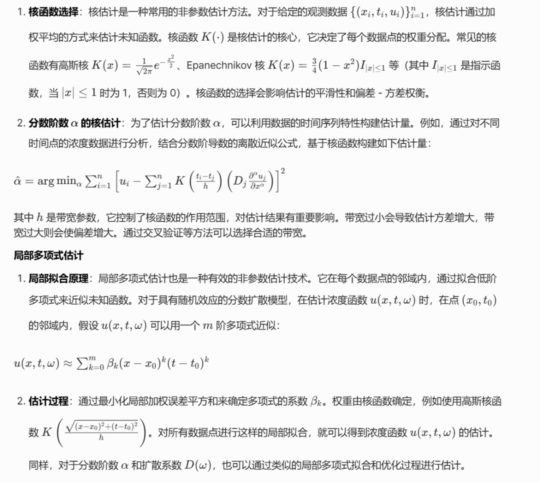
在众多科学和工程领域，如物理、生物、金融等，扩散过程是描述物质或信息传播的重要模型。传统的扩散模型基于整数阶导数，然而，越来越多的研究表明，具有分数阶导数的扩散模型能更好地刻画现实世界中许多复杂的、具有记忆和长程依赖特性的扩散现象。当考虑到环境等因素的不确定性时，引入随机效应来完善分数扩散模型就显得尤为必要。非参数估计方法则为准确推断这类复杂模型的参数和特性提供了有力工具，无需对模型的具体形式做出严格假设，能更灵活地适应数据的内在结构。

二、具有随机效应的分数扩散模型

分数扩散方程基础

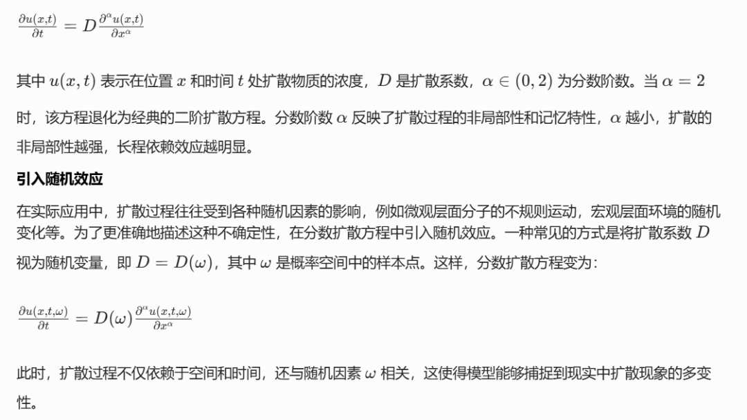
分数扩散方程是对传统扩散方程的拓展，它使用分数阶导数来描述扩散过程。常见的分数阶导数定义有 Caputo、Riemann - Liouville 等。以一维空间的 Caputo 分数阶导数定义的分数扩散方程为例：

⛳️ 运行结果

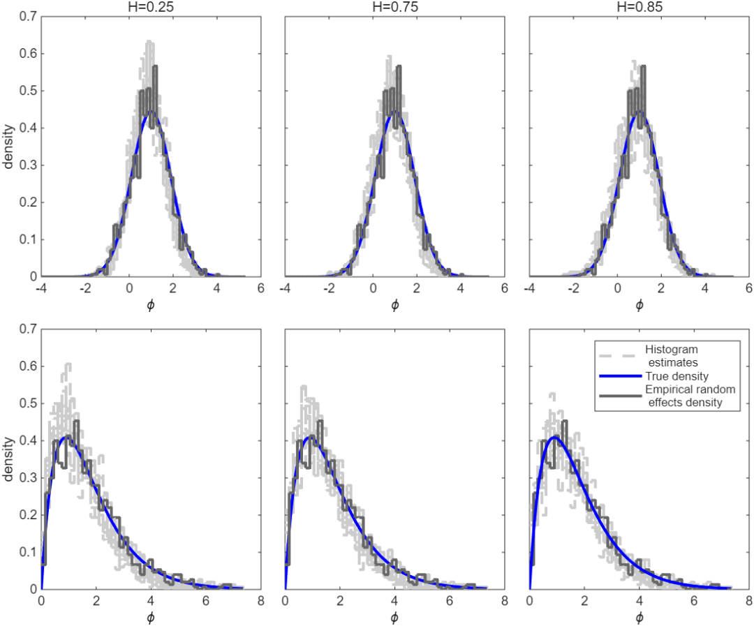
📣 部分代码

function []= printPlots()

%General parameters for the plots

lambda=3*10^(-3);

T=100;

N=1000;

n=2^8;

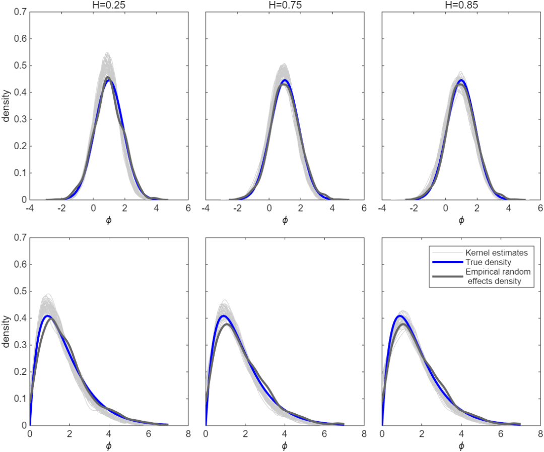
%density plots with H= 0.25 or 0.75 or 0.85

figure

set(gcf,'Units','centimeters','position',[8 5 20 16])

%First plot first row

%Normaldensity mu=1, omc=0.8 and s= 50

subplot('position',[0.07 0.56 0.27 0.4])

PhiHat(T,N,n,1,0.8,lambda,0.25,50)

subplot('position',[0.37 0.56 0.27 0.4])

PhiHat(T,N,n,1,0.8,lambda,0.75,50)

subplot('position',[0.67 0.56 0.27 0.4])

PhiHat(T,N,n,1,0.8,lambda,0.85,50)

%First Plot secound row

%Gammadensity with a1=2, b1=0.9, r= 50 and a= 0 

subplot('position',[0.07 0.08 0.27 0.4])

MixGamma(T,N,n,2,0.9,lambda,0.25,50,0)

subplot('position',[0.37 0.08 0.27 0.4])

MixGamma(T,N,n,2,0.9,lambda,0.75,50,0)

subplot('position',[0.67 0.08 0.27 0.4])

MixGamma(T,N,n,2,0.9,lambda,0.85,50,0)

%Saving these as an png and pdf

saveas(gcf,'density.png')

saveas(gcf,'density.pdf')

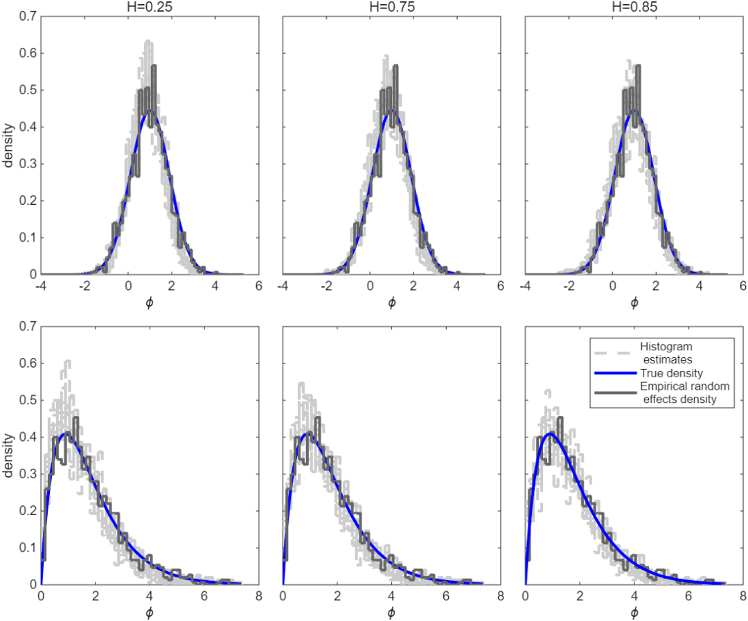
%histogram plots with H = 0.25 or 0.75 or 0.85

figure

set(gcf,'Units','centimeters','position',[8 5 20 16])

%First plot first row

%Normaldistribution mu=1, omc=0.8 and s= 0

subplot('position',[0.07 0.56 0.27 0.4])

histnorm(T,N,n,1,0.8,lambda,0.25,0)

subplot('position',[0.37 0.56 0.27 0.4])

histnorm(T,N,n,1,0.8,lambda,0.75,0)

subplot('position',[0.67 0.56 0.27 0.4])

histnorm(T,N,n,1,0.8,lambda,0.85,0)

%First Plot secound row

%Gammadensity with a1=2, b1=0.9 and a= 0 

subplot('position',[0.07 0.08 0.27 0.4])

histGamma(T,N,n,2,0.9,lambda,0.25,0)

subplot('position',[0.37 0.08 0.27 0.4])

histGamma(T,N,n,2,0.9,lambda,0.75,0)

subplot('position',[0.67 0.08 0.27 0.4])

histGamma(T,N,n,2,0.9,lambda,0.85,0)

%Saving these as an png and pdf

saveas(gcf,'histo.png')

saveas(gcf,'histo.pdf')

🔗 参考文献

🍅更多免费数学建模和仿真教程关注领取