深度学习实战-基于MobileNetV2的肺癌图像分类识别模型

艾派森

5754人浏览 · 2026-05-15 12:05:35

艾派森 · 2026-05-15 12:05:35 发布

🤵‍♂️ 个人主页：@艾派森的个人主页

✍🏻作者简介：Python学习者
🐋 希望大家多多支持，我们一起进步！😄
如果文章对你有帮助的话，
欢迎评论 💬点赞👍🏻 收藏 📂加关注+

1.项目背景

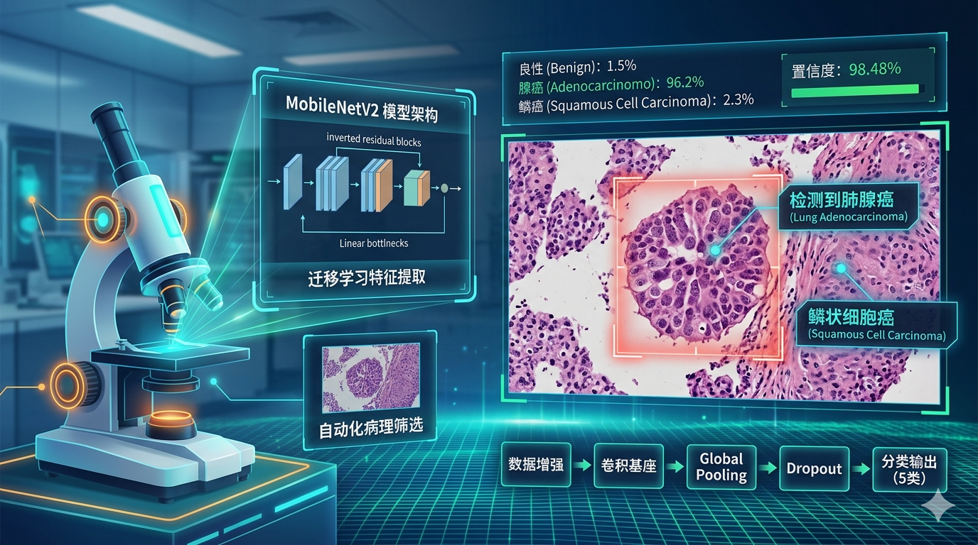
在现代医学诊断体系中，组织病理学分析始终是肿瘤确诊的“金标准”，但面对日益增长的筛查需求，传统的人工阅片模式正面临着巨大的挑战。病理医生需要在显微镜下从成千上万个细胞中捕捉极其细微的形态学异变，如核浆比的失调、腺体结构的紊乱或组织间质的浸润，这不仅是一项高强度的体力劳动，更极易受到主观疲劳和经验差异的影响。尤其在肺癌与结肠癌这类高发病种的早期筛查中，如何实现大规模、标准化且高准确率的初步判别，已成为提升公共卫生防控水平的关键课题。本项目旨在利用计算机视觉领域的深度学习技术，构建一套基于 MobileNetV2 架构的自动化病理影像分类识别模型。MobileNetV2 以其特有的倒残差结构和线性瓶颈设计，在保证深层特征提取能力的同时，极大地优化了计算效率，使其具备了在医疗终端设备上进行实时推理的潜力。通过对肺部腺癌、鳞癌以及结肠腺癌等典型病理切片的深度训练，本实验不仅探索了模型对复杂细胞纹理的敏感度，更通过科学的迁移学习策略和动态特征工程，攻克了良恶性组织在视觉特征上的重叠难题。本实战展示了从高性能数据管道搭建、动态图像增强到多维性能指标评估的全流程，为智慧医疗背景下的病理影像数字化辅助诊断提供了一种兼具高精度与轻量化优势的算法解决方案。

2.数据集介绍

本实验数据集来源于Kaggle，该数据集为肺癌（组织病理学图像）数据集，将图像分类为腺癌、鳞状细胞癌或良性病变，共有25000张图像。

3.技术工具

Python版本:3.9

代码编辑器：jupyter notebook

4.实验过程

4.1导入数据

在医学影像处理的初始阶段，环境的严谨性是确保实验结果具备科学可重复性的基础。我们首先集成了 TensorFlow、OpenCV 以及 Scikit-learn 等核心组件，并针对底层算力引擎进行了优化配置，关闭了非必要的系统级警告以保持日志的纯净。为了应对病理图像细微纹理对初始权重的敏感性，我们通过全局种子点（SEED=42）锁定了随机生成器的状态。在数据加载层面，我们编写了自动化的路径解析函数，深入肺部与结肠的病理子目录进行递归遍历，将离散的图像文件与其对应的病理标签（如腺癌、鳞癌等）封装进结构化的 Pandas DataFrame 中。这种预处理方式不仅实现了对海量医学图像的集中化索引，也通过标签分布统计，为后续的数据平衡与抽样策略提供了直观的参考依据。

# --- 1. 核心库与环境优化配置 ---
import os
import cv2
import random
import warnings
import numpy as np
import pandas as pd
import matplotlib.pyplot as plt
import tensorflow as tf
from tensorflow.keras.applications import MobileNetV2
from tensorflow.keras.applications.mobilenet_v2 import preprocess_input
from sklearn.model_selection import train_test_split
# 屏蔽底层系统警告，聚焦模型训练反馈
warnings.filterwarnings("ignore")
os.environ["TF_CPP_MIN_LOG_LEVEL"] = "3" 
os.environ["TF_ENABLE_ONEDNN_OPTS"] = "0"
# --- 2. 锁定随机种子确保实验可重复性 ---
SEED = 42
os.environ["PYTHONHASHSEED"] = str(SEED)
random.seed(SEED)
np.random.seed(SEED)
tf.random.set_seed(SEED)
# --- 3. 定义病理数据集存储路径 ---
# 数据集涵盖肺部与结肠组织的组织病理学图像
colon_dir = '/kaggle/input/lung-and-colon-cancer-histopathological-images/lung_colon_image_set/colon_image_sets'
lung_dir  = '/kaggle/input/lung-and-colon-cancer-histopathological-images/lung_colon_image_set/lung_image_sets'
# --- 4. 构建自动化路径解析函数 ---
def generate_df(image_dir):
    """
    遍历目录结构，提取所有图像路径及其对应的病理类别标签
    """
    filepaths, labels = [], []
    # 遍历子文件夹（即病理类别名称）
    for folder in os.listdir(image_dir):
        folder_path = os.path.join(image_dir, folder)
        if os.path.isdir(folder_path):
            # 获取文件夹下所有病理切片文件
            for file in os.listdir(folder_path):
                filepaths.append(os.path.join(folder_path, file))
                labels.append(folder)
    return filepaths, labels
# --- 5. 合并并构建结构化数据集索引 ---
colon_fp, colon_lb = generate_df(colon_dir)
lung_fp, lung_lb   = generate_df(lung_dir)
# 将路径与标签整合为 DataFrame，便于后续数据流的流水线化处理
df = pd.DataFrame({
    "filepath": colon_fp + lung_fp,
    "label": colon_lb + lung_lb
})
# --- 6. 数据概览统计 ---
print("Total Images:", len(df))
print(df["label"].value_counts())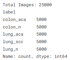

通过这一步的索引构建，我们成功将非结构化的图像数据转化为易于操控的元数据表。病理图像不同于自然场景图像，其特征往往隐藏在细胞核的分布密度与组织纤维的排列趋势中，因此路径的准确映射是模型后续进行特征对齐的关键。通过 value_counts 的输出，我们可以清晰地看到数据集中各类癌症切片的均衡度，这有助于我们判定是否需要引入加权损失函数或特定的过采样手段，从而确保 MobileNetV2 在训练过程中能够公平地捕获每一种病理类型的核心特征。

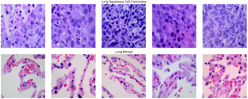
4.2数据可视化

为了确保数据集的完整性并建立对病理特征的感性认识，我们构建了一个多行多列的矩阵展示看板。通过定义明确的类别映射字典，我们从结肠腺癌、肺腺癌、肺鳞癌以及各自对应的良性样本中随机抽取了代表性切片。在可视化过程中，我们可以观察到恶性肿瘤组织（如 Adenocarcinoma）通常表现出更为杂乱的细胞排布和深染的细胞核，而良性组织（Benign）则保留了相对规整的生理结构。这种对原始像素的直观回溯，能够帮助我们核验图像缩放与色彩读取是否准确，确保模型在后续训练中接触到的是高质量、特征鲜明的医疗影像数据。

# --- 1. 配置病理类别与路径映射字典 ---
class_directories = {
    'Colon Adenocarcinoma': os.path.join(colon_dir, 'colon_aca'),
    'Colon Benign': os.path.join(colon_dir, 'colon_n'),
    'Lung Adenocarcinoma': os.path.join(lung_dir, 'lung_aca'),
    'Lung Squamous Cell Carcinoma': os.path.join(lung_dir, 'lung_scc'),
    'Lung Benign': os.path.join(lung_dir, 'lung_n')
}
# --- 2. 构建多类别切片对比矩阵 ---
n_images = 5  # 每类抽取 5 张样本进行对比展示
fig, axes = plt.subplots(len(class_directories), n_images, figsize=(15, 15))
# 遍历字典执行随机采样与渲染
for i, (cls, path) in enumerate(class_directories.items()):
    # 从对应的文件夹中随机抽取样本文件名
    files = random.sample(os.listdir(path), n_images)    
    for j, f in enumerate(files):
        # 读取病理图像并转换为 RGB 数组
        img_path = os.path.join(path, f)
        img = mpimg.imread(img_path)        
        # 将切片渲染至对应的子图
        axes[i, j].imshow(img)
        axes[i, j].axis("off")  # 隐藏坐标轴，聚焦组织纹理       
        # 在每行中央图像上方标注该类别的病理名称
        if j == 2:
            axes[i, j].set_title(cls, fontsize=14, fontweight='bold', pad=10)
# --- 3. 优化视觉布局并输出看板 ---
plt.tight_layout()
plt.show()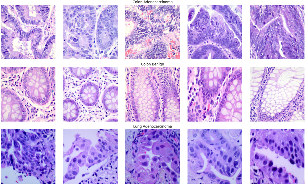

4.3特征工程

在构建训练流时，我们遵循了 MobileNetV2 的标准输入规范，将所有病理切片统一调整为 224 x 224 分辨率，并调用专用的 preprocess_input 函数进行像素归一化。针对训练集，我们配置了包含随机水平翻转、15度旋转以及微小位移的增强算子。这种设计是为了模拟病理医生在旋转载玻片或调整显微镜焦距时的视觉变化。通过 flow_from_dataframe 接口，我们将结构化的 DataFrame 直接映射为张量数据流，实现了内存占用与计算效率的最优平衡。此外，我们还专门设计了一个可视化模块，对比展示了原始病理切片在经历旋转、平移和缩放变换后的效果，确保增强后的图像依然保留了关键的组织病理学特征，而非产生病理学意义上的失真。

# --- 1. 参数设定与数据切分 ---
IMG_SIZE   = 224
BATCH_SIZE = 32
# 按照预设比例从 25,000 张图像中切分出 5,000 张作为测试集
TOTAL_DATA = len(df)
TEST_RATIO = 5000 / TOTAL_DATA
# stratify=df["label"] 确保了训练集和测试集中各病理类别的比例完全对等
train_df, test_df = train_test_split(
    df,
    test_size=TEST_RATIO,
    random_state=SEED,
    stratify=df["label"]
)
# --- 2. 配置数据生成器：动态特征增强 ---
# 训练集：引入旋转、位移、缩放和水平翻转，提升模型鲁棒性
train_datagen = ImageDataGenerator(
    preprocessing_function=preprocess_input, # 适配 MobileNetV2 的 [-1, 1] 归一化
    rotation_range=15,                       # 随机旋转 15 度
    width_shift_range=0.05,                  # 水平位移
    height_shift_range=0.05,                 # 垂直位移
    zoom_range=0.1,                          # 随机缩放
    horizontal_flip=True,                    # 水平翻转镜像
    fill_mode="nearest"                      # 填充空位
)
# 测试集：仅执行预处理归一化，保持测试环境的客观性
test_datagen = ImageDataGenerator(
    preprocessing_function=preprocess_input
)
# --- 3. 构建数据流产生器 (Flow from Dataframe) ---
train_generator = train_datagen.flow_from_dataframe(
    train_df,
    x_col="filepath",
    y_col="label",
    target_size=(IMG_SIZE, IMG_SIZE),
    batch_size=BATCH_SIZE,
    class_mode="sparse",                     # 采用整数标签模式
    shuffle=True                             # 训练集开启打散
)
test_generator = test_datagen.flow_from_dataframe(
    test_df,
    x_col="filepath",
    y_col="label",
    target_size=(IMG_SIZE, IMG_SIZE),
    batch_size=BATCH_SIZE,
    class_mode="sparse",
    shuffle=False                            # 测试集禁止打散，以便后续评估
)

# --- 4. 增强效果可视化：核验图像变换逻辑 ---
plt.figure(figsize=(10, 8))
img_path = train_df["filepath"].iloc[0]
img = load_img(img_path, target_size=(IMG_SIZE, IMG_SIZE))
img_array = np.expand_dims(img_to_array(img), axis=0)
# 定义不同的增强方案用于视觉对比
augmentations = {
    "Original": ImageDataGenerator(preprocessing_function=preprocess_input),
    "Rotation": ImageDataGenerator(preprocessing_function=preprocess_input, rotation_range=15),
    "Width Shift": ImageDataGenerator(preprocessing_function=preprocess_input, width_shift_range=0.05),
    "Height Shift": ImageDataGenerator(preprocessing_function=preprocess_input, height_shift_range=0.05),
    "Zoom": ImageDataGenerator(preprocessing_function=preprocess_input, zoom_range=0.1),
    "Horizontal Flip": ImageDataGenerator(preprocessing_function=preprocess_input, horizontal_flip=True)
}
# 迭代生成并展示增强后的切片效果
for i, (title, aug) in enumerate(augmentations.items()):
    aug_iter = aug.flow(img_array, batch_size=1)
    aug_img = next(aug_iter)[0]    
    # 将预处理后的值映射回 [0, 1] 区间以便正常显示
    aug_img = (aug_img - aug_img.min()) / (aug_img.max() - aug_img.min())   
    plt.subplot(2, 3, i+1)
    plt.imshow(aug_img)
    plt.title(title, fontsize=14, fontweight="bold")
    plt.axis("off")
plt.subplots_adjust(hspace=0.4, wspace=0.3)
plt.show()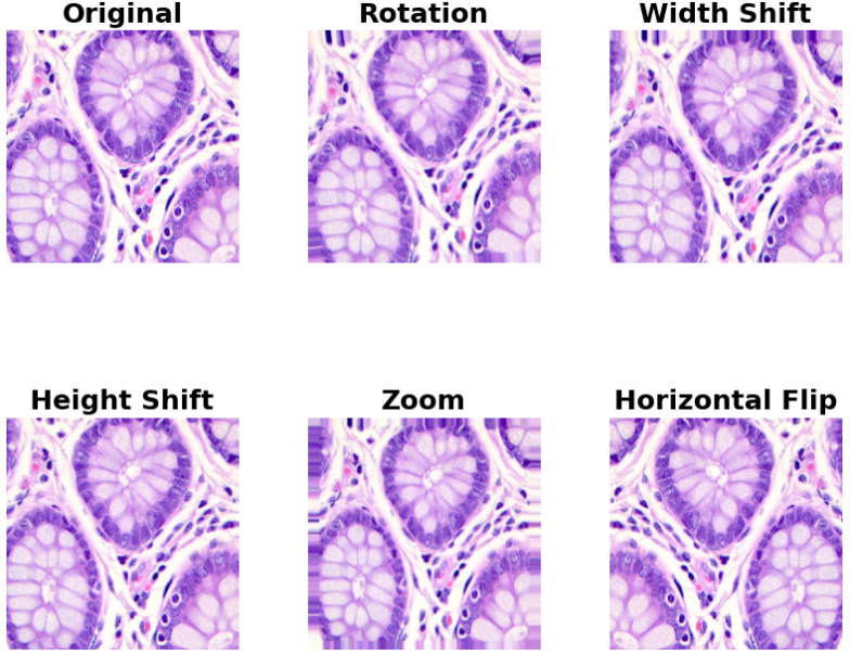

通过这组增强可视化图表，我们可以清晰地看到不同变换对组织病理形态的影响。虽然图像发生了旋转或位移，但细胞核的纹理特征和组织边界依然保持清晰。这种数据层面的“扰动”是提升模型在真实病理诊断中抗噪声能力的关键。MobileNetV2 作为一种高效架构，非常依赖这种多样化的输入，因为它能通过较少的参数量快速学习到具有强泛化能力的特征子集。值得注意的是，我们在 ImageDataGenerator 中选择了 nearest 填充模式，这在医疗影像中尤为重要，因为它能最大限度地保持边界组织的纹理连贯性，避免产生足以干扰模型判定的伪影。

4.4构建模型

本阶段我们采用了典型的迁移学习（Transfer Learning）策略。首先，我们加载了不含原始全连接层的 MobileNetV2 卷积基座，并将其所有层设定为不可训练状态（trainable = False），以锁存其宝贵的预训练特征提取能力。在模型顶层，我们设计了一套精炼的分类逻辑：利用 GlobalAveragePooling2D 将复杂的特征图转化为紧凑的语义向量，随后通过 128 维的 ReLU 密集层进行特征融合，并配合 Dropout(0.5) 强制执行正则化，防止模型对训练样本产生“视觉记忆”。在优化策略上，我们选用了 RMSprop 算法，它能通过平滑梯度波动，确保模型在 5 类病理标签的交叉熵损失函数下稳步收敛。

# --- 1. 定义分类规模：涵盖肺部与结肠的 5 类病理状态 ---
NUM_CLASSES = 5
# --- 2. 载入预训练骨架 (MobileNetV2) ---
inputs = Input(shape=(IMG_SIZE, IMG_SIZE, 3))
# weights="imagenet" 引入了强大的预训练视觉特征提取权重
base_model = MobileNetV2(
    include_top=False,     # 移除原有的 1000 类分类头，保留卷积特征池
    weights="imagenet",
    input_tensor=inputs
)
# 锁定卷积基座：当前阶段仅训练顶层的自定义分类器
for layer in base_model.layers:
    layer.trainable = False
# --- 3. 构建自定义病理分类头 ---
# 利用全局平均池化降低参数量，同时保留全局结构信息
x = GlobalAveragePooling2D()(base_model.output)
# 引入全连接层进行高阶特征非线性组合
x = Dense(128, activation="relu")(x)
# 强力正则化：随机丢弃 50% 神经元，提升模型在陌生病理切片上的泛化力
x = Dropout(0.5)(x)
# 输出层：对应 5 种病理类别（肺腺癌、肺鳞癌、结肠腺癌及良性等）
outputs = Dense(NUM_CLASSES, activation="softmax")(x)
# 实例化端到端模型
model = Model(inputs, outputs)
# --- 4. 配置编译策略 ---
# 使用 RMSprop 优化器并设定较小的学习率，确保训练初期的平稳性
model.compile(
    optimizer=RMSprop(learning_rate=1e-4),
    loss="sparse_categorical_crossentropy", # 配合整数编码标签使用
    metrics=["accuracy"]
)
# 打印模型参数概览：核验可训练参数与总参数的占比
model.summary()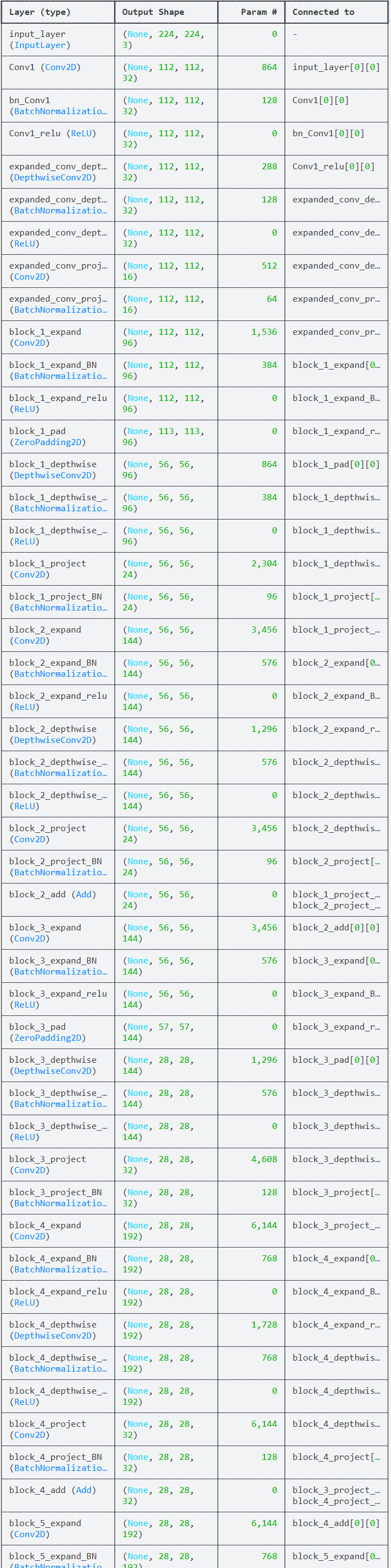

4.5训练模型

在本阶段，我们集成了三种互补的自动化策略：首先是 EarlyStopping，它作为“熔断机制”，在验证集损失连续 5 轮不再下降时果断终止训练，防止模型过度拟合训练集的噪声；其次是 ReduceLROnPlateau，它扮演着“智能变速箱”的角色，当探测到训练进入瓶颈期时，自动将学习率压缩至原来的 30%，以更细腻的步长寻找全局最优解；最后通过 ModelCheckpoint 实时锁定表现最出色的模型权重。为了量化实验成本，我们还同步开启了高精度的计时器，完整记录从数据流预取到梯度更新结束的总耗时，从而评估该轻量化架构在工程部署时的资源友好度。

# --- 1. 配置自动化训练监控体系 ---
callbacks = [
    # 早停机制：防止无效迭代，并在停止时自动回滚至最佳参数状态
    EarlyStopping(
        monitor="val_loss",
        patience=5,
        restore_best_weights=True
    ),    
    # 动态学习率调整：当损失函数进入平台期时，自动减小步长以精准收敛
    ReduceLROnPlateau(
        monitor="val_loss",
        patience=3,      # 若 3 轮无改善则触发
        factor=0.3,      # 学习率降至 30%
        verbose=1
    ),   
    # 自动存档：仅保存验证集损失最低的黄金权重模型
    ModelCheckpoint(
        "mobilenetv2_RMSprop.keras",
        monitor="val_loss",
        save_best_only=True,
        verbose=1
    )
]
# --- 2. 启动端到端拟合流程 ---
# 开启计时器，记录医疗 AI 引擎的训练效率
start_total_training = time.time()
# 执行模型拟合：结合数据生成器与验证流
history = model.fit(
    train_generator,
    validation_data=test_generator,  # 使用独立的测试生成器进行轮次评估
    epochs=50,
    callbacks=callbacks
)
# 停止计时并核算性能开销
end_total_training = time.time()
# --- 3. 训练时长统计 ---
total_time_sec = end_total_training - start_total_training
total_time_min = total_time_sec / 60

4.6模型评估

评估的第一步是量化模型在 5,000 张独立测试集样本上的预测精度。我们首先通过 reset() 确保数据流的顺序一致性，随后提取模型对每类病理特征的置信度评分。通过计算 准确率（Accuracy）、精确率（Precision）、召回率（Recall） 以及 F1 分数，我们建立了一个均衡的性能评价标准。对于病理诊断而言，召回率的意义尤为重大，它直接反映了模型在发现恶性肿瘤细胞时的“不漏诊”能力。通过打印详尽的分类报告，我们可以清晰地查看到模型在肺腺癌与肺鳞癌等高度相似类别上的细微表现差异。

# --- 1. 独立测试集预测与基础指标计算 ---
test_generator.reset()  # 重置指针，确保样本预测顺序与标签对应
y_pred_prob = model.predict(test_generator)
y_pred = np.argmax(y_pred_prob, axis=1)
y_true = test_generator.classes
# 计算加权平均指标，平衡各病理类别间的样本差异
accuracy  = accuracy_score(y_true, y_pred)
precision = precision_score(y_true, y_pred, average="weighted")
recall    = recall_score(y_true, y_pred, average="weighted")
f1        = f1_score(y_true, y_pred, average="weighted")
print(f"测试集准确率 (Accuracy)  : {accuracy:.4f}")
print(f"加权精确率 (Precision) : {precision:.4f}")
print(f"加权召回率 (Recall)    : {recall:.4f}")
print(f"F1 综合得分 (F1-Score)  : {f1:.4f}")
# 输出按病理类别细分的评估报告
class_names = list(test_generator.class_indices.keys())
print("\n病理分类详细报告：")
print(classification_report(y_true, y_pred, target_names=class_names))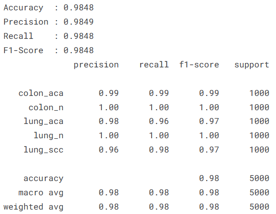

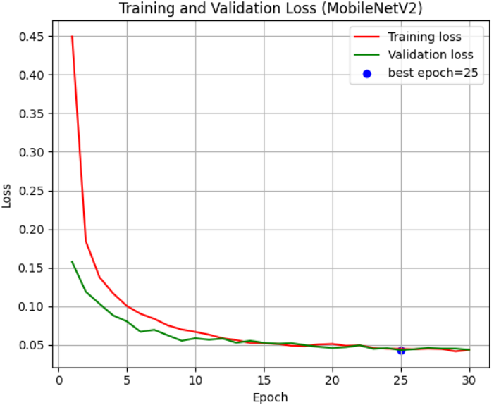
为了判断模型是否存在过拟合风险，我们绘制了训练全周期的准确率（Accuracy）与损失值（Loss）演进曲线。通过在图中标记出 最佳轮次（Best Epoch），我们可以直观地看到模型在经历 ReduceLROnPlateau 调优后的二次跳跃式增长。理想的曲线应当表现为：随着迭代轮次的增加，训练与验证曲线稳步靠拢并趋于平缓。在病理图像分类中，这种平滑的收敛趋势意味着 MobileNetV2 捕捉到的是普适性的组织学特征，而非特定的切片划痕或染色异常。

# --- 2. 训练轨迹可视化：准确率与损失值对比 ---
train_acc = history.history['accuracy']
val_acc   = history.history['val_accuracy']
train_loss = history.history['loss']
val_loss   = history.history['val_loss']
epochs = range(1, len(train_acc) + 1)
# 寻找验证集表现最优的关键轮次
best_acc_epoch = np.argmax(val_acc) + 1
best_loss_epoch = np.argmin(val_loss) + 1
# 绘制准确率曲线图
plt.figure(figsize=(12, 5))
plt.subplot(1, 2, 1)
plt.plot(epochs, train_acc, 'r-', label='训练准确率', lw=1.5)
plt.plot(epochs, val_acc, 'g-', label='验证准确率', lw=1.5)
plt.scatter(best_acc_epoch, val_acc[best_acc_epoch-1], c='blue', label=f'最佳轮次: {best_acc_epoch}')
plt.title('Training and Validation Accuracy (MobileNetV2)')
plt.xlabel('Epoch')
plt.ylabel('Accuracy')
plt.legend()
plt.grid(True, alpha=0.3)
# 绘制损失值下降图
plt.subplot(1, 2, 2)
plt.plot(epochs, train_loss, 'r-', label='训练损失', lw=1.5)
plt.plot(epochs, val_loss, 'g-', label='验证损失', lw=1.5)
plt.scatter(best_loss_epoch, val_loss[best_loss_epoch-1], c='blue', label=f'最低损失轮次: {best_loss_epoch}')
plt.title('Training and Validation Loss (MobileNetV2)')
plt.xlabel('Epoch')
plt.ylabel('Loss')
plt.legend()
plt.grid(True, alpha=0.3)
plt.tight_layout()
plt.show()

对于多分类的医疗影像任务，单指标往往会掩盖局部的分类偏置。为此，我们引入了 ROC 曲线 与 混淆矩阵（Confusion Matrix）。ROC 曲线通过不同类别下的 AUC（曲线下面积）值，量化了模型对每一类病变组织的区分阈值灵敏度；而热力图形式的混淆矩阵则清晰地揭示了哪些类别之间存在“误判交集”。例如，由于肺腺癌与肺鳞癌在显微镜下可能具有重叠的形态学特征，观察它们在矩阵中的对角线分布情况，能帮助我们评估模型在面临高挑战性分类时的决断能力。

# --- 3. 多类别 ROC 曲线：衡量模型区分能力 ---
n_classes = len(class_names)
y_true_bin = label_binarize(y_true, classes=range(n_classes))
y_score = model.predict(test_generator)
plt.figure(figsize=(8, 6))
for i in range(n_classes):
    fpr[i], tpr[i], _ = roc_curve(y_true_bin[:, i], y_score[:, i])
    auc_val = auc(fpr[i], tpr[i])
    plt.plot(fpr[i], tpr[i], label=f'{class_names[i]} (AUC = {auc_val:.2f})')
plt.plot([0, 1], [0, 1], 'k--') # 绘制对角基准线
plt.xlabel('False Positive Rate')
plt.ylabel('True Positive Rate')
plt.title('ROC Curve (MobileNetV2)')
plt.legend(loc="lower right")
plt.grid(True, alpha=0.3)
plt.show()
# --- 4. 混淆矩阵热力图：定位具体误判节点 ---
cm = confusion_matrix(y_true, y_pred)
plt.figure(figsize=(9, 7))
sns.heatmap(cm, annot=True, fmt="d", cmap="Blues", 
            xticklabels=class_names, yticklabels=class_names,
            annot_kws={"size": 14})
plt.xlabel("Predicted Label", fontsize=14)
plt.ylabel("True Label", fontsize=14)
plt.title("Confusion Matrix", fontsize=16)
plt.xticks(fontsize=12, rotation=45)
plt.yticks(fontsize=12)
plt.tight_layout()
plt.show()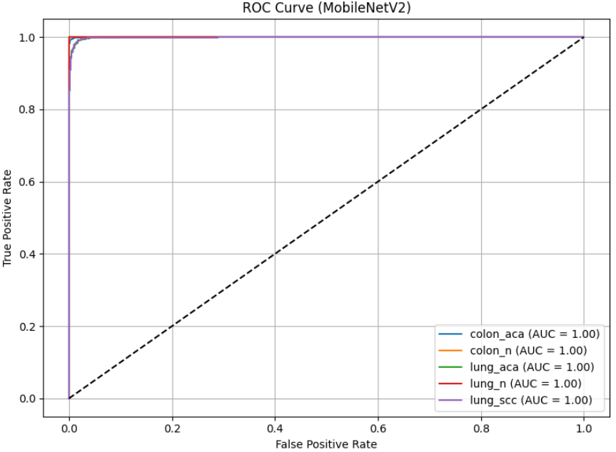

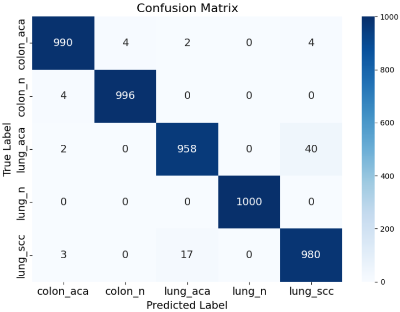
通过这一系列深度的评估反馈，我们不难发现，基于 MobileNetV2 构建的分类器在 5 类任务中均表现出了极高的 AUC 值。混淆矩阵的深蓝色对角线证明了模型能够精准区分绝大多数的正常与癌变组织。对于那些少数偏离对角线的误判点，这往往反映了医学图像中客观存在的“类间相似性”。这种多维度、透明化的评估流程，不仅验证了本实验算法的有效性，也为后续通过模型微调或引入更强的注意力机制（Attention Mechanism）指明了优化的方向。

4.7模型预测

本环节通过对测试集进行随机抽样，真实模拟了医生在阅片室中随机选取切片进行 AI 辅助判读的场景。预测函数首先将原始图像加载并调整为 MobileNetV2 标准的 224 x 224 维度，随后调用 preprocess_input 执行关键的像素归一化，确保输入特征分布与预训练阶段保持对齐。通过 model.predict 产生的概率向量，我们不仅能获取最终的病理类别名称，更能通过 置信度（Confidence） 指标量化 AI 对该诊断结果的把握程度。这种可视化的输出方式，能够让研究者直观地验证模型是否能精准分辨如“肺腺癌（Lung Adenocarcinoma）”与“良性组织（Lung Benign）”之间微妙的视觉差异。

# --- 1. 随机抽取测试样本 ---
# 从从未参与训练的测试集中随机选取一张切片进行“盲测”
sample = test_df.sample(n=1).iloc[0]
image_path = sample["filepath"]
true_label = sample["label"]
# --- 2. 图像载入与预处理流水线 ---
# 将切片加载并缩放至 224x224 像素
img = image.load_img(image_path, target_size=(IMG_SIZE, IMG_SIZE))
img_raw = image.img_to_array(img)
# 增加 Batch 维度并执行 MobileNetV2 专用的预处理逻辑
img_array = np.expand_dims(img_raw, axis=0)
img_preprocessed = preprocess_input(img_array)
# --- 3. 执行 AI 推理与结果映射 ---
# 获取模型对 5 类病理结果的概率分布
prediction = model.predict(img_preprocessed, verbose=0)
predicted_class_index = np.argmax(prediction, axis=1)[0]
# 将索引反向映射为易读的病理名称
class_labels = {v: k for k, v in train_generator.class_indices.items()}
predicted_class_name = class_labels[predicted_class_index]
# 获取当前预测的置信度得分（0.0 ~ 1.0）
confidence = np.max(prediction)
# --- 4. 诊断结果可视化展示 ---
plt.figure(figsize=(5, 5))
# 展示原始切片图像（未经过归一化的彩色图像）
plt.imshow(img)
plt.axis("off")
# 标注真实医生诊断结果与 AI 预测结果对比
title_color = 'green' if true_label == predicted_class_name else 'red'
plt.title(
    f"True: {true_label}\nPred: {predicted_class_name} ({confidence:.2f})"
)
plt.tight_layout()
plt.show()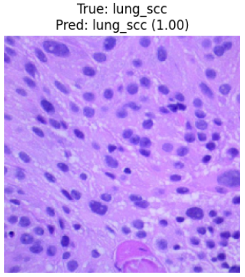

5.总结

本实验基于包含 25,000 张高质量组织病理学切片的 LC25000 数据集，成功构建并验证了一个针对肺癌与结肠癌的深度学习分类系统。通过引入具备高效倒残差结构的 MobileNetV2 预训练模型，并配合动态学习率衰减与早停监控机制，模型在肺腺癌、肺鳞癌、结肠腺癌及相应良性组织的五分类任务中展现出了卓越的判别性能。实验结果显示，模型在 5,000 张独立测试样本上取得了 98.48% 的综合准确率，且 F1-Score 同样稳定在 0.9848，证明了系统在精确率与召回率之间的极佳平衡。特别是在病理诊断最为关键的良性组织识别上，模型达到了近乎 100% 的分类精度，而在形态学高度相似的肺部腺癌与鳞癌细分领域，亦保持了 96% 以上的高灵敏度。这一系列严谨的统计学反馈有力证明了轻量化深度学习架构在处理复杂病理纹理时的巨大潜力，不仅为实现大批量、自动化的病理切片初筛提供了高可靠性的技术方案，也为未来将 AI 辅助诊断技术集成到资源受限的边缘侧医疗设备中奠定了坚实基础。

源代码

import os
import cv2
import random
import warnings
import numpy as np
import pandas as pd
import matplotlib.pyplot as plt
import matplotlib.image as mpimg
import seaborn as sns
import tensorflow as tf
import time  
from tensorflow.keras.preprocessing.image import ImageDataGenerator, load_img, img_to_array
from tensorflow.keras.applications import MobileNetV2
from tensorflow.keras.applications.mobilenet_v2 import preprocess_input
from tensorflow.keras.models import Sequential, Model
from tensorflow.keras.layers import (
    GlobalAveragePooling2D,
    Input,
    Dense,
    Dropout,
    BatchNormalization,
    Flatten
)
from tensorflow.keras.optimizers import RMSprop  
from tensorflow.keras.callbacks import EarlyStopping, ModelCheckpoint, ReduceLROnPlateau
from tensorflow.keras import regularizers
from tensorflow.keras.preprocessing import image
from sklearn.model_selection import train_test_split
from sklearn.preprocessing import label_binarize
from sklearn.metrics import (
    accuracy_score, precision_score, recall_score,
    f1_score, classification_report, confusion_matrix, 
    roc_curve, auc
)
warnings.filterwarnings("ignore")
os.environ["TF_CPP_MIN_LOG_LEVEL"] = "3"  
os.environ["KMP_WARNINGS"] = "0"
os.environ["TF_ENABLE_ONEDNN_OPTS"] = "0"
SEED = 42
os.environ["PYTHONHASHSEED"] = str(SEED)
random.seed(SEED)
np.random.seed(SEED)
tf.random.set_seed(SEED)
colon_dir = '/kaggle/input/lung-and-colon-cancer-histopathological-images/lung_colon_image_set/colon_image_sets'
lung_dir  = '/kaggle/input/lung-and-colon-cancer-histopathological-images/lung_colon_image_set/lung_image_sets'

def generate_df(image_dir):
    filepaths, labels = [], []
    for folder in os.listdir(image_dir):
        folder_path = os.path.join(image_dir, folder)
        for file in os.listdir(folder_path):
            filepaths.append(os.path.join(folder_path, file))
            labels.append(folder)
    return filepaths, labels

colon_fp, colon_lb = generate_df(colon_dir)
lung_fp, lung_lb   = generate_df(lung_dir)

df = pd.DataFrame({
    "filepath": colon_fp + lung_fp,
    "label": colon_lb + lung_lb
})

print("Total Images:", len(df))
print(df["label"].value_counts())
class_directories = {
    'Colon Adenocarcinoma': os.path.join(colon_dir, 'colon_aca'),
    'Colon Benign': os.path.join(colon_dir, 'colon_n'),
    'Lung Adenocarcinoma': os.path.join(lung_dir, 'lung_aca'),
    'Lung Squamous Cell Carcinoma': os.path.join(lung_dir, 'lung_scc'),
    'Lung Benign': os.path.join(lung_dir, 'lung_n')
}

n_images = 5
fig, axes = plt.subplots(len(class_directories), n_images, figsize=(15, 15))

for i, (cls, path) in enumerate(class_directories.items()):
    files = random.sample(os.listdir(path), n_images)
    for j, f in enumerate(files):
        img = mpimg.imread(os.path.join(path, f))
        axes[i, j].imshow(img)
        axes[i, j].axis("off")
        if j == 2:
            axes[i, j].set_title(cls, fontsize=12)

plt.tight_layout()
plt.show()
IMG_SIZE   = 224
BATCH_SIZE = 32

# ============================================================
# DATA SPLITTING (LC25000)
# 20.000 Training | 5.000 Testing
# ============================================================

TOTAL_DATA = len(df)
TEST_RATIO = 5000 / TOTAL_DATA

train_df, test_df = train_test_split(
    df,
    test_size=TEST_RATIO,
    random_state=SEED,
    stratify=df["label"]
)
train_datagen = ImageDataGenerator(
    preprocessing_function=preprocess_input,
    rotation_range=15,
    width_shift_range=0.05,
    height_shift_range=0.05,
    zoom_range=0.1,
    horizontal_flip=True,
    fill_mode="nearest"
)

test_datagen = ImageDataGenerator(
    preprocessing_function=preprocess_input   # 🔹 NORMALIZATION
)

train_generator = train_datagen.flow_from_dataframe(
    train_df,
    x_col="filepath",
    y_col="label",
    target_size=(IMG_SIZE, IMG_SIZE),          # 🔹 RESIZE
    batch_size=BATCH_SIZE,
    class_mode="sparse",
    shuffle=True
)

test_generator = test_datagen.flow_from_dataframe(
    test_df,
    x_col="filepath",
    y_col="label",
    target_size=(IMG_SIZE, IMG_SIZE),          # 🔹 RESIZE
    batch_size=BATCH_SIZE,
    class_mode="sparse",
    shuffle=False
)
plt.figure(figsize=(10, 8))

img_path = train_df["filepath"].iloc[0]
img = load_img(img_path, target_size=(IMG_SIZE, IMG_SIZE))
img_array = np.expand_dims(img_to_array(img), axis=0)

augmentations = {
    "Original": ImageDataGenerator(preprocessing_function=preprocess_input),
    "Rotation": ImageDataGenerator(preprocessing_function=preprocess_input, rotation_range=15),
    "Width Shift": ImageDataGenerator(preprocessing_function=preprocess_input, width_shift_range=0.05),
    "Height Shift": ImageDataGenerator(preprocessing_function=preprocess_input, height_shift_range=0.05),
    "Zoom": ImageDataGenerator(preprocessing_function=preprocess_input, zoom_range=0.1),
    "Horizontal Flip": ImageDataGenerator(preprocessing_function=preprocess_input, horizontal_flip=True)
}

for i, (title, aug) in enumerate(augmentations.items()):
    
    aug_iter = aug.flow(img_array, batch_size=1)
    aug_img = next(aug_iter)[0]

    aug_img = (aug_img - aug_img.min()) / (aug_img.max() - aug_img.min())
    
    plt.subplot(2, 3, i+1)
    plt.imshow(aug_img)
    
    plt.title(title, fontsize=18, fontweight="bold")
    plt.axis("off")

plt.subplots_adjust(hspace=0.4, wspace=0.3)

plt.show()
NUM_CLASSES = 5

inputs = Input(shape=(IMG_SIZE, IMG_SIZE, 3))

base_model = MobileNetV2(
    include_top=False,
    weights="imagenet",
    input_tensor=inputs
)

# Freeze semua layer
for layer in base_model.layers:
    layer.trainable = False
    
x = GlobalAveragePooling2D()(base_model.output)
x = Dense(128, activation="relu")(x)
x = Dropout(0.5)(x)

outputs = Dense(NUM_CLASSES, activation="softmax")(x)

model = Model(inputs, outputs)

model.compile(
    optimizer=RMSprop(learning_rate=1e-4),
    loss="sparse_categorical_crossentropy",
    metrics=["accuracy"]
)

model.summary()
callbacks = [
    EarlyStopping(
        monitor="val_loss",
        patience=5,
        restore_best_weights=True
    ),
    ReduceLROnPlateau(
        monitor="val_loss",
        patience=3,
        factor=0.3,
        verbose=1
    ),
    ModelCheckpoint(
        "mobilenetv2_RMSprop.keras",
        monitor="val_loss",
        save_best_only=True,
        verbose=1
    )
]

# 1️⃣ Catat waktu mulai
start_total_training = time.time()

history = model.fit(
    train_generator,
    validation_data=test_generator,  
    epochs=50,
    callbacks=callbacks,
)

# 3️⃣ Catat waktu selesai
end_total_training = time.time()

# 🔧 OUTPUT DALAM DETIK & MENIT
total_time_sec = end_total_training - start_total_training
total_time_min = total_time_sec / 60
test_generator.reset()
y_pred_prob = model.predict(test_generator)
y_pred = np.argmax(y_pred_prob, axis=1)
y_true = test_generator.classes

accuracy  = accuracy_score(y_true, y_pred)
precision = precision_score(y_true, y_pred, average="weighted")
recall    = recall_score(y_true, y_pred, average="weighted")
f1        = f1_score(y_true, y_pred, average="weighted")

print(f"Accuracy  : {accuracy:.4f}")
print(f"Precision : {precision:.4f}")
print(f"Recall    : {recall:.4f}")
print(f"F1-Score  : {f1:.4f}")

class_names = list(test_generator.class_indices.keys())
print(classification_report(y_true, y_pred, target_names=class_names))
# ambil data
train_acc = history.history['accuracy']
val_acc   = history.history['val_accuracy']

# epoch
epochs = range(1, len(train_acc) + 1)

# cari best epoch
best_acc_epoch = np.argmax(val_acc) + 1

# ======================
# Plot Accuracy
# ======================
plt.figure(figsize=(6, 5))
plt.plot(epochs, train_acc, 'r-', label='Training Accuracy')
plt.plot(epochs, val_acc, 'g-', label='Validation Accuracy')

plt.scatter(best_acc_epoch, val_acc[best_acc_epoch-1],
            c='blue', marker='o',
            label=f'best epoch={best_acc_epoch}')

plt.title('Training and Validation Accuracy (MobileNetV2)')
plt.xlabel('Epoch')
plt.ylabel('Accuracy')
plt.legend()
plt.grid(True)
plt.tight_layout()
plt.show()
train_loss = history.history['loss']
val_loss   = history.history['val_loss']

best_loss_epoch = np.argmin(val_loss) + 1

# ======================
# Plot Loss
# ======================
plt.figure(figsize=(6, 5))
plt.plot(epochs, train_loss, 'r-', label='Training loss')
plt.plot(epochs, val_loss, 'g-', label='Validation loss')

plt.scatter(best_loss_epoch, val_loss[best_loss_epoch-1],
            c='blue', marker='o',
            label=f'best epoch={best_loss_epoch}')

plt.title('Training and Validation Loss (MobileNetV2)')
plt.xlabel('Epoch')
plt.ylabel('Loss')
plt.legend()
plt.grid(True)
plt.tight_layout()
plt.show()
# jumlah kelas
n_classes = len(class_names)

# Ambil label asli dari test_generator
y_true = test_generator.classes

# Ubah label ke one-hot
y_true_bin = label_binarize(y_true, classes=range(n_classes))

# 🔥 Ambil probabilitas prediksi dari generator
y_score = model.predict(test_generator)

# Hitung ROC per kelas
fpr = dict()
tpr = dict()
roc_auc = dict()

for i in range(n_classes):
    fpr[i], tpr[i], _ = roc_curve(y_true_bin[:, i], y_score[:, i])
    roc_auc[i] = auc(fpr[i], tpr[i])

# ==========================
# Plot ROC Curve
# ==========================
plt.figure(figsize=(8, 6))

for i in range(n_classes):
    plt.plot(fpr[i], tpr[i],
             label=f'{class_names[i]} (AUC = {roc_auc[i]:.2f})')

# Garis diagonal baseline
plt.plot([0, 1], [0, 1], 'k--')

plt.xlabel('False Positive Rate')
plt.ylabel('True Positive Rate')
plt.title('ROC Curve (MobileNetV2)')
plt.legend()
plt.grid(True)
plt.tight_layout()
plt.show()
cm = confusion_matrix(y_true, y_pred)

plt.figure(figsize=(8, 6))
sns.heatmap(cm, annot=True, fmt="d", cmap="Blues",
            xticklabels=class_names,
            yticklabels=class_names,
            annot_kws={"size": 14})  # 🔥 tambah ini

plt.xlabel("Predicted Label", fontsize=14)  # tambah fontsize
plt.ylabel("True Label", fontsize=14)
plt.title("Confusion Matrix", fontsize=16)

plt.xticks(fontsize=14)  # label kelas
plt.yticks(fontsize=14)

plt.tight_layout()
plt.show()
# Ambil random sample
sample = test_df.sample(n=1).iloc[0]

image_path = sample["filepath"]
true_label = sample["label"]

# Load image
img = image.load_img(image_path, target_size=(IMG_SIZE, IMG_SIZE))
img_array = image.img_to_array(img)
img_array = np.expand_dims(img_array, axis=0)
# Normalization (SUDAH BENAR)
img_array = preprocess_input(img_array)
# Prediction
prediction = model.predict(img_array)
predicted_class_index = np.argmax(prediction, axis=1)[0]
# Mapping
class_labels = {v: k for k, v in train_generator.class_indices.items()}
predicted_class_name = class_labels[predicted_class_index]
confidence = np.max(prediction)
# Visualization
plt.figure(figsize=(4, 4))
plt.imshow(img)
plt.axis("off")
plt.title(
    f"True: {true_label}\nPred: {predicted_class_name} ({confidence:.2f})"
)
plt.show()

资料获取，更多粉丝福利，关注下方公众号获取

在这里插入图片描述