YOLOv26改进 | 网络结构代码逐行解析(五) | yolov26中损失函数计算的详解包含Cls和Bbox计算的解析(全网独家首发)
👑欢迎大家订阅YOLOv26有效涨点专栏👑
一、本文介绍
本文给大家带来的是YOLOv26中的损失函数计算的完整解析,内容包括DetectionLoss的解析,以及BboxLoss的解析,如果你相对损失函数的计算原理,本文内容绝对会对你有所帮助,全文内容包含2w字,手打分析文字超过1w字,全部为干货内容,包含示例解释辅助大家理解,对于小白来说十分适合阅读,以下图片内容为文章中部分的解析截图,本文内容为独家整理和理解全网无第二份。
欢迎大家订阅我的专栏一起学习YOLO!
专栏回顾:YOLOv26有效涨点专栏包含:Conv、注意力机制、主干/Backbone、损失函数、优化器、后处理等改进机制
目录
2.1 v8DetectionLoss解析(YOLOv26损失函数继承这个损失)
二、代码解析
2.1 v8DetectionLoss解析(YOLOv26损失函数继承这个损失)
YOLOv8损失函数计算的代码在'ultralytics/utils/loss.py'中(下面的代码),我们可以在下面的文件中找到下面的代码,代码的解析我已经在代码中注释给出大家可以在其中看到。
class v8DetectionLoss:
"""
YOLO 检测任务的基础损失函数。
虽然类名叫 v8DetectionLoss,但在 YOLOv26 中依然会复用这套基础检测损失逻辑。
它主要负责计算单个检测分支的损失,包括:
1. box loss:边界框回归损失;
2. cls loss:分类损失;
3. dfl loss:分布式回归损失。
需要注意:
在 YOLOv26 中,由于 reg_max=1,因此 use_dfl=False,
所以 DFL 实际不会真正生效。
我理解它在 YOLOv26 中的作用是:
它负责计算 one-to-many 或 one-to-one 某一个分支的基础损失;
而 E2ELoss / ProgLoss 会在外层分别调用它,
再对 one-to-many loss 和 one-to-one loss 做动态权重平衡。
"""
def __init__(self, model, tal_topk: int = 10, tal_topk2: int | None = None):
"""
初始化检测损失函数。
Args:
model:
当前 YOLO 模型,要求是已经去除 DataParallel 包装后的模型。
tal_topk:
TaskAlignedAssigner 中正样本候选 Top-K 数量。
在 one-to-many 分支中通常较大,例如 tal_topk=10,
表示一个 GT 可以匹配多个候选正样本。
tal_topk2:
二次 Top-K 筛选参数。
在 YOLOv26 的 one-to-one 分支中可能会使用 tal_topk2=1,
使标签分配结果更接近“一目标一预测”的端到端检测形式。
"""
# 获取模型所在设备。
# 例如 cuda:0 或 cpu。
device = next(model.parameters()).device
# 获取训练超参数。
# model.args 一般来自 ultralytics/cfg/default.yaml。
# 里面包含 box、cls、dfl 等损失权重,以及学习率等训练参数。
h = model.args
# 获取模型最后一层。
# 对 YOLO 检测模型来说,最后一层通常就是 Detect 检测头。
m = model.model[-1]
# BCEWithLogitsLoss 用于分类损失。
# reduction="none" 表示先不做均值或求和,
# 后面会根据 target_scores_sum 自己归一化。
self.bce = nn.BCEWithLogitsLoss(reduction="none")
# 保存超参数。
self.hyp = h
# 保存检测头 stride。
# 通常是 [8, 16, 32],分别对应三个检测尺度。
self.stride = m.stride
# 类别数。
self.nc = m.nc
# 每个预测点的输出通道数。
# no = 类别数 + 边界框回归通道数
#
# 对 YOLOv8 / YOLOv11:
# reg_max = 16
# no = nc + 4 * 16 = nc + 64
#
# 对 YOLOv26:
# reg_max = 1
# no = nc + 4 * 1 = nc + 4
#
# 这也是 YOLOv26 移除 DFL 后检测头更轻量的原因之一。
self.no = m.nc + m.reg_max * 4
# 保存 reg_max。
# reg_max 决定 DFL bins 数量。
self.reg_max = m.reg_max
# 保存设备。
self.device = device
# 判断是否使用 DFL。
#
# 如果 reg_max > 1:
# 使用 DFL 分布式回归。
#
# 如果 reg_max = 1:
# 不使用 DFL。
#
# YOLOv26 中 reg_max=1,因此:
# self.use_dfl = False
#
# 这意味着 bbox_decode 中不会执行 softmax + matmul 的 DFL 解码过程。
self.use_dfl = m.reg_max > 1
# ============================================================
# 类别权重
# ============================================================
#
# 如果模型中定义了 class_weights,则用于处理类别不平衡问题。
# 例如某些数据集中少数类别样本很少,可以给少数类更高权重。
self.class_weights = getattr(model, "class_weights", None)
if self.class_weights is not None:
# 将类别权重移动到当前设备,
# 并 reshape 成 [1, 1, nc],
# 方便和 BCE loss 的 shape [bs, num_anchors, nc] 对齐。
self.class_weights = self.class_weights.to(device).view(1, 1, -1)
# ============================================================
# 标签分配器 TaskAlignedAssigner
# ============================================================
#
# TaskAlignedAssigner 用于决定:
# 哪些预测点是正样本;
# 哪些预测点是负样本;
# 每个正样本应该匹配哪个 GT。
#
# 它会综合分类分数和定位质量:
# align_metric = cls_score^alpha * IoU^beta
#
# 在 YOLOv26 中,STAL 小目标优化也在 TaskAlignedAssigner 内部体现。
self.assigner = TaskAlignedAssigner(
topk=tal_topk, # 正样本候选数量
num_classes=self.nc, # 类别数
alpha=0.5, # 分类分数权重
beta=6.0, # IoU 权重
stride=self.stride.tolist(),# 传入 stride,用于 STAL 小目标判断
topk2=tal_topk2, # 二次 Top-K 筛选
)
# 边界框损失。
# BboxLoss 内部通常会计算 IoU loss 和 DFL loss。
#
# 在 YOLOv26 中,由于 reg_max=1,
# DFL 部分通常不会真正发挥作用。
self.bbox_loss = BboxLoss(m.reg_max).to(device)
# DFL 投影向量。
#
# 如果 reg_max=16:
# self.proj = [0, 1, 2, ..., 15]
#
# DFL 解码时会用 softmax 概率和 proj 做加权求和,
# 得到连续的边界框距离。
#
# 如果 YOLOv26 中 reg_max=1:
# self.proj = [0]
# 但由于 self.use_dfl=False,这里基本不会参与 DFL 解码。
self.proj = torch.arange(m.reg_max, dtype=torch.float, device=device)
def preprocess(self, targets: torch.Tensor, batch_size: int, scale_tensor: torch.Tensor) -> torch.Tensor:
"""
对真实标签进行预处理。
原始 targets 通常形如:
[batch_idx, cls, x, y, w, h]
其中:
batch_idx 表示该目标属于 batch 中哪一张图;
cls 表示类别;
x, y, w, h 是归一化后的 bbox。
该函数会将其整理成:
[batch_size, max_num_targets, 5]
最后一维为:
[cls, x1, y1, x2, y2]
为什么需要这样做?
因为一个 batch 中每张图片的目标数量可能不同。
为了组成统一 tensor,需要按照 batch 中最多目标数进行补齐。
"""
# nl:目标总数量。
# ne:每个目标的信息维度,通常为 6:
# batch_idx + cls + bbox(4)
nl, ne = targets.shape
# 如果当前 batch 没有任何目标,
# 则返回一个空目标张量。
if nl == 0:
out = torch.zeros(batch_size, 0, ne - 1, device=self.device)
else:
# 获取每个目标对应的图像索引。
batch_idx = targets[:, 0].long()
# 统计 batch 中每张图包含多少个目标。
_, counts = batch_idx.unique(return_counts=True)
counts = counts.to(dtype=torch.int32)
# 初始化输出张量。
# shape:
# [batch_size, 当前 batch 中最多目标数, ne-1]
#
# ne-1 是因为去掉了 batch_idx,
# 剩下 cls + bbox。
out = torch.zeros(batch_size, counts.max(), ne - 1, device=self.device)
# ========================================================
# 这里是比老版本更向量化的写法
# ========================================================
#
# offsets 用于计算每张图中目标的起始位置。
# 这样可以避免使用 for 循环逐张图填充,提高效率。
offsets = torch.zeros(batch_size + 1, dtype=torch.long, device=self.device)
# 对每个 batch_idx+1 的位置累加 1,
# 得到每张图目标数量的统计。
offsets.scatter_add_(0, batch_idx + 1, torch.ones_like(batch_idx))
# 累加后得到每张图目标在 targets 中的偏移位置。
offsets = offsets.cumsum(0)
# 计算每个目标在所属图像内部的索引。
within_idx = torch.arange(nl, device=self.device) - offsets[batch_idx]
# 将 targets 中除 batch_idx 外的信息填入 out。
# 这里不再需要 for 循环。
out[batch_idx, within_idx] = targets[:, 1:]
# 将 bbox 从 xywh 转换为 xyxy。
#
# 原始 bbox 通常是归一化坐标,
# 先乘以 scale_tensor 恢复到输入图像尺度,
# 再从 xywh 转成 xyxy。
out[..., 1:5] = xywh2xyxy(out[..., 1:5].mul_(scale_tensor))
return out
def bbox_decode(self, anchor_points: torch.Tensor, pred_dist: torch.Tensor) -> torch.Tensor:
"""
将模型预测的边界框距离解码成实际边界框坐标。
Args:
anchor_points:
anchor-free 中的中心点坐标。
shape 通常为 [num_anchors, 2]。
pred_dist:
模型预测的边界框距离。
如果使用 DFL:
shape = [batch_size, num_anchors, 4 * reg_max]
如果 YOLOv26 reg_max=1:
shape = [batch_size, num_anchors, 4]
Returns:
解码后的边界框,格式为 xyxy。
"""
# 如果使用 DFL,则需要先把离散分布转换成连续距离。
if self.use_dfl:
# b:batch size
# a:anchor point 数量
# c:回归通道数,通常为 4 * reg_max
b, a, c = pred_dist.shape
# 将 pred_dist reshape 成:
# [batch_size, num_anchors, 4, reg_max]
#
# 4 表示左、上、右、下四个方向。
# reg_max 表示每个方向上的离散 bins。
#
# 然后:
# softmax(3) 得到每个方向的概率分布;
# matmul(self.proj) 做加权求和,得到连续距离。
pred_dist = pred_dist.view(b, a, 4, c // 4).softmax(3).matmul(self.proj.type(pred_dist.dtype))
# 下面两行是等价写法,保留为注释。
# pred_dist = pred_dist.view(b, a, c // 4, 4).transpose(2,3).softmax(3).matmul(self.proj.type(pred_dist.dtype))
# pred_dist = (pred_dist.view(b, a, c // 4, 4).softmax(2) * self.proj.type(pred_dist.dtype).view(1, 1, -1, 1)).sum(2)
# 如果不使用 DFL,例如 YOLOv26 中 reg_max=1,
# 则 pred_dist 本身就是 4 个方向距离,
# 直接进入 dist2bbox 解码。
#
# dist2bbox 会根据 anchor_points 和 l/t/r/b 距离,
# 转换成 [x1, y1, x2, y2]。
return dist2bbox(pred_dist, anchor_points, xywh=False)
def get_assigned_targets_and_loss(self, preds: dict[str, torch.Tensor], batch: dict[str, Any]) -> tuple:
"""
计算基础检测损失,并返回标签分配结果。
这个函数是整个 v8DetectionLoss 中最核心的部分。
它主要做以下事情:
1. 从 preds 中取出 boxes 和 scores;
2. 生成 anchor_points;
3. 预处理真实标签;
4. 解码预测框;
5. 使用 TaskAlignedAssigner 进行标签分配;
6. 计算 cls loss、box loss 和 dfl loss。
在 YOLOv26 中:
E2ELoss 会分别对 one2many 和 one2one 分支调用这个基础 loss。
"""
# 初始化损失向量。
#
# loss[0]:box loss
# loss[1]:cls loss
# loss[2]:dfl loss
loss = torch.zeros(3, device=self.device)
# ============================================================
# 1. 解析模型预测结果
# ============================================================
#
# preds 是 Detect.forward_head 返回的字典:
# preds["boxes"] shape: [B, 4*reg_max, num_points]
# preds["scores"] shape: [B, nc, num_points]
# preds["feats"] 原始多尺度特征
#
# 这里 permute 后变成:
# pred_distri: [B, num_points, 4*reg_max]
# pred_scores: [B, num_points, nc]
#
# 这样更方便后面按每个 anchor point 进行标签分配。
pred_distri, pred_scores = (
preds["boxes"].permute(0, 2, 1).contiguous(),
preds["scores"].permute(0, 2, 1).contiguous(),
)
# 根据多尺度特征图生成 anchor points 和 stride_tensor。
#
# anchor_points:
# 每个预测点在特征图尺度上的中心坐标。
#
# stride_tensor:
# 每个预测点对应的 stride。
#
# 注意:
# 这里的 anchor_points 不是传统 anchor box,
# 而是 anchor-free 检测中的网格中心点。
anchor_points, stride_tensor = make_anchors(preds["feats"], self.stride, 0.5)
# 获取预测分数 dtype。
dtype = pred_scores.dtype
# batch size。
batch_size = pred_scores.shape[0]
# 计算输入图像尺寸。
#
# preds["feats"][0].shape[2:] 是第一个检测尺度的特征图尺寸,
# 乘以 self.stride[0] 后恢复成输入图像尺寸。
#
# 例如:
# feat size = [80, 80]
# stride = 8
# imgsz = [640, 640]
imgsz = torch.tensor(preds["feats"][0].shape[2:], device=self.device, dtype=dtype) * self.stride[0]
# ============================================================
# 2. 处理真实标签
# ============================================================
# 将 batch 中的目标信息拼接成 targets。
#
# batch["batch_idx"]:每个目标所属图像索引;
# batch["cls"]:类别标签;
# batch["bboxes"]:bbox,通常为归一化 xywh。
#
# 拼接后每一行格式为:
# [batch_idx, cls, x, y, w, h]
targets = torch.cat(
(
batch["batch_idx"].view(-1, 1),
batch["cls"].view(-1, 1),
batch["bboxes"]
),
1
)
# 将 targets 预处理为:
# [batch_size, max_num_targets, 5]
#
# 最后一维为:
# [cls, x1, y1, x2, y2]
targets = self.preprocess(
targets.to(self.device),
batch_size,
scale_tensor=imgsz[[1, 0, 1, 0]]
)
# 将 targets 拆成类别标签和真实框。
#
# gt_labels:
# [batch_size, max_num_targets, 1]
#
# gt_bboxes:
# [batch_size, max_num_targets, 4]
gt_labels, gt_bboxes = targets.split((1, 4), 2)
# mask_gt 用于判断哪些 GT 是有效目标,哪些是补 0。
#
# 如果某个 bbox 四个坐标全为 0,
# 说明它是 padding,不是真实目标。
mask_gt = gt_bboxes.sum(2, keepdim=True).gt_(0.0)
# ============================================================
# 3. 解码预测框
# ============================================================
# 将预测距离 pred_distri 解码成 xyxy 格式预测框。
#
# 如果是 YOLOv8 / YOLOv11:
# pred_distri 需要经过 DFL 解码。
#
# 如果是 YOLOv26:
# reg_max=1,use_dfl=False,
# pred_distri 直接进入 dist2bbox。
pred_bboxes = self.bbox_decode(anchor_points, pred_distri)
# ============================================================
# 4. 标签分配
# ============================================================
# 使用 TaskAlignedAssigner 进行预测点和 GT 的匹配。
#
# 输入:
# pred_scores.detach().sigmoid()
# 分类预测分数,detach 表示不参与 assigner 内部梯度传播。
#
# pred_bboxes.detach() * stride_tensor
# 预测框从特征图尺度恢复到原图尺度。
#
# anchor_points * stride_tensor
# anchor center 从特征图尺度恢复到原图尺度。
#
# gt_labels
# 真实类别。
#
# gt_bboxes
# 真实框。
#
# mask_gt
# 有效 GT mask。
#
# 输出:
# target_bboxes:
# 每个正样本对应的真实框。
#
# target_scores:
# 每个预测点对应的分类目标分数。
#
# fg_mask:
# 前景 mask,表示哪些预测点是正样本。
#
# target_gt_idx:
# 每个正样本匹配到的 GT 索引。
#
# 在 YOLOv26 中,STAL 小目标优化也发生在 TaskAlignedAssigner 内部。
_, target_bboxes, target_scores, fg_mask, target_gt_idx = self.assigner(
pred_scores.detach().sigmoid(),
(pred_bboxes.detach() * stride_tensor).type(gt_bboxes.dtype),
anchor_points * stride_tensor,
gt_labels,
gt_bboxes,
mask_gt,
)
# target_scores_sum 用于归一化损失。
#
# max(..., 1) 是为了防止没有正样本时除以 0。
target_scores_sum = max(target_scores.sum(), 1)
# ============================================================
# 5. 分类损失
# ============================================================
# 计算 BCE 分类损失。
#
# pred_scores:
# 模型预测类别分数。
#
# target_scores:
# 标签分配器生成的目标分数。
#
# shape:
# [batch_size, num_anchors, nc]
bce_loss = self.bce(pred_scores, target_scores.to(dtype))
# 如果存在类别权重,则对不同类别损失加权。
#
# 这对于类别不均衡数据集比较有用。
if self.class_weights is not None:
bce_loss *= self.class_weights
# 对所有预测点和类别求和,
# 再除以 target_scores_sum 做归一化。
loss[1] = bce_loss.sum() / target_scores_sum
# ============================================================
# 6. 边界框损失和 DFL 损失
# ============================================================
# 只有存在正样本时才计算 box loss。
if fg_mask.sum():
# BboxLoss 内部会计算:
# IoU / CIoU 等 box loss;
# 如果 use_dfl=True,还会计算 DFL loss。
#
# 在 YOLOv26 中,reg_max=1,
# 因此 DFL loss 基本不会真正生效。
loss[0], loss[2] = self.bbox_loss(
pred_distri, # 原始 box 回归预测
pred_bboxes, # 解码后的预测框
anchor_points, # anchor center
target_bboxes / stride_tensor,# 真实框缩放回特征图尺度
target_scores, # 分类目标分数
target_scores_sum, # 归一化因子
fg_mask, # 正样本 mask
imgsz, # 输入图像尺寸
stride_tensor, # stride 信息
)
# ============================================================
# 7. 损失加权
# ============================================================
# box loss 权重。
loss[0] *= self.hyp.box
# cls loss 权重。
loss[1] *= self.hyp.cls
# dfl loss 权重。
#
# 对 YOLOv8 / YOLOv11 有意义;
# 对 YOLOv26,因为 reg_max=1,DFL 实际不生效。
loss[2] *= self.hyp.dfl
# 返回:
# 标签分配相关信息;
# 加权后的 loss;
# detach 后的 loss,方便日志记录。
return (
(fg_mask, target_gt_idx, target_bboxes, anchor_points, stride_tensor),
loss,
loss.detach(),
)
def parse_output(
self,
preds: dict[str, torch.Tensor] | tuple[torch.Tensor, dict[str, torch.Tensor]]
) -> torch.Tensor:
"""
解析模型输出。
YOLO 推理或训练时,preds 可能有两种形式:
1. 如果 preds 是 tuple:
通常格式为:
(最终预测结果, 原始预测字典)
此时需要取 preds[1] 作为 loss 计算输入。
2. 如果 preds 本身就是 dict:
直接返回 preds。
在 YOLOv26 中,Detect 训练阶段返回的通常是字典,
其中可能包含:
preds["one2many"]
preds["one2one"]
"""
return preds[1] if isinstance(preds, tuple) else preds
def __call__(
self,
preds: dict[str, torch.Tensor] | tuple[torch.Tensor, dict[str, torch.Tensor]],
batch: dict[str, torch.Tensor],
) -> tuple[torch.Tensor, torch.Tensor]:
"""
使 v8DetectionLoss 对象可以像函数一样被调用。
调用流程:
1. parse_output(preds):解析模型输出;
2. self.loss(...):计算检测损失。
"""
return self.loss(self.parse_output(preds), batch)
def loss(
self,
preds: dict[str, torch.Tensor],
batch: dict[str, torch.Tensor]
) -> tuple[torch.Tensor, torch.Tensor]:
"""
计算检测损失。
Args:
preds:
某一个检测分支的预测结果。
对 YOLOv26 来说,可以是 one2many 分支,也可以是 one2one 分支。
batch:
当前 batch 的真实标签信息。
Returns:
loss * batch_size:
用于反向传播的总损失。
loss_detach:
detach 后的 loss,用于日志显示。
"""
# batch size。
batch_size = preds["boxes"].shape[0]
# 调用核心函数计算:
# 标签分配结果;
# box / cls / dfl 损失。
loss, loss_detach = self.get_assigned_targets_and_loss(preds, batch)[1:]
# 返回损失。
# 乘以 batch_size 是为了和 YOLO 系列训练框架中的损失尺度保持一致。
return loss * batch_size, loss_detach2.2 BboxLoss
在上面v8DetectionLoss中我们还有部分内容没有解析到,下面是BboxLoss的解析,
class BboxLoss(nn.Module):
    """
    边界框损失计算类。

    这个类主要负责计算目标检测中的边界框回归损失,包含两个部分:

    1. IoU Loss / CIoU Loss:
       用于衡量预测框 pred_bboxes 和真实框 target_bboxes 的重叠程度。
       IoU 越高,说明预测框越接近真实框,损失越小。

    2. DFL Loss 或 L1 Loss:
       - 当 reg_max > 1 时,使用 DFLoss,也就是分布式边界框回归损失;
       - 当 reg_max = 1 时,不再使用 DFL,而是使用归一化后的 L1 Loss 来约束 l/t/r/b 距离。

    在 YOLOv8 / YOLOv11 中:
        reg_max 通常为 16,因此会启用 DFLoss。

    在 YOLOv26 中:
        reg_max = 1,因此 self.dfl_loss = None,
        但是这里并不是简单把 DFL loss 置为 0,
        而是改用归一化 L1 loss 来监督直接回归的边界框距离。


        YOLOv26 移除 DFL 后,并不是完全取消边界框距离监督,
        而是将“分布式回归监督”替换成了更直接的“连续距离回归监督”。
    """

    def __init__(self, reg_max: int = 16):
        """
        初始化 BboxLoss。

        Args:
            reg_max:
                边界框回归的最大 bins 数量。

                如果 reg_max > 1:
                    表示使用 DFL 分布式回归。
                    模型预测的是每个边界方向上的离散概率分布。

                如果 reg_max = 1:
                    表示不使用 DFL。
                    模型直接预测 l/t/r/b 四个方向距离。

        例如:
            YOLOv8 / YOLOv11:
                reg_max = 16
                每个方向预测 16 个 bins,
                四个方向一共输出 4 × 16 = 64 个回归通道。

            YOLOv26:
                reg_max = 1
                每个方向只预测 1 个连续距离值,
                四个方向一共输出 4 × 1 = 4 个回归通道。
        """
        super().__init__()

        # 如果 reg_max > 1,则初始化 DFLoss。
        # 如果 reg_max = 1,则不使用 DFLoss。
        #
        # YOLOv26 中 reg_max=1,
        # 所以这里 self.dfl_loss = None。
        self.dfl_loss = DFLoss(reg_max) if reg_max > 1 else None

    def forward(
        self,
        pred_dist: torch.Tensor,
        pred_bboxes: torch.Tensor,
        anchor_points: torch.Tensor,
        target_bboxes: torch.Tensor,
        target_scores: torch.Tensor,
        target_scores_sum: torch.Tensor,
        fg_mask: torch.Tensor,
        imgsz: torch.Tensor,
        stride: torch.Tensor,
    ) -> tuple[torch.Tensor, torch.Tensor]:
        """
        计算边界框损失。

        Args:
            pred_dist:
                模型预测的边界框距离。

                如果 reg_max > 1:
                    pred_dist 表示预测的分布,
                    shape 通常为 [B, num_anchors, 4 × reg_max]。

                如果 reg_max = 1:
                    pred_dist 表示直接预测的 l/t/r/b 四个距离,
                    shape 通常为 [B, num_anchors, 4]。

            pred_bboxes:
                已经解码后的预测框。
                格式通常为 xyxy。
                shape 通常为 [B, num_anchors, 4]。

            anchor_points:
                anchor-free 中的中心点坐标。
                它不是传统 anchor box,而是每个预测位置的中心点。
                shape 通常为 [num_anchors, 2]。

            target_bboxes:
                标签分配后,每个正样本对应的真实框。
                注意:这里传入的 target_bboxes 通常已经被除以 stride,
                即处于特征图尺度下。
                shape 通常为 [B, num_anchors, 4]。

            target_scores:
                标签分配器生成的目标分数。
                shape 通常为 [B, num_anchors, num_classes]。

            target_scores_sum:
                target_scores 的总和,用于损失归一化。
                这样可以降低不同 batch 正样本数量变化带来的 loss 波动。

            fg_mask:
                前景 mask。
                True 表示该预测点是正样本;
                False 表示该预测点是背景样本。

            imgsz:
                输入图像尺寸,例如 [640, 640]。
                后面在 reg_max=1 的情况下,会用它对 l/t/r/b 距离做归一化。

            stride:
                每个预测点对应的 stride。
                shape 通常为 [num_anchors, 1]。
                用于将特征图尺度下的距离恢复到原图尺度。

        Returns:
            loss_iou:
                IoU / CIoU 边界框损失。

            loss_dfl:
                当 reg_max > 1 时,表示 DFL 损失;
                当 reg_max = 1 时,表示归一化 L1 距离损失。

                也就是说,变量名仍然叫 loss_dfl,
                但在 YOLOv26 中它实际已经不是传统 DFL loss。
        """

        # ============================================================
        # 1. 计算正样本权重
        # ============================================================

        # target_scores 的 shape 通常为:
        #     [B, num_anchors, num_classes]
        #
        # target_scores.sum(-1) 表示对类别维度求和,
        # 得到每个 anchor point 的目标得分。
        #
        # [fg_mask] 表示只取正样本位置。
        #
        # unsqueeze(-1) 是为了后面和 loss 的 shape 对齐。
        weight = target_scores.sum(-1)[fg_mask].unsqueeze(-1)

        # 这里的 weight 可以理解为正样本权重。
        # 分配质量更高、target score 更大的正样本,
        # 对最终 box loss 的贡献也会更大。

        # ============================================================
        # 2. 计算 CIoU
        # ============================================================

        # 只对正样本计算预测框和真实框之间的 IoU。
        #
        # pred_bboxes[fg_mask]:
        #     取出正样本对应的预测框。
        #
        # target_bboxes[fg_mask]:
        #     取出正样本对应的真实框。
        #
        # xywh=False:
        #     表示输入框格式是 xyxy。
        #
        # CIoU=True:
        #     表示这里计算的是 CIoU。
        #
        # CIoU 相比普通 IoU,不只关注重叠面积,
        # 还会考虑中心点距离和宽高比等因素。
        iou = bbox_iou(
            pred_bboxes[fg_mask],
            target_bboxes[fg_mask],
            xywh=False,
            CIoU=True
        )

        # ============================================================
        # 3. 计算 IoU Loss
        # ============================================================

        # IoU 越大,预测框越接近真实框;
        # 因此损失使用 1 - iou。
        #
        # 再乘以 weight,对不同正样本进行加权。
        #
        # 最后除以 target_scores_sum,
        # 对不同 batch 中正样本数量差异进行归一化。
        loss_iou = ((1.0 - iou) * weight).sum() / target_scores_sum

        # ============================================================
        # 4. DFL 分支:reg_max > 1 时执行
        # ============================================================

        # 如果 self.dfl_loss 不为空,说明 reg_max > 1,
        # 此时模型使用 DFL 分布式边界框回归。
        if self.dfl_loss:
            # 将真实框 target_bboxes 转换成相对于 anchor_points 的 l/t/r/b 距离。
            #
            # bbox2dist 的作用:
            #     target box -> left, top, right, bottom distances
            #
            # self.dfl_loss.reg_max - 1 用于限制距离范围,
            # 保证目标距离不会超过 DFL 的最大 bins 范围。
            target_ltrb = bbox2dist(
                anchor_points,
                target_bboxes,
                self.dfl_loss.reg_max - 1
            )

            # 计算 DFL 损失。
            #
            # pred_dist[fg_mask]:
            #     取出正样本对应的预测分布。
            #
            # view(-1, self.dfl_loss.reg_max):
            #     将 l/t/r/b 四个方向的分布展开,
            #     使每一行对应一个方向上的分布预测。
            #
            # target_ltrb[fg_mask]:
            #     正样本对应的真实 l/t/r/b 距离。
            #
            # 再乘以 weight,对正样本进行加权。
            loss_dfl = self.dfl_loss(
                pred_dist[fg_mask].view(-1, self.dfl_loss.reg_max),
                target_ltrb[fg_mask]
            ) * weight

            # 对所有正样本的 DFL loss 求和并归一化。
            loss_dfl = loss_dfl.sum() / target_scores_sum

        # ============================================================
        # 5. 非 DFL 分支:reg_max = 1 时执行
        # ============================================================

        else:
            # 这里是 YOLOv26 中非常关键的地方。
            #
            # 当 reg_max=1 时,self.dfl_loss=None,
            # 说明模型已经不再使用 DFL 分布式回归。
            #
            # 但是代码并没有直接令 loss_dfl = 0,
            # 而是将真实框也转换成 l/t/r/b 距离,
            # 再与 pred_dist 做 L1 loss。
            #
            # 因此,这里的 loss_dfl 虽然名字没变,
            # 但实际含义已经变成:
            #     normalized L1 distance loss
            #
            # 我理解这是 YOLOv26 移除 DFL 后的替代监督方式。

            # 将真实框 target_bboxes 转换成相对于 anchor_points 的 l/t/r/b 距离。
            #
            # 这里没有传 reg_max,
            # 说明不会进行 DFL bins 范围裁剪。
            target_ltrb = bbox2dist(anchor_points, target_bboxes)

            # --------------------------------------------------------
            # 5.1 将 target_ltrb 从特征图尺度恢复到原图尺度
            # --------------------------------------------------------

            # target_ltrb 当前是特征图尺度下的距离。
            # 乘以 stride 后,恢复到输入图像尺度。
            target_ltrb = target_ltrb * stride

            # 对 x 方向的距离进行归一化。
            #
            # target_ltrb[..., 0::2] 对应:
            #     left 和 right 两个方向。
            #
            # imgsz[1] 是图像宽度。
            target_ltrb[..., 0::2] /= imgsz[1]

            # 对 y 方向的距离进行归一化。
            #
            # target_ltrb[..., 1::2] 对应:
            #     top 和 bottom 两个方向。
            #
            # imgsz[0] 是图像高度。
            target_ltrb[..., 1::2] /= imgsz[0]

            # --------------------------------------------------------
            # 5.2 将 pred_dist 也恢复到原图尺度并归一化
            # --------------------------------------------------------

            # pred_dist 是模型直接预测的 l/t/r/b 距离。
            # 乘以 stride 后恢复到输入图像尺度。
            pred_dist = pred_dist * stride

            # 对 x 方向距离 left/right 按图像宽度归一化。
            pred_dist[..., 0::2] /= imgsz[1]

            # 对 y 方向距离 top/bottom 按图像高度归一化。
            pred_dist[..., 1::2] /= imgsz[0]

            # --------------------------------------------------------
            # 5.3 使用 L1 Loss 监督直接回归距离
            # --------------------------------------------------------

            # 对正样本位置计算 L1 损失。
            #
            # pred_dist[fg_mask]:
            #     正样本对应的预测 l/t/r/b 距离。
            #
            # target_ltrb[fg_mask]:
            #     正样本对应的真实 l/t/r/b 距离。
            #
            # reduction="none":
            #     不直接求平均,保留每个方向的损失。
            #
            # mean(-1, keepdim=True):
            #     对 l/t/r/b 四个方向取平均,
            #     得到每个正样本的距离回归损失。
            #
            # 再乘以 weight,
            #     让高质量正样本贡献更大。
            loss_dfl = (
                F.l1_loss(
                    pred_dist[fg_mask],
                    target_ltrb[fg_mask],
                    reduction="none"
                ).mean(-1, keepdim=True)
                * weight
            )

            # 对所有正样本求和,并用 target_scores_sum 归一化。
            loss_dfl = loss_dfl.sum() / target_scores_sum

        # 返回两个损失:
        #
        # loss_iou:
        #     CIoU 边界框损失。
        #
        # loss_dfl:
        #     如果 reg_max>1,是 DFL loss;
        #     如果 reg_max=1,是归一化 L1 距离损失。
        return loss_iou, loss_dfl
2.3 bbox_iou
在BboxLoss中还涉及到bbox_iou的计算也就是我们平时修改损失函数的代码,这一部分大家可以仔细看看涉及到IoU的计算.
def bbox_iou(box1, box2, xywh=True, GIoU=False, DIoU=False, CIoU=False, eps=1e-7):
    """
    计算 box1 (1, 4) 和 box2 (n, 4) 的 IoU。

    参数:
        box1 (torch.Tensor): 表示单个边界框的张量,形状为 (1, 4)。
        box2 (torch.Tensor): 表示 n 个边界框的张量,形状为 (n, 4)。
        xywh (bool, optional): 如果为 True,输入的框格式为 (x, y, w, h)。
        如果为 False,输入的框格式为 (x1, y1, x2, y2)。默认值为 True(但是我们这里是False,因为外部给设置为False了)不知道大家记不记得我前面讲了坐标为xyxy的形式。
        GIoU (bool, optional): 如果为 True,计算广义 IoU。默认值为 False。
        DIoU (bool, optional): 如果为 True,计算距离 IoU。默认值为 False。
        CIoU (bool, optional): 如果为 True,计算完全 IoU。默认值为 False。
        eps (float, optional): 防止除零的小值。默认值为 1e-7。

    返回:
        (torch.Tensor): 根据指定的标志返回 IoU、GIoU、DIoU 或 CIoU 值。
    """

    # 获取边界框的坐标
    if xywh:  # 从 xywh 转换为 xyxy 坐标转换内容都是公式不多解释了。
        (x1, y1, w1, h1), (x2, y2, w2, h2) = box1.chunk(4, -1), box2.chunk(4, -1)
        w1_, h1_, w2_, h2_ = w1 / 2, h1 / 2, w2 / 2, h2 / 2
        b1_x1, b1_x2, b1_y1, b1_y2 = x1 - w1_, x1 + w1_, y1 - h1_, y1 + h1_
        b2_x1, b2_x2, b2_y1, b2_y2 = x2 - w2_, x2 + w2_, y2 - h2_, y2 + h2_
    else:  # x1, y1, x2, y2 = box1
        b1_x1, b1_y1, b1_x2, b1_y2 = box1.chunk(4, -1)
        b2_x1, b2_y1, b2_x2, b2_y2 = box2.chunk(4, -1)
        w1, h1 = b1_x2 - b1_x1, b1_y2 - b1_y1 + eps
        w2, h2 = b2_x2 - b2_x1, b2_y2 - b2_y1 + eps

    # 交集区域, 这段代码的作用是计算两个边界框的交集区域面积。具体来说,它通过计算两个边界框在 x 轴和 y 轴方向上的重叠部分,进而求出交集区域的面积
    # 大家可以想象两个正方形然和交际的部分内容,如果你懂IoU那么对这种描述应该是有一个内心绘图的.
    inter = (b1_x2.minimum(b2_x2) - b1_x1.maximum(b2_x1)).clamp_(0) * (
        b1_y2.minimum(b2_y2) - b1_y1.maximum(b2_y1)
    ).clamp_(0)

    # 并集区域
    union = w1 * h1 + w2 * h2 - inter + eps
    # Intersection over Union (IoU) 在中文中的翻译是交并比
    # 那么计算公式就很明显了并集面积/交集面积就是下面
    # IoU
    iou = inter / union
    if CIoU or DIoU or GIoU:
        # 这里就属于各种损失函数的计算了,大家看各自的论文内容解释就行了。
        # 最小包围盒的宽度
        cw = b1_x2.maximum(b2_x2) - b1_x1.minimum(b2_x1)
        # 最小包围盒的高度
        ch = b1_y2.maximum(b2_y2) - b1_y1.minimum(b2_y1)
        if CIoU or DIoU:  # 距离或完全 IoU https://arxiv.org/abs/1911.08287v1
            c2 = cw.pow(2) + ch.pow(2) + eps  # 最小包围盒对角线的平方
            rho2 = (
                (b2_x1 + b2_x2 - b1_x1 - b1_x2).pow(2) + (b2_y1 + b2_y2 - b1_y1 - b1_y2).pow(2)
            ) / 4  # 中心距离的平方
            if CIoU:  # https://github.com/Zzh-tju/DIoU-SSD-pytorch/blob/master/utils/box/box_utils.py#L47
                v = (4 / math.pi**2) * ((w2 / h2).atan() - (w1 / h1).atan()).pow(2)
                with torch.no_grad():
                    alpha = v / (v - iou + (1 + eps))
                return iou - (rho2 / c2 + v * alpha)  # CIoU
            return iou - rho2 / c2  # DIoU
        c_area = cw * ch + eps  # 最小包围盒的面积
        return iou - (c_area - union) / c_area  # GIoU https://arxiv.org/pdf/1902.09630.pdf
    return iou  # IoU
2.4 YOLOv26损失计算解析
E2ELoss 就是 YOLOv26 中 ProgLoss 的核心实现:训练前期 one-to-many loss 权重大,保证密集监督和稳定收敛;训练后期 one-to-one loss 权重大,使训练目标逐渐对齐端到端无 NMS 推理。
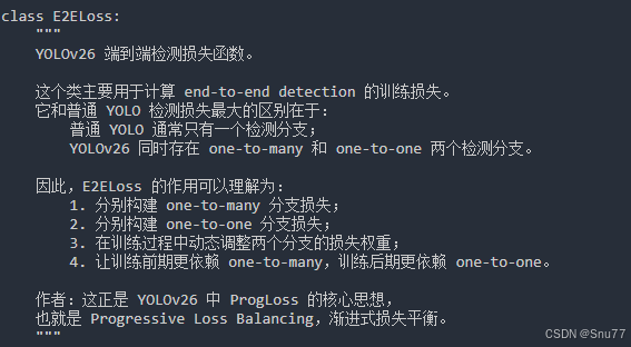
class E2ELoss:
    """
    YOLOv26 端到端检测损失函数。

    这个类主要用于计算 end-to-end detection 的训练损失。
    它和普通 YOLO 检测损失最大的区别在于:
        普通 YOLO 通常只有一个检测分支;
        YOLOv26 同时存在 one-to-many 和 one-to-one 两个检测分支。

    因此,E2ELoss 的作用可以理解为:
        1. 分别构建 one-to-many 分支损失;
        2. 分别构建 one-to-one 分支损失;
        3. 在训练过程中动态调整两个分支的损失权重;
        4. 让训练前期更依赖 one-to-many,训练后期更依赖 one-to-one。

    作者:这正是 YOLOv26 中 ProgLoss 的核心思想,
    也就是 Progressive Loss Balancing,渐进式损失平衡。
    """

    def __init__(self, model, loss_fn=v8DetectionLoss):
        """
        初始化 E2ELoss。

        Args:
            model:
                当前 YOLOv26 模型。

            loss_fn:
                基础检测损失函数,默认使用 v8DetectionLoss。

        需要注意:
            虽然这里默认叫 v8DetectionLoss,
            但在 YOLOv26 中它已经被用作基础检测损失计算模块。
            E2ELoss 会用它分别计算 one-to-many 和 one-to-one 两个分支的 loss。
        """

        # ============================================================
        # 1. one-to-many 分支损失
        # ============================================================

        # one2many 使用 tal_topk=10。
        #
        # tal_topk=10 表示在标签分配时,一个真实目标可以匹配多个候选正样本。
        # 这种方式更接近传统 YOLO 的密集监督方式。
        #
        # 我理解 one-to-many 分支的作用是:
        #     在训练前期提供更多正样本,
        #     让模型更容易学习目标位置和类别,
        #     提高训练稳定性和召回能力。
        self.one2many = loss_fn(model, tal_topk=10)

        # ============================================================
        # 2. one-to-one 分支损失
        # ============================================================

        # one2one 使用 tal_topk=7, tal_topk2=1。
        #
        # tal_topk=7:
        #     先在初步标签分配时选择一定数量的候选样本。
        #
        # tal_topk2=1:
        #     再进一步筛选,使一个目标最终更倾向于对应一个预测结果。
        #
        # 这和 YOLOv26 的端到端无 NMS 推理是一致的。
        # 因为推理阶段默认使用 one-to-one head,
        # 所以训练阶段也需要让 one-to-one 分支学习“一目标一预测”的模式。
        self.one2one = loss_fn(model, tal_topk=7, tal_topk2=1)

        # ============================================================
        # 3. 更新次数
        # ============================================================

        # updates 用于记录当前已经更新了多少次损失权重。
        #
        # 每调用一次 update(),
        # updates 就会加 1,
        # 然后根据 decay() 函数重新计算 one-to-many 和 one-to-one 的权重。
        self.updates = 0

        # ============================================================
        # 4. 两个分支损失权重之和
        # ============================================================

        # total 表示 one-to-many 和 one-to-one 两个分支的总权重。
        #
        # 后面始终保持:
        #     o2m + o2o = 1.0
        self.total = 1.0

        # ============================================================
        # 5. 初始损失权重
        # ============================================================

        # o2m 表示 one-to-many loss 的权重。
        #
        # 初始时设置为 0.8,
        # 说明训练前期更重视 one-to-many 分支。
        #
        # 这样做的原因是:
        #     one-to-many 分支正样本更多,
        #     训练信号更密集,
        #     有利于模型在早期稳定收敛。
        self.o2m = 0.8

        # o2o 表示 one-to-one loss 的权重。
        #
        # 因为 total=1.0,
        # 所以初始 o2o = 1.0 - 0.8 = 0.2。
        #
        # 也就是说训练初期:
        #     one-to-many 占 80%
        #     one-to-one 占 20%
        self.o2o = self.total - self.o2m

        # 保存 one-to-many 的初始权重。
        #
        # 后面的 decay() 函数需要知道初始 o2m 是多少,
        # 然后逐渐把它衰减到 final_o2m。
        self.o2m_copy = self.o2m

        # ============================================================
        # 6. 最终 one-to-many 权重
        # ============================================================

        # final_o2m 表示训练后期 one-to-many 分支最终保留的权重。
        #
        # 这里设置为 0.1,
        # 说明训练后期 one-to-many 分支不会完全消失,
        # 但它的重要性会大幅降低。
        #
        # 对应地,one-to-one 权重会逐渐增加到:
        #     o2o = 1.0 - 0.1 = 0.9
        self.final_o2m = 0.1

    def __call__(self, preds: Any, batch: dict[str, torch.Tensor]) -> tuple[torch.Tensor, torch.Tensor]:
        """
        计算 YOLOv26 端到端检测总损失。

        Args:
            preds:
                Detect 检测头输出结果。
                在 YOLOv26 end2end=True 时,preds 中包含:
                    preds["one2many"]
                    preds["one2one"]

            batch:
                当前 batch 的真实标签信息。

        Returns:
            total_loss:
                加权后的端到端总损失,用于反向传播。

            loss_info:
                用于日志显示的 loss 信息。
                这里返回的是 one-to-one 分支的 loss_detach。
        """

        # ============================================================
        # 1. 解析模型输出
        # ============================================================

        # parse_output 的作用是处理不同格式的 preds。
        #
        # 如果 preds 是 tuple:
        #     说明可能是 (最终预测结果, 原始预测字典)
        #     此时取 preds[1]。
        #
        # 如果 preds 本身就是 dict:
        #     直接返回。
        #
        # 在 YOLOv26 训练阶段,最终我们需要拿到:
        #     preds["one2many"]
        #     preds["one2one"]
        preds = self.one2many.parse_output(preds)

        # ============================================================
        # 2. 拆分两个检测分支
        # ============================================================

        # one2many:
        #     用于密集监督。
        #
        # one2one:
        #     用于对齐端到端无 NMS 推理。
        one2many, one2one = preds["one2many"], preds["one2one"]

        # ============================================================
        # 3. 计算 one-to-many 分支损失
        # ============================================================

        # 调用基础检测损失函数计算 one-to-many loss。
        #
        # loss_one2many[0]:
        #     用于反向传播的总损失。
        #
        # loss_one2many[1]:
        #     detach 后的 box/cls/dfl loss 信息,通常用于日志显示。
        loss_one2many = self.one2many.loss(one2many, batch)

        # ============================================================
        # 4. 计算 one-to-one 分支损失
        # ============================================================

        # 调用基础检测损失函数计算 one-to-one loss。
        #
        # one-to-one 分支的标签分配更严格,
        # 更接近最终推理阶段的输出形式。
        loss_one2one = self.one2one.loss(one2one, batch)

        # ============================================================
        # 5. ProgLoss:动态加权两个分支损失
        # ============================================================

        # 这里是 ProgLoss 的核心代码。
        #
        # 总损失不是简单相加:
        #     loss_one2many + loss_one2one
        #
        # 而是加权相加:
        #     o2m * loss_one2many + o2o * loss_one2one
        #
        # 训练初期:
        #     o2m = 0.8
        #     o2o = 0.2
        #
        # 训练后期:
        #     o2m -> 0.1
        #     o2o -> 0.9
        #
        # 也就是说:
        #     前期主要依赖 one-to-many 的密集监督;
        #     后期逐渐强化 one-to-one,使训练目标更接近无 NMS 推理。
        return loss_one2many[0] * self.o2m + loss_one2one[0] * self.o2o, loss_one2one[1]

    def update(self) -> None:
        """
        更新 one-to-many 和 one-to-one 两个分支的损失权重。

        这个函数需要在训练过程中被调用。
        如果训练循环中没有调用 update(),
        那么 o2m 和 o2o 会一直停留在初始值:
            o2m = 0.8
            o2o = 0.2

        只有持续调用 update(),
        才能真正实现 ProgLoss 的“渐进式损失平衡”。
        """

        # 更新次数加 1。
        self.updates += 1

        # 根据当前 updates 计算 one-to-many 的新权重。
        #
        # 随着训练进行,o2m 会从 0.8 逐渐衰减到 0.1。
        self.o2m = self.decay(self.updates)

        # one-to-one 的权重等于 total - o2m。
        #
        # 因为 total=1.0,
        # 所以随着 o2m 降低,o2o 会逐渐增大。
        #
        # max(..., 0) 是为了避免出现负数。
        self.o2o = max(self.total - self.o2m, 0)

    def decay(self, x) -> float:
        """
        计算 one-to-many 分支权重的衰减值。

        Args:
            x:
                当前更新次数,也就是 self.updates。

        Returns:
            当前 one-to-many 分支的权重 o2m。

        公式:
            o2m = max(1 - x / (epochs - 1), 0) * (init_o2m - final_o2m) + final_o2m

        其中:
            init_o2m = 0.8
            final_o2m = 0.1
        """

        # self.one2one.hyp.epochs 表示总训练 epoch 数。
        #
        # max(self.one2one.hyp.epochs - 1, 1)
        # 是为了避免 epochs=1 时除以 0。
        #
        # max(1 - x / ..., 0)
        # 表示随着训练推进,从 1 逐渐下降到 0。
        #
        # 整体效果:
        #     x=0 时,o2m 接近 0.8;
        #     x 接近 epochs 时,o2m 接近 0.1。
        return (
            max(1 - x / max(self.one2one.hyp.epochs - 1, 1), 0)
            * (self.o2m_copy - self.final_o2m)
            + self.final_o2m
        )
三、本文总结
到此本文的正式分享内容就结束了,在这里给大家推荐我的YOLOv26改进有效涨点专栏,本专栏目前为新开的平均质量分98分,后期我会根据各种最新的前沿顶会进行论文复现,也会对一些老的改进机制进行补充,目前本专栏免费阅读(暂时,大家尽早关注不迷路~),如果大家觉得本文帮助到你了,订阅本专栏,关注后续更多的更新~
专栏回顾:YOLOv26有效涨点专栏包含:Conv、注意力机制、主干/Backbone、损失函数、优化器、后处理等改进机制


AtomGit 是由开放原子开源基金会联合 CSDN 等生态伙伴共同推出的新一代开源与人工智能协作平台。平台坚持“开放、中立、公益”的理念,把代码托管、模型共享、数据集托管、智能体开发体验和算力服务整合在一起,为开发者提供从开发、训练到部署的一站式体验。
更多推荐


 8
8 0
0- 0


 已为社区贡献17条内容

所有评论(0)