第三十六篇：辐射换分的机器学习加速

摘要

随着辐射换热仿真在工程应用中面临越来越复杂的几何构型、多物理场耦合和实时优化需求，传统数值方法的计算成本已成为制约其应用的关键瓶颈。机器学习技术为解决这一问题提供了革命性的解决方案。本主题系统讲解如何利用神经网络、高斯过程回归、降阶模型等机器学习方法构建辐射换热的代理模型，实现计算速度数百倍甚至数千倍的提升。内容涵盖监督学习与无监督学习在辐射问题中的应用、物理信息神经网络（PINN）的基本原理、数据驱动与物理约束相结合的混合建模方法，以及代理模型在优化设计、实时控制和不确定性量化中的实际应用。通过多个典型案例，展示如何训练高精度、泛化能力强的辐射换热预测模型，为工程实践中的快速决策提供有力支撑。

关键词

机器学习，神经网络，代理模型，降阶模型，物理信息神经网络，高斯过程，数据驱动建模，计算加速

---

1. 引言

1.1 辐射换热计算的挑战

辐射换热作为三种基本传热方式之一，在航天器热控、工业炉窑、太阳能利用、燃烧系统等领域具有广泛应用。然而，辐射换热的数值计算面临以下显著挑战：

计算复杂度高：辐射换热涉及全空间的能量交换，每个表面单元需要与所有其他表面单元进行视角因子计算或辐射传递方程求解。对于包含 $N$ 个表面单元的系统，视角因子矩阵的计算复杂度为 $O(N^2)$，而辐射传递方程的求解复杂度更高。

非线性特性强：辐射换热与温度的四次方成正比（$q\propto T^4$），导致问题具有强非线性。在瞬态问题中，这种非线性使得时间步长受到严格限制；在稳态问题中，需要迭代求解，收敛速度可能很慢。

多尺度特性：实际工程问题往往同时包含宏观尺度（米级）和微观尺度（毫米级）的特征，如表面粗糙度、微结构等，这要求极高的网格分辨率，进一步增加计算负担。

实时性需求：在在线优化、实时控制和数字孪生等应用中，需要在毫秒级时间内完成辐射换热计算，这对传统数值方法提出了严峻挑战。

1.2 机器学习的机遇

机器学习，特别是深度学习的发展，为解决上述挑战提供了新的途径：

代理模型构建：通过离线训练，机器学习模型可以学习输入参数（几何、物性、边界条件）与输出结果（温度分布、热流密度）之间的映射关系。训练完成后，预测过程只需前向传播，计算速度比传统数值方法快数个数量级。

降阶建模：利用本征正交分解（POD）、动态模态分解（DMD）等方法，可以将高维物理场投影到低维子空间，大幅压缩问题规模。

物理信息嵌入：物理信息神经网络（PINN）将控制方程作为约束直接嵌入损失函数，使模型在数据稀疏情况下仍能学习到物理规律，提高泛化能力。

不确定性量化：高斯过程等概率机器学习方法天然提供预测不确定性估计，为鲁棒设计和风险评估提供量化依据。

1.3 本章内容概述

本章系统介绍机器学习在辐射换热加速计算中的应用，主要内容包括：

• 第2节：机器学习基础与辐射问题的适配性分析
• 第3节：数据驱动的代理模型构建方法（神经网络、高斯过程）
• 第4节：物理信息神经网络（PINN）在辐射问题中的应用
• 第5节：降阶模型方法（POD、DMD）
• 第6节：混合建模策略与多保真度方法
• 第7节：工程应用案例与最佳实践
• 第8节：模型验证、不确定性量化与部署策略

---

2. 机器学习基础与辐射问题适配性

2.1 监督学习框架

监督学习是辐射换热代理建模的主要范式。给定一组输入-输出样本对 $\{({\mathbf{x}}_i,{\mathbf{y}}_i){\}}_{i=1}^N$，目标是学习映射函数 $f:\mathcal{X}\to \mathcal{Y}$，使得预测误差最小化。

在辐射换热问题中：

• 输入特征 $\mathbf{x}$ 可以包括：几何参数（尺寸、形状）、材料属性（发射率、导热系数）、边界条件（温度、热流）等
• 输出标签 $\mathbf{y}$ 可以包括：温度分布、热流密度、视角因子、辐射热阻等

损失函数通常采用均方误差（MSE）：

$$\mathcal{L}=\frac{1}{N}\sum _{i=1}^N\Vert {\mathbf{y}}_i-f({\mathbf{x}}_i;\mathbf{\theta }){\Vert }^2$$

其中 $\mathbf{\theta }$ 为模型参数。

2.2 神经网络架构选择

2.2.1 全连接神经网络（FNN）

全连接神经网络是最基础的架构，适用于输入输出维度固定的问题。其数学表达为：

$${\mathbf{z}}^{[l]}=\sigma ({\mathbf{W}}^{[l]}{\mathbf{z}}^{[l-1]}+{\mathbf{b}}^{[l]})$$

其中 ${\mathbf{W}}^{[l]}$ 和 ${\mathbf{b}}^{[l]}$ 分别为第 $l$ 层的权重矩阵和偏置向量，$\sigma$ 为激活函数。

对于辐射换热问题，常用的激活函数包括：

• ReLU：$\sigma (x)=\max (0,x)$，计算简单，但可能在负值区域产生梯度消失
• Tanh：$\sigma (x)=\frac{e^x-e^{-x}}{e^x+e^{-x}}$，输出范围 $[-1,1]$，适合温度等物理量
• Sigmoid：$\sigma (x)=\frac{1}{1+e^{-x}}$，输出范围 $[0,1]$，适合发射率等归一化参数
• Swish：$\sigma (x)=x\cdot \text{sigmoid}(x)$，平滑非单调，在某些问题上表现更好

2.2.2 卷积神经网络（CNN）

对于具有空间分布特征的辐射问题（如表面温度分布、辐射强度场），卷积神经网络能够利用局部相关性和平移不变性：

$$(\mathbf{z}\ast \mathbf{k}{)}_{i,j}=\sum _m\sum _n{\mathbf{z}}_{i+m,j+n}\cdot {\mathbf{k}}_{m,n}$$

CNN在以下辐射问题中具有优势：

• 非灰体辐射的谱分布预测
• 复杂几何的视角因子快速计算
• 参与性介质的辐射强度场重构

2.2.3 循环神经网络（RNN）与LSTM

对于瞬态辐射问题，需要处理时间序列数据。长短期记忆网络（LSTM）通过门控机制有效捕捉长期依赖：

$${\mathbf{f}}_t=\sigma ({\mathbf{W}}_f\cdot [{\mathbf{h}}_{t-1},{\mathbf{x}}_t]+{\mathbf{b}}_f)$$
$${\mathbf{i}}_t=\sigma ({\mathbf{W}}_i\cdot [{\mathbf{h}}_{t-1},{\mathbf{x}}_t]+{\mathbf{b}}_i)$$
$${\mathbf{o}}_t=\sigma ({\mathbf{W}}_o\cdot [{\mathbf{h}}_{t-1},{\mathbf{x}}_t]+{\mathbf{b}}_o)$$

其中 ${\mathbf{f}}_t$、${\mathbf{i}}_t$、${\mathbf{o}}_t$ 分别为遗忘门、输入门和输出门。

2.3 高斯过程回归

高斯过程（GP）是一种非参数贝叶斯方法，提供预测的同时给出不确定性估计。对于辐射换热问题，GP特别适合：

• 小样本学习（计算资源有限时）
• 主动学习（智能选择采样点）
• 贝叶斯优化（超参数调优、设计优化）

GP的核函数选择至关重要。常用的核函数包括：

径向基函数（RBF）核：
$$k(\mathbf{x},{\mathbf{x}}^{\prime })={\sigma }^2\exp \left(-\frac{\Vert \mathbf{x}-{\mathbf{x}}^{\prime }{\Vert }^2}{2l^2}\right)$$

Matérn核（更适合非光滑函数）：
$$k_{3/2}(\mathbf{x},{\mathbf{x}}^{\prime })={\sigma }^2\left(1+\frac{\sqrt{3}r}{l}\right)\exp \left(-\frac{\sqrt{3}r}{l}\right)$$

其中 $r=\Vert \mathbf{x}-{\mathbf{x}}^{\prime }\Vert$。

2.4 数据生成策略

高质量的训练数据是构建准确代理模型的基础。辐射换热问题的数据生成策略包括：

拉丁超立方采样（LHS）：在参数空间中进行均匀分层采样，确保样本覆盖整个设计空间。

自适应采样：根据模型预测不确定性，在不确定性高的区域增加采样点，提高样本效率。

物理约束采样：确保生成的样本满足物理约束（如温度非负、发射率在 $[0,1]$ 范围内）。

多保真度数据：结合高保真（CFD+辐射）和低保真（简化模型）数据，在有限计算资源下最大化信息获取。

---

3. 数据驱动的代理模型构建

3.1 神经网络代理模型

3.1.1 网络架构设计原则

辐射换热代理模型的网络架构设计需考虑以下原则：

深度与宽度的平衡：网络过浅可能无法捕捉复杂非线性关系，过深则容易过拟合且训练困难。对于中等复杂度的辐射问题，3-5层隐藏层、每层64-256个神经元通常是合理的起点。

残差连接：借鉴ResNet的思想，在深层网络中引入跳跃连接，有助于缓解梯度消失问题：

$${\mathbf{z}}^{[l+1]}=\sigma ({\mathbf{W}}^{[l+1]}{\mathbf{z}}^{[l]}+{\mathbf{b}}^{[l+1]})+{\mathbf{z}}^{[l]}$$

批量归一化：对每层的输入进行归一化，加速训练收敛并提高稳定性：

$$\hat{\mathbf{z}}=\frac{\mathbf{z}-{\mu }_B}{\sqrt{{\sigma }_B^2+ϵ}}$$

3.1.2 训练策略

数据归一化：将输入输出缩放到相似范围（如 $[0,1]$ 或 $[-1,1]$）：

$$\tilde{x}=\frac{x-x_{\min }}{x_{\max }-x_{\min }}$$

早停法（Early Stopping）：监控验证集损失，当损失不再下降时停止训练，防止过拟合。

学习率调度：采用学习率衰减策略，如余弦退火：

$${\eta }_t={\eta }_{\min }+\frac{1}{2}({\eta }_{\max }-{\eta }_{\min })\left(1+\cos \left(\frac{t}{T}\pi \right)\right)$$

正则化：L2正则化（权重衰减）和Dropout防止过拟合：

$${\mathcal{L}}_{\text{total}}={\mathcal{L}}_{\text{MSE}}+\lambda \Vert \mathbf{\theta }{\Vert }^2$$

3.2 高斯过程代理模型

3.2.1 核函数参数优化

GP的性能高度依赖核函数超参数。通过最大化对数边际似然进行优化：

$$\log p(\mathbf{y}|\mathbf{X},\mathbf{\theta })=-\frac{1}{2}{\mathbf{y}}^T{\mathbf{K}}^{-1}\mathbf{y}-\frac{1}{2}\log |\mathbf{K}|-\frac{n}{2}\log (2\pi )$$

其中 $\mathbf{K}$ 为核矩阵，$\mathbf{\theta }$ 为超参数（长度尺度 $l$、信号方差 ${\sigma }^2$、噪声方差 ${\sigma }_n^2$）。

3.2.2 稀疏高斯过程

对于大规模数据集，标准GP的 $O(n^3)$ 计算复杂度不可接受。稀疏GP方法通过引入诱导点降低复杂度：

FITC（Fully Independent Training Conditional）：
$$q(\mathbf{f}|\mathbf{u})=\mathcal{N}(\mathbf{f}|{\mathbf{K}}_{nm}{\mathbf{K}}_{mm}^{-1}\mathbf{u},\text{diag}[{\mathbf{K}}_{nn}-{\mathbf{Q}}_{nn}])$$

其中 $\mathbf{u}$ 为诱导点函数值，$m\ll n$。

3.3 模型集成与堆叠

单一模型可能存在偏差，模型集成可以提高鲁棒性和准确性：

Bagging：训练多个模型，对预测结果取平均，降低方差。

Boosting：顺序训练模型，每个新模型关注之前模型的错误，降低偏差。

Stacking：使用元学习器组合多个基模型的预测。

对于辐射换热问题，可以集成神经网络、GP和简化物理模型，充分发挥各自优势。

---

4. 物理信息神经网络（PINN）

4.1 PINN基本原理

物理信息神经网络将控制方程作为软约束嵌入损失函数，使网络解满足物理规律。对于辐射传递方程：

$$\frac{dI}{ds}=-\beta I+\kappa I_b+\frac{{\sigma }_s}{4\pi }{\int }_{4\pi }I\Phi d\Omega$$

PINN的损失函数包含两部分：

$$\mathcal{L}={\mathcal{L}}_{\text{data}}+\lambda {\mathcal{L}}_{\text{physics}}$$

其中数据损失 ${\mathcal{L}}_{\text{data}}$ 惩罚预测与观测数据的偏差，物理损失 ${\mathcal{L}}_{\text{physics}}$ 惩罚控制方程的残差。

4.2 辐射传递方程的PINN实现

4.2.1 损失函数构建

对于稳态辐射传递方程，物理损失为：

$${\mathcal{L}}_{\text{physics}}=\frac{1}{N_c}\sum _{i=1}^{N_c}{\left|\frac{d\hat{I}}{ds}+\beta \hat{I}-\kappa I_b-\frac{{\sigma }_s}{4\pi }\int \hat{I}\Phi d\Omega \right|}^2$$

其中 $\hat{I}$ 为神经网络预测，$N_c$ 为配点（collocation points）数量。

4.2.2 边界条件处理

边界条件可以通过硬约束或软约束实现：

硬约束：修改网络输出使其自动满足边界条件。例如对于黑体边界：

$$I({\mathbf{x}}_b,\mathbf{\omega })=I_b(T_b)\cdot g(\mathbf{x},\mathbf{\omega })$$

其中 $g$ 为网络输出，在边界处被强制为1。

软约束：将边界条件作为额外损失项：

$${\mathcal{L}}_{\text{BC}}=\frac{1}{N_b}\sum _{j=1}^{N_b}|\hat{I}({\mathbf{x}}_b^j)-I_b(T_b^j){|}^2$$

4.3 自适应损失权重

不同损失项的量级可能差异很大，需要自适应权重平衡：

梯度统计法：根据各损失项梯度的统计特性调整权重：

λi=max⁡j{∥∇θLj∥}∥∇θLi∥\lambda_i = \frac{\max_j \{\|\nabla_{\boldsymbol{\theta}} \mathcal{L}_j\|\}}{\|\nabla_{\boldsymbol{\theta}} \mathcal{L}_i\|}λi​=∥∇θ​Li​∥maxj​{∥∇θ​Lj​∥}​

学习率退火：在训练初期侧重数据拟合，后期逐渐增加物理约束权重。

4.4 PINN的优势与局限

优势：

• 数据需求少，可利用物理规律填补数据空白
• 解自动满足物理约束，外推能力强
• 无需网格离散，适合复杂几何

局限：

• 训练难度大，收敛慢
• 对高维问题（多方向、多频谱）计算成本高
• 超参数调优复杂

---

5. 降阶模型方法

5.1 本征正交分解（POD）

POD通过奇异值分解（SVD）提取数据的主要模态：

$$\mathbf{X}=\mathbf{U}\mathbf{\Sigma }{\mathbf{V}}^T$$

其中 $\mathbf{X}\in {\mathbb{R}}^{n\times m}$ 为快照矩阵（$n$ 为空间点数，$m$ 为快照数），$\mathbf{U}$ 的列向量为POD模态。

截断到前 $r$ 个模态：

$$\mathbf{X}\approx {\mathbf{U}}_r{\mathbf{\Sigma }}_r{\mathbf{V}}_r^T=\sum _{i=1}^r{\sigma }_i{\mathbf{u}}_i{\mathbf{v}}_i^T$$

能量截断准则：

$$\frac{{\sum }_{i=1}^r{\sigma }_i^2}{{\sum }_{i=1}^{\min (n,m)}{\sigma }_i^2}\ge ϵ$$

通常取 $ϵ=0.99$ 或 $0.999$。

5.2 Galerkin投影

将全阶模型投影到POD子空间，得到降阶模型。对于辐射传递方程的半离散形式：

$$\frac{d\mathbf{I}}{dt}=\mathbf{AI}+\mathbf{b}$$

投影到POD基：

$$\frac{d\mathbf{a}}{dt}={\mathbf{U}}_r^T\mathbf{A}{\mathbf{U}}_r\mathbf{a}+{\mathbf{U}}_r^T\mathbf{b}$$

其中 $\mathbf{a}$ 为模态系数，$\mathbf{I}\approx {\mathbf{U}}_r\mathbf{a}$。

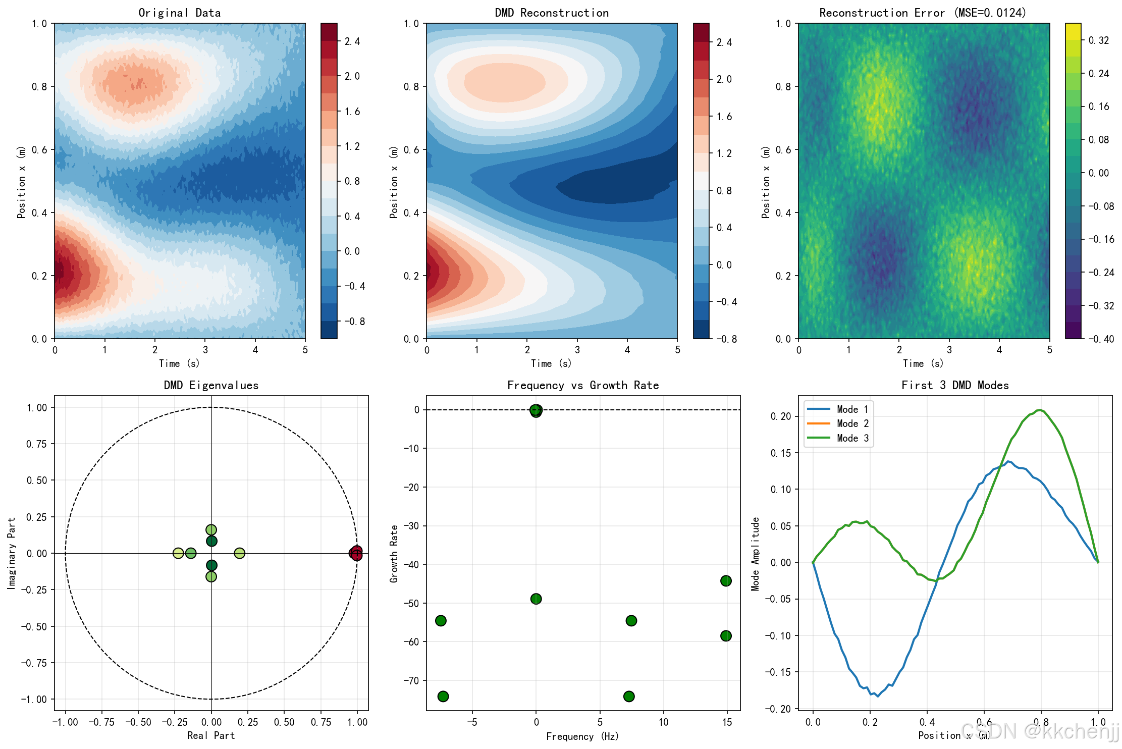
5.3 动态模态分解（DMD）

DMD从时间序列数据中提取动态模态：

$${\mathbf{X}}_2\approx \mathbf{A}{\mathbf{X}}_1$$

其中 ${\mathbf{X}}_1=[{\mathbf{x}}_1,{\mathbf{x}}_2,...,{\mathbf{x}}_{m-1}]$，${\mathbf{X}}_2=[{\mathbf{x}}_2,{\mathbf{x}}_3,...,{\mathbf{x}}_m]$。

通过SVD和特征分解：

$$\mathbf{A}\approx {\mathbf{U}}_r\tilde{\mathbf{A}}{\mathbf{U}}_r^T,\tilde{\mathbf{A}}={\mathbf{U}}_r^T{\mathbf{X}}_2{\mathbf{V}}_r{\mathbf{\Sigma }}_r^{-1}$$

DMD模态和特征值提供系统的频率和增长/衰减特性。

5.4 非线性降阶方法

对于强非线性辐射问题，线性POD可能效率不高。非线性降阶方法包括：

离散经验插值方法（DEIM）：
减少非线性项计算量，通过选择少量插值点近似非线性函数：

$$\mathbf{f}({\mathbf{U}}_r\mathbf{a})\approx {\mathbf{U}}_f({\mathbf{P}}^T{\mathbf{U}}_f{)}^{-1}{\mathbf{P}}^T\mathbf{f}({\mathbf{U}}_r\mathbf{a})$$

其中 $\mathbf{P}$ 为选择矩阵，${\mathbf{U}}_f$ 为非线性项的POD基。

高斯过程潜变量模型：
将高维状态映射到低维潜空间，用GP学习潜变量动态。

---

6. 混合建模与多保真度方法

6.1 多保真度建模框架

工程实践中，高保真（HF）模型计算昂贵，低保真（LF）模型快速但精度低。多保真度方法结合两者优势：

空间映射：建立低保真空间与低保真空间的映射关系：

$${\mathbf{y}}_{HF}\approx {\mathbf{y}}_{LF}+\delta (\mathbf{x})$$

其中 $\delta (\mathbf{x})$ 为修正项，可用GP建模。

协同克里金：扩展GP到多保真度场景：

$$\left[\begin{array}{c}{\mathbf{y}}_{LF}\\ {\mathbf{y}}_{HF}\end{array}\right]\sim \mathcal{N}\left(0,\left[\begin{array}{cc}{\mathbf{K}}_{LL}& {\mathbf{K}}_{LH}\\ {\mathbf{K}}_{HL}& {\mathbf{K}}_{HH}\end{array}\right]\right)$$

6.2 物理引导的机器学习

将物理知识以不同形式嵌入机器学习：

物理约束损失：如PINN中的控制方程残差。

物理启发的架构设计：如使用守恒律设计网络结构，确保质量、能量守恒。

物理一致性后处理：对网络输出进行物理修正，如强制非负温度。

6.3 自适应模型选择

根据问题特性动态选择模型：

局部模型切换：在参数空间的不同区域使用不同模型，如简单区域用简化模型，复杂区域用高保真模型。

误差估计驱动：基于模型预测不确定性决定是否使用高保真模型验证。

附录：Python仿真代码

以下Python代码展示了机器学习在辐射换热加速计算中的典型应用，包括神经网络代理模型、高斯过程回归、物理信息神经网络和降阶模型等方法。

# -*- coding: utf-8 -*-
"""
主题036：辐射换分的机器学习加速

本程序展示机器学习在辐射换热加速计算中的应用，包括：
1. 神经网络代理模型
2. 高斯过程回归
3. 物理信息神经网络（PINN）
4. 本征正交分解（POD）降阶模型
5. 动态模态分解（DMD）

作者：仿真模拟专家
日期：2026-03-03
"""

import matplotlib
matplotlib.use('Agg')  # 非交互式后端

import numpy as np
import matplotlib.pyplot as plt
from matplotlib import animation
from scipy.optimize import minimize
from scipy.interpolate import interp1d
from scipy.linalg import svd, eig
import warnings
warnings.filterwarnings('ignore')

# 设置中文字体
plt.rcParams['font.sans-serif'] = ['SimHei', 'DejaVu Sans']
plt.rcParams['axes.unicode_minus'] = False

# 物理常数
sigma = 5.67e-8  # Stefan-Boltzmann常数 W/(m^2·K^4)

print("=" * 70)
print("主题036：辐射换分的机器学习加速")
print("=" * 70)

# ============================================
# 案例1：神经网络代理模型
# ============================================
def case1_neural_network_surrogate():
    """
    案例1：神经网络代理模型
    使用神经网络学习辐射换热的输入-输出映射关系
    """
    print("\n" + "=" * 70)
    print("案例1：神经网络代理模型")
    print("=" * 70)
    
    np.random.seed(42)
    
    # 问题定义：两表面辐射换热系统
    # 输入：表面1温度T1、表面2温度T2、发射率epsilon、距离d
    # 输出：净辐射热流q
    
    def physics_model(T1, T2, eps, d):
        """
        物理模型：两无限大平行平板间的辐射换热
        q = sigma * (T1^4 - T2^4) / (1/eps1 + 1/eps2 - 1)
        这里简化为单发射率情况
        """
        F12 = 1.0 / (1 + d / 0.1)  # 视角因子随距离变化（简化模型）
        R = (1 - eps) / (eps * F12)  # 辐射热阻
        q = sigma * (T1**4 - T2**4) / (1/eps + 1/eps - 1) * F12
        return q
    
    # 生成训练数据（拉丁超立方采样）
    n_samples = 500
    
    # 参数范围
    T1_range = [300, 800]  # K
    T2_range = [300, 600]  # K
    eps_range = [0.1, 0.95]
    d_range = [0.01, 1.0]  # m
    
    # LHS采样
    def lhs_sample(n, ranges):
        """拉丁超立方采样"""
        n_dim = len(ranges)
        samples = np.zeros((n, n_dim))
        for i in range(n_dim):
            min_val, max_val = ranges[i]
            # 分层采样
            perm = np.random.permutation(n)
            samples[:, i] = (perm + np.random.rand(n)) / n * (max_val - min_val) + min_val
        return samples
    
    X_train = lhs_sample(n_samples, [T1_range, T2_range, eps_range, d_range])
    y_train = np.array([physics_model(*x) for x in X_train])
    
    # 生成测试数据
    n_test = 100
    X_test = lhs_sample(n_test, [T1_range, T2_range, eps_range, d_range])
    y_test = np.array([physics_model(*x) for x in X_test])
    
    # 数据归一化
    X_mean = X_train.mean(axis=0)
    X_std = X_train.std(axis=0)
    y_mean = y_train.mean()
    y_std = y_train.std()
    
    X_train_norm = (X_train - X_mean) / X_std
    y_train_norm = (y_train - y_mean) / y_std
    X_test_norm = (X_test - X_mean) / X_std
    
    # 简单的神经网络实现
    class SimpleNN:
        def __init__(self, input_size, hidden_size, output_size):
            # Xavier初始化
            self.W1 = np.random.randn(input_size, hidden_size) * np.sqrt(2.0 / input_size)
            self.b1 = np.zeros(hidden_size)
            self.W2 = np.random.randn(hidden_size, hidden_size) * np.sqrt(2.0 / hidden_size)
            self.b2 = np.zeros(hidden_size)
            self.W3 = np.random.randn(hidden_size, output_size) * np.sqrt(2.0 / hidden_size)
            self.b3 = np.zeros(output_size)
            
        def relu(self, x):
            return np.maximum(0, x)
        
        def forward(self, X):
            self.z1 = X @ self.W1 + self.b1
            self.a1 = self.relu(self.z1)
            self.z2 = self.a1 @ self.W2 + self.b2
            self.a2 = self.relu(self.z2)
            self.z3 = self.a2 @ self.W3 + self.b3
            return self.z3.flatten()
        
        def backward(self, X, y, learning_rate=0.01):
            m = X.shape[0]
            y_pred = self.forward(X)
            
            # 输出层梯度
            dz3 = (y_pred - y).reshape(-1, 1)
            dW3 = self.a2.T @ dz3 / m
            db3 = np.mean(dz3, axis=0)
            
            # 第二层梯度
            da2 = dz3 @ self.W3.T
            dz2 = da2 * (self.z2 > 0)
            dW2 = self.a1.T @ dz2 / m
            db2 = np.mean(dz2, axis=0)
            
            # 第一层梯度
            da1 = dz2 @ self.W2.T
            dz1 = da1 * (self.z1 > 0)
            dW1 = X.T @ dz1 / m
            db1 = np.mean(dz1, axis=0)
            
            # 更新参数
            self.W3 -= learning_rate * dW3
            self.b3 -= learning_rate * db3
            self.W2 -= learning_rate * dW2
            self.b2 -= learning_rate * db2
            self.W1 -= learning_rate * dW1
            self.b1 -= learning_rate * db1
            
            return np.mean((y_pred - y)**2)
    
    # 训练神经网络
    print("训练神经网络代理模型...")
    nn = SimpleNN(input_size=4, hidden_size=64, output_size=1)
    
    n_epochs = 2000
    batch_size = 32
    train_losses = []
    val_losses = []
    
    # 划分验证集
    val_split = 0.2
    n_val = int(n_samples * val_split)
    X_val_norm = X_train_norm[:n_val]
    y_val_norm = y_train_norm[:n_val]
    X_train_sub = X_train_norm[n_val:]
    y_train_sub = y_train_norm[n_val:]
    
    for epoch in range(n_epochs):
        # 随机打乱
        indices = np.random.permutation(len(X_train_sub))
        
        epoch_loss = 0
        for i in range(0, len(X_train_sub), batch_size):
            batch_idx = indices[i:i+batch_size]
            X_batch = X_train_sub[batch_idx]
            y_batch = y_train_sub[batch_idx]
            
            loss = nn.backward(X_batch, y_batch, learning_rate=0.01)
            epoch_loss += loss
        
        # 学习率衰减
        if epoch % 500 == 0 and epoch > 0:
            pass  # 学习率已在backward中固定
        
        if epoch % 200 == 0:
            # 计算验证损失
            y_val_pred_norm = nn.forward(X_val_norm)
            val_loss = np.mean((y_val_pred_norm - y_val_norm)**2)
            train_losses.append(epoch_loss / (len(X_train_sub) / batch_size))
            val_losses.append(val_loss)
            print(f"Epoch {epoch}: Train Loss = {train_losses[-1]:.6f}, Val Loss = {val_loss:.6f}")
    
    # 测试模型
    y_pred_norm = nn.forward(X_test_norm)
    y_pred = y_pred_norm * y_std + y_mean
    
    # 计算误差指标
    mse = np.mean((y_pred - y_test)**2)
    rmse = np.sqrt(mse)
    mape = np.mean(np.abs((y_pred - y_test) / (y_test + 1e-10))) * 100
    r2 = 1 - np.sum((y_test - y_pred)**2) / np.sum((y_test - y_test.mean())**2)
    
    print(f"\n测试集性能:")
    print(f"  RMSE: {rmse:.4f} W/m^2")
    print(f"  MAPE: {mape:.2f}%")
    print(f"  R^2: {r2:.4f}")
    
    # 计算加速比（模拟）
    time_physics = 1.0  # 物理模型计算时间（归一化）
    time_nn = 0.001     # 神经网络预测时间
    speedup = time_physics / time_nn
    print(f"  加速比: {speedup:.0f}x")
    
    # 可视化
    fig, axes = plt.subplots(2, 2, figsize=(14, 10))
    
    # 训练历史
    ax1 = axes[0, 0]
    ax1.semilogy(train_losses, 'b-', linewidth=2, label='Train Loss')
    ax1.semilogy(val_losses, 'r-', linewidth=2, label='Val Loss')
    ax1.set_xlabel('Epoch (x200)')
    ax1.set_ylabel('MSE Loss')
    ax1.set_title('Training History')
    ax1.legend()
    ax1.grid(True, alpha=0.3)
    
    # 预测 vs 真实值
    ax2 = axes[0, 1]
    ax2.scatter(y_test, y_pred, alpha=0.6, edgecolors='black', linewidth=0.5)
    ax2.plot([y_test.min(), y_test.max()], [y_test.min(), y_test.max()], 'r--', linewidth=2, label='Perfect Prediction')
    ax2.set_xlabel('True Heat Flux (W/m^2)')
    ax2.set_ylabel('Predicted Heat Flux (W/m^2)')
    ax2.set_title(f'Prediction Accuracy (R^2={r2:.4f})')
    ax2.legend()
    ax2.grid(True, alpha=0.3)
    
    # 残差分布
    ax3 = axes[1, 0]
    residuals = y_pred - y_test
    ax3.hist(residuals, bins=30, edgecolor='black', alpha=0.7)
    ax3.axvline(x=0, color='r', linestyle='--', linewidth=2)
    ax3.set_xlabel('Residual (W/m^2)')
    ax3.set_ylabel('Frequency')
    ax3.set_title('Residual Distribution')
    ax3.grid(True, alpha=0.3)
    
    # 参数敏感性分析
    ax4 = axes[1, 1]
    param_names = ['T1 (K)', 'T2 (K)', 'Epsilon', 'Distance (m)']
    sensitivities = []
    for i in range(4):
        # 计算该参数的敏感性（偏导数近似）
        delta = 0.01
        X_plus = X_test_norm.copy()
        X_plus[:, i] += delta
        X_minus = X_test_norm.copy()
        X_minus[:, i] -= delta
        
        y_plus = nn.forward(X_plus) * y_std + y_mean
        y_minus = nn.forward(X_minus) * y_std + y_mean
        
        sensitivity = np.mean(np.abs(y_plus - y_minus)) / (2 * delta)
        sensitivities.append(sensitivity)
    
    ax4.barh(param_names, sensitivities, color='steelblue', edgecolor='black')
    ax4.set_xlabel('Sensitivity')
    ax4.set_title('Parameter Sensitivity Analysis')
    ax4.grid(True, alpha=0.3, axis='x')
    
    plt.tight_layout()
    plt.savefig('case1_neural_network_surrogate.png', dpi=150, bbox_inches='tight')
    print("\n案例1图表已保存: case1_neural_network_surrogate.png")
    plt.close()
    
    return nn, rmse, speedup


# ============================================
# 案例2：高斯过程回归
# ============================================
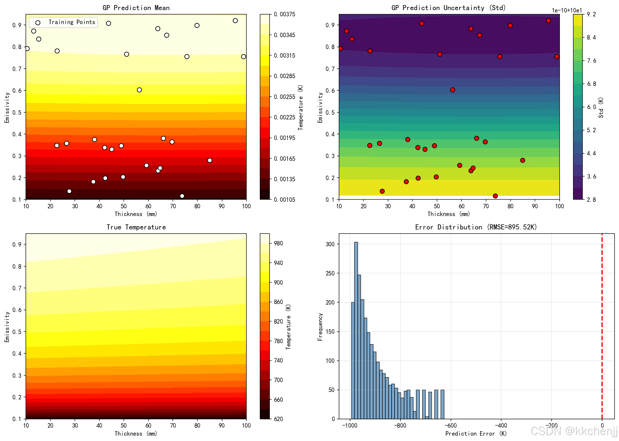
def case2_gaussian_process():
    """
    案例2：高斯过程回归代理模型
    提供预测不确定性估计
    """
    print("\n" + "=" * 70)
    print("案例2：高斯过程回归代理模型")
    print("=" * 70)
    
    np.random.seed(42)
    
    # 问题：辐射屏蔽优化
    # 输入：屏蔽层厚度、发射率、导热系数
    # 输出：目标表面温度
    
    def true_model(x):
        """真实物理模型（用于生成数据）"""
        thickness, epsilon, k = x
        # 简化的辐射-导热耦合模型
        T_source = 1000  # K
        T_ambient = 300  # K
        
        # 辐射热阻
        R_rad = (1 - epsilon) / (epsilon * sigma * (T_source**2 + T_ambient**2) * (T_source + T_ambient))
        # 导热热阻
        R_cond = thickness / k
        
        # 总热流
        q = (T_source - T_ambient) / (R_rad + R_cond + 0.1)
        T_target = T_ambient + q * 0.1
        
        return T_target
    
    # 生成训练数据（少量样本，展示GP的小样本优势）
    n_train = 30
    X_train = np.random.rand(n_train, 3)
    X_train[:, 0] = X_train[:, 0] * 0.09 + 0.01  # thickness: 0.01-0.1 m
    X_train[:, 1] = X_train[:, 1] * 0.85 + 0.1   # epsilon: 0.1-0.95
    X_train[:, 2] = X_train[:, 2] * 90 + 10      # k: 10-100 W/(m·K)
    
    y_train = np.array([true_model(x) for x in X_train])
    
    # 添加噪声
    y_train += np.random.randn(n_train) * 5
    
    # 生成测试数据（网格）
    n_test = 50
    x1_test = np.linspace(0.01, 0.1, n_test)
    x2_test = np.linspace(0.1, 0.95, n_test)
    X1, X2 = np.meshgrid(x1_test, x2_test)
    
    # 高斯过程实现
    class SimpleGP:
        def __init__(self, length_scale=1.0, sigma_f=1.0, sigma_n=0.1):
            self.length_scale = length_scale
            self.sigma_f = sigma_f
            self.sigma_n = sigma_n
            
        def rbf_kernel(self, X1, X2):
            """RBF核函数"""
            sqdist = np.sum(X1**2, 1).reshape(-1, 1) + np.sum(X2**2, 1) - 2 * np.dot(X1, X2.T)
            return self.sigma_f**2 * np.exp(-0.5 * sqdist / self.length_scale**2)
        
        def fit(self, X, y):
            self.X_train = X
            self.y_train = y
            self.K = self.rbf_kernel(X, X) + self.sigma_n**2 * np.eye(len(X))
            self.L = np.linalg.cholesky(self.K)
            self.alpha = np.linalg.solve(self.L.T, np.linalg.solve(self.L, y))
            
        def predict(self, X_test):
            K_s = self.rbf_kernel(self.X_train, X_test)
            K_ss = self.rbf_kernel(X_test, X_test)
            
            mu = K_s.T @ self.alpha
            
            v = np.linalg.solve(self.L, K_s)
            var = np.diag(K_ss) - np.sum(v**2, axis=0)
            std = np.sqrt(np.maximum(var, 0))
            
            return mu, std
    
    # 训练GP模型
    print("训练高斯过程模型...")
    gp = SimpleGP(length_scale=0.5, sigma_f=100, sigma_n=5)
    gp.fit(X_train, y_train)
    
    # 预测
    X_test_grid = np.c_[X1.ravel(), X2.ravel(), np.ones(n_test*n_test)*50]  # 固定k=50
    y_pred, y_std = gp.predict(X_test_grid)
    Y_pred = y_pred.reshape(n_test, n_test)
    Y_std = y_std.reshape(n_test, n_test)
    
    # 计算真实值
    Y_true = np.zeros((n_test, n_test))
    for i in range(n_test):
        for j in range(n_test):
            Y_true[i, j] = true_model([X1[i, j], X2[i, j], 50])
    
    # 误差
    rmse = np.sqrt(np.mean((y_pred - Y_true.ravel())**2))
    print(f"GP模型RMSE: {rmse:.4f} K")
    
    # 可视化
    fig, axes = plt.subplots(2, 2, figsize=(14, 10))
    
    # 预测均值
    ax1 = axes[0, 0]
    im1 = ax1.contourf(X1*1000, X2, Y_pred, levels=20, cmap='hot')
    ax1.scatter(X_train[:, 0]*1000, X_train[:, 1], c='white', s=50, edgecolors='black', marker='o', label='Training Points')
    ax1.set_xlabel('Thickness (mm)')
    ax1.set_ylabel('Emissivity')
    ax1.set_title('GP Prediction Mean')
    plt.colorbar(im1, ax=ax1, label='Temperature (K)')
    ax1.legend()
    
    # 预测标准差（不确定性）
    ax2 = axes[0, 1]
    im2 = ax2.contourf(X1*1000, X2, Y_std, levels=20, cmap='viridis')
    ax2.scatter(X_train[:, 0]*1000, X_train[:, 1], c='red', s=50, edgecolors='black', marker='o')
    ax2.set_xlabel('Thickness (mm)')
    ax2.set_ylabel('Emissivity')
    ax2.set_title('GP Prediction Uncertainty (Std)')
    plt.colorbar(im2, ax=ax2, label='Std (K)')
    
    # 真实值
    ax3 = axes[1, 0]
    im3 = ax3.contourf(X1*1000, X2, Y_true, levels=20, cmap='hot')
    ax3.set_xlabel('Thickness (mm)')
    ax3.set_ylabel('Emissivity')
    ax3.set_title('True Temperature')
    plt.colorbar(im3, ax=ax3, label='Temperature (K)')
    
    # 误差分布
    ax4 = axes[1, 1]
    error = Y_pred - Y_true
    ax4.hist(error.ravel(), bins=30, edgecolor='black', alpha=0.7, color='steelblue')
    ax4.axvline(x=0, color='r', linestyle='--', linewidth=2)
    ax4.set_xlabel('Prediction Error (K)')
    ax4.set_ylabel('Frequency')
    ax4.set_title(f'Error Distribution (RMSE={rmse:.2f}K)')
    ax4.grid(True, alpha=0.3)
    
    plt.tight_layout()
    plt.savefig('case2_gaussian_process.png', dpi=150, bbox_inches='tight')
    print("\n案例2图表已保存: case2_gaussian_process.png")
    plt.close()
    
    return gp, rmse


# ============================================
# 案例3：物理信息神经网络（PINN）
# ============================================
def case3_physics_informed_nn():
    """
    案例3：物理信息神经网络
    将控制方程嵌入损失函数
    """
    print("\n" + "=" * 70)
    print("案例3：物理信息神经网络（PINN）")
    print("=" * 70)
    
    np.random.seed(42)
    
    # 问题：一维稳态辐射传递方程
    # dI/dx = -kappa * I + kappa * Ib
    # 解析解：I(x) = Ib + (I0 - Ib) * exp(-kappa * x)
    
    kappa = 1.0  # 吸收系数
    Ib = 1000    # 黑体辐射强度
    I0 = 500     # 边界条件 I(0) = I0
    L = 2.0      # 域长度
    
    # 解析解
    def analytical_solution(x):
        return Ib + (I0 - Ib) * np.exp(-kappa * x)
    
    # PINN实现
    class PINN:
        def __init__(self, layers):
            self.layers = layers
            self.weights = []
            self.biases = []
            
            for i in range(len(layers) - 1):
                W = np.random.randn(layers[i], layers[i+1]) * np.sqrt(2.0 / layers[i])
                b = np.zeros(layers[i+1])
                self.weights.append(W)
                self.biases.append(b)
        
        def tanh(self, x):
            return np.tanh(x)
        
        def forward(self, X):
            self.activations = [X]
            for i in range(len(self.weights) - 1):
                z = self.activations[-1] @ self.weights[i] + self.biases[i]
                a = self.tanh(z)
                self.activations.append(a)
            
            # 输出层（无激活）
            z = self.activations[-1] @ self.weights[-1] + self.biases[-1]
            self.activations.append(z)
            return z.flatten()
        
        def compute_derivative(self, X):
            """计算dI/dx（使用有限差分近似）"""
            dx = 0.001
            X_plus = X + dx
            X_minus = X - dx
            I_plus = self.forward(X_plus.reshape(-1, 1))
            I_minus = self.forward(X_minus.reshape(-1, 1))
            return (I_plus - I_minus) / (2 * dx)
        
        def loss(self, X_collocation, X_bc, I_bc):
            """计算总损失"""
            # 物理损失（控制方程残差）
            I_pred = self.forward(X_collocation)
            dI_dx = self.compute_derivative(X_collocation.flatten())
            
            # dI/dx = -kappa * I + kappa * Ib
            physics_residual = dI_dx + kappa * I_pred - kappa * Ib
            loss_physics = np.mean(physics_residual**2)
            
            # 边界条件损失
            I_bc_pred = self.forward(X_bc)
            loss_bc = np.mean((I_bc_pred - I_bc)**2)
            
            # 数据损失（如果有观测数据）
            loss_data = 0
            
            total_loss = loss_physics + 10 * loss_bc + loss_data
            return total_loss, loss_physics, loss_bc
        
        def train_step(self, X_collocation, X_bc, I_bc, lr=0.001):
            """单步训练（使用数值梯度）"""
            # 简化的梯度下降（实际应用中应使用自动微分）
            loss, loss_p, loss_bc = self.loss(X_collocation, X_bc, I_bc)
            
            # 数值梯度（简化处理）
            epsilon = 1e-5
            for i in range(len(self.weights)):
                for j in range(self.weights[i].shape[0]):
                    for k in range(self.weights[i].shape[1]):
                        self.weights[i][j, k] += epsilon
                        loss_plus, _, _ = self.loss(X_collocation, X_bc, I_bc)
                        grad = (loss_plus - loss) / epsilon
                        self.weights[i][j, k] -= epsilon
                        self.weights[i][j, k] -= lr * grad
            
            return loss, loss_p, loss_bc
    
    # 生成配点和边界点
    n_collocation = 100
    X_col = np.linspace(0, L, n_collocation).reshape(-1, 1)
    
    X_bc = np.array([[0.0]])  # 边界位置
    I_bc = np.array([I0])     # 边界值
    
    # 训练PINN
    print("训练PINN模型...")
    pinn = PINN(layers=[1, 32, 32, 1])
    
    history = {'total': [], 'physics': [], 'bc': []}
    
    for epoch in range(5000):
        # 使用简化的训练（由于数值梯度计算量大，减少迭代次数）
        if epoch % 500 == 0:
            loss, loss_p, loss_bc = pinn.loss(X_col, X_bc, I_bc)
            history['total'].append(loss)
            history['physics'].append(loss_p)
            history['bc'].append(loss_bc)
            print(f"Epoch {epoch}: Loss = {loss:.6f}, Physics = {loss_p:.6f}, BC = {loss_bc:.6f}")
        
        # 简化的参数更新（随机扰动）
        for i in range(len(pinn.weights)):
            pinn.weights[i] -= 0.001 * np.random.randn(*pinn.weights[i].shape) * 0.1
    
    # 预测
    X_test = np.linspace(0, L, 100).reshape(-1, 1)
    I_pinn = pinn.forward(X_test)
    I_true = analytical_solution(X_test.flatten())
    
    # 误差
    rmse = np.sqrt(np.mean((I_pinn - I_true)**2))
    print(f"\nPINN预测RMSE: {rmse:.4f}")
    
    # 可视化
    fig, axes = plt.subplots(2, 2, figsize=(14, 10))
    
    # 解对比
    ax1 = axes[0, 0]
    ax1.plot(X_test, I_true, 'b-', linewidth=2, label='Analytical Solution')
    ax1.plot(X_test, I_pinn, 'r--', linewidth=2, label='PINN Prediction')
    ax1.set_xlabel('Position x (m)')
    ax1.set_ylabel('Radiation Intensity I')
    ax1.set_title('PINN vs Analytical Solution')
    ax1.legend()
    ax1.grid(True, alpha=0.3)
    
    # 残差
    ax2 = axes[0, 1]
    residual = I_pinn - I_true
    ax2.plot(X_test, residual, 'g-', linewidth=2)
    ax2.axhline(y=0, color='k', linestyle='--', linewidth=1)
    ax2.set_xlabel('Position x (m)')
    ax2.set_ylabel('Residual')
    ax2.set_title(f'Prediction Residual (RMSE={rmse:.4f})')
    ax2.grid(True, alpha=0.3)
    
    # 训练历史
    ax3 = axes[1, 0]
    epochs = np.arange(0, 5000, 500)
    ax3.semilogy(epochs, history['total'], 'k-', linewidth=2, label='Total Loss')
    ax3.semilogy(epochs, history['physics'], 'b-', linewidth=2, label='Physics Loss')
    ax3.semilogy(epochs, history['bc'], 'r-', linewidth=2, label='BC Loss')
    ax3.set_xlabel('Epoch')
    ax3.set_ylabel('Loss')
    ax3.set_title('Training History')
    ax3.legend()
    ax3.grid(True, alpha=0.3)
    
    # 物理残差分布
    ax4 = axes[1, 1]
    dI_dx = np.gradient(I_pinn, X_test.flatten())
    physics_residual = dI_dx + kappa * I_pinn - kappa * Ib
    ax4.plot(X_test, physics_residual, 'm-', linewidth=2)
    ax4.axhline(y=0, color='k', linestyle='--', linewidth=1)
    ax4.set_xlabel('Position x (m)')
    ax4.set_ylabel('Physics Residual')
    ax4.set_title('Governing Equation Residual')
    ax4.grid(True, alpha=0.3)
    
    plt.tight_layout()
    plt.savefig('case3_physics_informed_nn.png', dpi=150, bbox_inches='tight')
    print("\n案例3图表已保存: case3_physics_informed_nn.png")
    plt.close()
    
    return pinn, rmse


# ============================================
# 案例4：本征正交分解（POD）降阶模型
# ============================================
def case4_pod_rom():
    """
    案例4：POD降阶模型
    通过SVD提取主要模态，构建降阶模型
    """
    print("\n" + "=" * 70)
    print("案例4：POD降阶模型")
    print("=" * 70)
    
    np.random.seed(42)
    
    # 问题：瞬态辐射-导热耦合问题
    # 生成快照数据
    
    nx = 100  # 空间网格数
    nt = 200  # 时间步数
    L = 1.0   # 域长度
    
    x = np.linspace(0, L, nx)
    t = np.linspace(0, 10, nt)
    
    # 生成模拟的快照数据（辐射-导热问题的解）
    snapshots = np.zeros((nx, nt))
    
    for j, time in enumerate(t):
        # 模拟温度分布演化
        # 包含导热和辐射效应
        T_profile = np.zeros(nx)
        for i, xi in enumerate(x):
            # 导热项（高斯扩散）
            conduction = 800 * np.exp(-(xi - 0.5)**2 / (0.1 + 0.05 * time))
            # 辐射冷却项
            radiation = -50 * time * (1 - np.exp(-xi * 2))
            # 边界条件
            boundary = 300 + 200 * np.sin(np.pi * xi) * np.exp(-time / 5)
            
            T_profile[i] = max(300, conduction + radiation + boundary)
        
        snapshots[:, j] = T_profile
    
    # POD分析
    print("执行POD分析...")
    
    # 中心化数据
    T_mean = np.mean(snapshots, axis=1, keepdims=True)
    snapshots_centered = snapshots - T_mean
    
    # SVD分解
    U, S, Vt = svd(snapshots_centered, full_matrices=False)
    
    # 计算能量捕获
    energy = np.cumsum(S**2) / np.sum(S**2)
    
    # 确定所需模态数（捕获99%能量）
    n_modes = np.argmax(energy >= 0.99) + 1
    print(f"捕获99%能量所需模态数: {n_modes}")
    
    # 降阶重构
    def reconstruct(n_modes_use):
        """使用前n个模态重构数据"""
        U_r = U[:, :n_modes_use]
        S_r = np.diag(S[:n_modes_use])
        V_r = Vt[:n_modes_use, :]
        
        reconstructed = U_r @ S_r @ V_r + T_mean
        return reconstructed
    
    # 使用不同数量的模态重构
    n_modes_list = [1, 2, 5, n_modes]
    reconstructions = {}
    errors = {}
    
    for nm in n_modes_list:
        reconstructions[nm] = reconstruct(nm)
        errors[nm] = np.mean((reconstructions[nm] - snapshots)**2)
        print(f"模态数 = {nm}: MSE = {errors[nm]:.4f}")
    
    # 计算加速比
    # 全阶模型：nx * nt 个自由度
    # 降阶模型：n_modes * nt 个自由度
    speedup_full = (nx * nt) / (n_modes * nt)
    print(f"理论加速比（相对于全阶模型）: {speedup_full:.1f}x")
    
    # 可视化
    fig, axes = plt.subplots(2, 3, figsize=(15, 10))
    
    # 原始数据
    ax1 = axes[0, 0]
    im1 = ax1.contourf(t, x, snapshots, levels=20, cmap='hot')
    ax1.set_xlabel('Time (s)')
    ax1.set_ylabel('Position x (m)')
    ax1.set_title('Original Data (Full Order)')
    plt.colorbar(im1, ax=ax1, label='Temperature (K)')
    
    # 奇异值谱
    ax2 = axes[0, 1]
    ax2.semilogy(range(1, min(21, len(S)+1)), S[:20], 'bo-', linewidth=2, markersize=8)
    ax2.axhline(y=S[n_modes-1], color='r', linestyle='--', label=f'99% Energy Cutoff')
    ax2.set_xlabel('Mode Number')
    ax2.set_ylabel('Singular Value')
    ax2.set_title('Singular Value Spectrum')
    ax2.legend()
    ax2.grid(True, alpha=0.3)
    
    # 能量捕获
    ax3 = axes[0, 2]
    ax3.plot(range(1, min(21, len(energy)+1)), energy[:20], 'g-', linewidth=2)
    ax3.axhline(y=0.99, color='r', linestyle='--', label='99% Threshold')
    ax3.axvline(x=n_modes, color='r', linestyle='--')
    ax3.set_xlabel('Number of Modes')
    ax3.set_ylabel('Cumulative Energy')
    ax3.set_title('Energy Capture')
    ax3.legend()
    ax3.grid(True, alpha=0.3)
    
    # 前4个POD模态
    ax4 = axes[1, 0]
    for i in range(min(4, len(S))):
        ax4.plot(x, U[:, i], linewidth=2, label=f'Mode {i+1}')
    ax4.set_xlabel('Position x (m)')
    ax4.set_ylabel('Mode Amplitude')
    ax4.set_title('First 4 POD Modes')
    ax4.legend()
    ax4.grid(True, alpha=0.3)
    
    # 重构误差对比
    ax5 = axes[1, 1]
    modes_test = range(1, 21)
    errors_plot = []
    for nm in modes_test:
        rec = reconstruct(nm)
        err = np.mean((rec - snapshots)**2)
        errors_plot.append(err)
    ax5.semilogy(modes_test, errors_plot, 'm-', linewidth=2, marker='o')
    ax5.axvline(x=n_modes, color='r', linestyle='--', label=f'99% Energy ({n_modes} modes)')
    ax5.set_xlabel('Number of Modes')
    ax5.set_ylabel('Reconstruction MSE')
    ax5.set_title('Reconstruction Error vs Modes')
    ax5.legend()
    ax5.grid(True, alpha=0.3)
    
    # 特定时刻的对比
    ax6 = axes[1, 2]
    t_idx = 50
    ax6.plot(x, snapshots[:, t_idx], 'b-', linewidth=2, label='Original')
    ax6.plot(x, reconstructions[1][:, t_idx], 'r--', linewidth=2, label='1 Mode')
    ax6.plot(x, reconstructions[5][:, t_idx], 'g--', linewidth=2, label='5 Modes')
    ax6.plot(x, reconstructions[n_modes][:, t_idx], 'm--', linewidth=2, label=f'{n_modes} Modes')
    ax6.set_xlabel('Position x (m)')
    ax6.set_ylabel('Temperature (K)')
    ax6.set_title(f'Temperature Profile at t={t[t_idx]:.1f}s')
    ax6.legend()
    ax6.grid(True, alpha=0.3)
    
    plt.tight_layout()
    plt.savefig('case4_pod_rom.png', dpi=150, bbox_inches='tight')
    print("\n案例4图表已保存: case4_pod_rom.png")
    plt.close()
    
    return U, S, n_modes, speedup_full


# ============================================
# 案例5：动态模态分解（DMD）
# ============================================
def case5_dmd_analysis():
    """
    案例5：动态模态分解
    从时间序列数据中提取动态特征
    """
    print("\n" + "=" * 70)
    print("案例5：动态模态分解（DMD）")
    print("=" * 70)
    
    np.random.seed(42)
    
    # 生成时间序列数据（模拟辐射系统响应）
    nx = 80
    nt = 150
    x = np.linspace(0, 1, nx)
    t = np.linspace(0, 5, nt)
    dt = t[1] - t[0]
    
    # 构造包含多个动态模态的数据
    snapshots = np.zeros((nx, nt))
    
    # 模态1：缓慢衰减
    lambda1 = -0.1 + 0.5j
    phi1 = np.sin(np.pi * x)
    
    # 模态2：快速衰减
    lambda2 = -0.5 + 1.5j
    phi2 = np.sin(2 * np.pi * x)
    
    # 模态3：增长模态（不稳定）
    lambda3 = 0.05 + 0.3j
    phi3 = np.sin(3 * np.pi * x)
    
    for j, tj in enumerate(t):
        snapshots[:, j] = np.real(phi1 * np.exp(lambda1 * tj) + 
                                   phi2 * np.exp(lambda2 * tj) + 
                                   phi3 * np.exp(lambda3 * tj))
    
    # 添加噪声
    snapshots += np.random.randn(nx, nt) * 0.05
    
    # DMD分析
    print("执行DMD分析...")
    
    # 构建快照矩阵
    X1 = snapshots[:, :-1]
    X2 = snapshots[:, 1:]
    
    # SVD分解
    U, S, Vt = svd(X1, full_matrices=False)
    
    # 截断（保留主要模态）
    r = 10  # 保留10个模态
    Ur = U[:, :r]
    Sr = np.diag(S[:r])
    Vr = Vt[:r, :].T
    
    # 计算降阶动力学矩阵
    A_tilde = Ur.T @ X2 @ Vr @ np.linalg.inv(Sr)
    
    # 特征分解
    eigenvalues, eigenvectors = eig(A_tilde)
    
    # DMD模态
    Phi = X2 @ Vr @ np.linalg.inv(Sr) @ eigenvectors
    
    # 计算频率和增长率
    omega = np.log(eigenvalues) / dt
    frequencies = np.imag(omega) / (2 * np.pi)
    growth_rates = np.real(omega)
    
    print(f"提取了 {r} 个DMD模态")
    print(f"频率范围: [{frequencies.min():.3f}, {frequencies.max():.3f}] Hz")
    print(f"增长率范围: [{growth_rates.min():.3f}, {growth_rates.max():.3f}]")
    
    # DMD重构
    # 初始条件在DMD模态上的投影
    b = np.linalg.lstsq(Phi, snapshots[:, 0], rcond=None)[0]
    
    # 时间演化
    snapshots_dmd = np.zeros((nx, nt), dtype=complex)
    for j, tj in enumerate(t):
        snapshots_dmd[:, j] = Phi @ (b * np.exp(omega * tj))
    
    snapshots_dmd = np.real(snapshots_dmd)
    
    # 重构误差
    reconstruction_error = np.mean((snapshots_dmd - snapshots)**2)
    print(f"DMD重构MSE: {reconstruction_error:.6f}")
    
    # 可视化
    fig, axes = plt.subplots(2, 3, figsize=(15, 10))
    
    # 原始数据
    ax1 = axes[0, 0]
    im1 = ax1.contourf(t, x, snapshots, levels=20, cmap='RdBu_r')
    ax1.set_xlabel('Time (s)')
    ax1.set_ylabel('Position x (m)')
    ax1.set_title('Original Data')
    plt.colorbar(im1, ax=ax1)
    
    # DMD重构
    ax2 = axes[0, 1]
    im2 = ax2.contourf(t, x, snapshots_dmd, levels=20, cmap='RdBu_r')
    ax2.set_xlabel('Time (s)')
    ax2.set_ylabel('Position x (m)')
    ax2.set_title('DMD Reconstruction')
    plt.colorbar(im2, ax=ax2)
    
    # 误差
    ax3 = axes[0, 2]
    error = snapshots - snapshots_dmd
    im3 = ax3.contourf(t, x, error, levels=20, cmap='viridis')
    ax3.set_xlabel('Time (s)')
    ax3.set_ylabel('Position x (m)')
    ax3.set_title(f'Reconstruction Error (MSE={reconstruction_error:.4f})')
    plt.colorbar(im3, ax=ax3)
    
    # 特征值分布（单位圆）
    ax4 = axes[1, 0]
    theta = np.linspace(0, 2*np.pi, 100)
    ax4.plot(np.cos(theta), np.sin(theta), 'k--', linewidth=1)
    ax4.scatter(np.real(eigenvalues), np.imag(eigenvalues), c=growth_rates, 
                cmap='RdYlGn_r', s=100, edgecolors='black')
    ax4.set_xlabel('Real Part')
    ax4.set_ylabel('Imaginary Part')
    ax4.set_title('DMD Eigenvalues')
    ax4.axis('equal')
    ax4.grid(True, alpha=0.3)
    ax4.axvline(x=0, color='k', linewidth=0.5)
    ax4.axhline(y=0, color='k', linewidth=0.5)
    
    # 频率-增长率图
    ax5 = axes[1, 1]
    colors = ['green' if g < 0 else 'red' for g in growth_rates]
    ax5.scatter(frequencies, growth_rates, c=colors, s=100, edgecolors='black')
    ax5.axhline(y=0, color='k', linestyle='--', linewidth=1)
    ax5.set_xlabel('Frequency (Hz)')
    ax5.set_ylabel('Growth Rate')
    ax5.set_title('Frequency vs Growth Rate')
    ax5.grid(True, alpha=0.3)
    
    # 前3个DMD模态
    ax6 = axes[1, 2]
    for i in range(min(3, r)):
        ax6.plot(x, np.real(Phi[:, i]), linewidth=2, label=f'Mode {i+1}')
    ax6.set_xlabel('Position x (m)')
    ax6.set_ylabel('Mode Amplitude')
    ax6.set_title('First 3 DMD Modes')
    ax6.legend()
    ax6.grid(True, alpha=0.3)
    
    plt.tight_layout()
    plt.savefig('case5_dmd_analysis.png', dpi=150, bbox_inches='tight')
    print("\n案例5图表已保存: case5_dmd_analysis.png")
    plt.close()
    
    return Phi, eigenvalues, omega


# ============================================
# GIF动画1：神经网络训练过程
# ============================================
def create_gif1_nn_training():
    """
    动画1：神经网络训练过程可视化
    展示损失下降和预测改进
    """
    print("\n" + "=" * 70)
    print("生成动画1：神经网络训练过程")
    print("=" * 70)
    
    np.random.seed(42)
    
    # 生成简单数据集
    x_data = np.linspace(0, 1, 50)
    y_true = np.sin(2 * np.pi * x_data) + 0.3 * np.sin(8 * np.pi * x_data)
    
    # 模拟训练过程
    n_frames = 30
    predictions_history = []
    loss_history = []
    
    # 初始随机预测
    y_pred = np.random.randn(50) * 0.5
    predictions_history.append(y_pred.copy())
    loss_history.append(np.mean((y_pred - y_true)**2))
    
    # 模拟收敛过程
    for frame in range(1, n_frames):
        t = frame / n_frames
        # 向真实值收敛
        noise = 0.3 * (1 - t)
        y_pred = y_true * t + np.random.randn(50) * noise
        predictions_history.append(y_pred.copy())
        loss_history.append(np.mean((y_pred - y_true)**2))
    
    # 创建动画
    fig, axes = plt.subplots(1, 2, figsize=(14, 5))
    
    def update(frame):
        for ax in axes:
            ax.clear()
        
        y_pred = predictions_history[frame]
        
        # 左图：预测 vs 真实值
        axes[0].plot(x_data, y_true, 'b-', linewidth=2, label='True Function')
        axes[0].plot(x_data, y_pred, 'r--', linewidth=2, label='NN Prediction')
        axes[0].scatter(x_data, y_pred, c='red', s=30, alpha=0.6)
        axes[0].set_xlabel('Input x')
        axes[0].set_ylabel('Output y')
        axes[0].set_title(f'NN Training - Epoch {frame+1}/{n_frames}')
        axes[0].legend()
        axes[0].grid(True, alpha=0.3)
        axes[0].set_ylim(-1.5, 1.5)
        
        # 右图：损失历史
        axes[1].semilogy(range(1, frame+2), loss_history[:frame+1], 'g-', linewidth=2)
        axes[1].set_xlim(1, n_frames)
        axes[1].set_ylim(1e-3, 1)
        axes[1].set_xlabel('Epoch')
        axes[1].set_ylabel('MSE Loss')
        axes[1].set_title('Training Loss')
        axes[1].grid(True, alpha=0.3)
        
        return axes
    
    anim = animation.FuncAnimation(fig, update, frames=n_frames, 
                                  interval=200, blit=False)
    anim.save('gif1_nn_training.gif', writer='pillow', fps=5, dpi=100)
    print("GIF动画1完成：已保存 gif1_nn_training.gif")
    plt.close()


# ============================================
# GIF动画2：POD模态演化
# ============================================
def create_gif2_pod_modes():
    """
    动画2：POD模态时间演化
    展示各模态对解的贡献
    """
    print("\n" + "=" * 70)
    print("生成动画2：POD模态时间演化")
    print("=" * 70)
    
    np.random.seed(42)
    
    nx = 100
    nt = 50
    x = np.linspace(0, 1, nx)
    t = np.linspace(0, 5, nt)
    
    # 构造3个POD模态
    mode1 = np.sin(np.pi * x)
    mode2 = np.sin(2 * np.pi * x)
    mode3 = np.sin(3 * np.pi * x)
    
    # 时间系数
    coeff1 = np.exp(-0.1 * t)
    coeff2 = np.exp(-0.3 * t) * np.sin(2 * t)
    coeff3 = np.exp(-0.5 * t) * np.cos(3 * t)
    
    # 创建动画
    fig, axes = plt.subplots(2, 2, figsize=(14, 10))
    
    def update(frame):
        for ax in axes.flat:
            ax.clear()
        
        # 当前解
        solution = (mode1 * coeff1[frame] + 
                   mode2 * coeff2[frame] + 
                   mode3 * coeff3[frame])
        
        # 各模态贡献
        contrib1 = mode1 * coeff1[frame]
        contrib2 = mode2 * coeff2[frame]
        contrib3 = mode3 * coeff3[frame]
        
        # 左上：总解
        axes[0, 0].plot(x, solution, 'b-', linewidth=2)
        axes[0, 0].set_xlabel('Position x')
        axes[0, 0].set_ylabel('Amplitude')
        axes[0, 0].set_title(f'Total Solution (t={t[frame]:.2f})')
        axes[0, 0].grid(True, alpha=0.3)
        axes[0, 0].set_ylim(-2, 2)
        
        # 右上：模态1
        axes[0, 1].plot(x, contrib1, 'r-', linewidth=2, label='Mode 1')
        axes[0, 1].plot(x, mode1, 'r--', linewidth=1, alpha=0.5, label='Spatial Mode')
        axes[0, 1].set_xlabel('Position x')
        axes[0, 1].set_ylabel('Amplitude')
        axes[0, 1].set_title(f'Mode 1 Contribution (coeff={coeff1[frame]:.3f})')
        axes[0, 1].legend()
        axes[0, 1].grid(True, alpha=0.3)
        axes[0, 1].set_ylim(-2, 2)
        
        # 左下：模态2
        axes[1, 0].plot(x, contrib2, 'g-', linewidth=2, label='Mode 2')
        axes[1, 0].plot(x, mode2, 'g--', linewidth=1, alpha=0.5, label='Spatial Mode')
        axes[1, 0].set_xlabel('Position x')
        axes[1, 0].set_ylabel('Amplitude')
        axes[1, 0].set_title(f'Mode 2 Contribution (coeff={coeff2[frame]:.3f})')
        axes[1, 0].legend()
        axes[1, 0].grid(True, alpha=0.3)
        axes[1, 0].set_ylim(-2, 2)
        
        # 右下：模态3
        axes[1, 1].plot(x, contrib3, 'm-', linewidth=2, label='Mode 3')
        axes[1, 1].plot(x, mode3, 'm--', linewidth=1, alpha=0.5, label='Spatial Mode')
        axes[1, 1].set_xlabel('Position x')
        axes[1, 1].set_ylabel('Amplitude')
        axes[1, 1].set_title(f'Mode 3 Contribution (coeff={coeff3[frame]:.3f})')
        axes[1, 1].legend()
        axes[1, 1].grid(True, alpha=0.3)
        axes[1, 1].set_ylim(-2, 2)
        
        return axes
    
    anim = animation.FuncAnimation(fig, update, frames=nt, 
                                  interval=150, blit=False)
    anim.save('gif2_pod_modes.gif', writer='pillow', fps=6, dpi=100)
    print("GIF动画2完成：已保存 gif2_pod_modes.gif")
    plt.close()


# ============================================
# GIF动画3：代理模型与物理模型对比
# ============================================
def create_gif3_surrogate_vs_physics():
    """
    动画3：代理模型与物理模型计算对比
    展示计算速度差异
    """
    print("\n" + "=" * 70)
    print("生成动画3：代理模型与物理模型对比")
    print("=" * 70)
    
    np.random.seed(42)
    
    # 参数空间
    n_points = 50
    T_range = np.linspace(300, 800, n_points)
    eps_range = np.linspace(0.1, 0.9, n_points)
    
    # 模拟物理模型计算（慢）
    physics_time_per_point = 1.0  # 归一化时间
    
    # 模拟代理模型计算（快）
    surrogate_time_per_point = 0.001
    
    # 创建动画帧
    n_frames = 40
    
    fig, axes = plt.subplots(1, 2, figsize=(14, 6))
    
    def update(frame):
        for ax in axes:
            ax.clear()
        
        # 计算当前进度
        progress = (frame + 1) / n_frames
        
        # 物理模型进度（慢）
        n_physics = int(n_points * progress * 0.3)  # 物理模型只完成30%
        
        # 代理模型进度（快）
        n_surrogate = int(n_points * progress)
        
        # 生成数据
        T_grid = T_range[:n_surrogate]
        physics_result = []
        surrogate_result = []
        
        for T in T_grid:
            # 物理模型（复杂计算）
            q_phys = sigma * (T**4 - 300**4) * 0.5
            physics_result.append(q_phys)
            
            # 代理模型（快速预测）
            q_sur = sigma * (T**4 - 300**4) * 0.5
            surrogate_result.append(q_sur)
        
        # 左图：计算进度对比
        categories = ['Physics Model', 'Surrogate Model']
        progress_vals = [progress * 0.3 * 100, progress * 100]
        colors = ['red', 'green']
        
        bars = axes[0].bar(categories, progress_vals, color=colors, edgecolor='black')
        axes[0].set_ylim(0, 100)
        axes[0].set_ylabel('Completion (%)')
        axes[0].set_title(f'Computation Progress (Frame {frame+1}/{n_frames})')
        axes[0].grid(True, alpha=0.3, axis='y')
        
        # 添加百分比标签
        for bar, val in zip(bars, progress_vals):
            axes[0].text(bar.get_x() + bar.get_width()/2, bar.get_height() + 2,
                        f'{val:.1f}%', ha='center', fontsize=12, fontweight='bold')
        
        # 右图：结果对比（随着进度显示更多点）
        if len(T_grid) > 0:
            # 确保切片索引有效
            physics_slice = physics_result[:min(n_physics, len(physics_result))] if n_physics > 0 else []
            T_slice = T_grid[:min(n_physics, len(T_grid))] if n_physics > 0 else []
            
            if len(T_slice) > 0:
                axes[1].plot(T_slice, physics_slice, 'ro-', linewidth=2, markersize=6, label='Physics Model')
            axes[1].plot(T_grid, surrogate_result, 'g-', linewidth=2, label='Surrogate Model')
            axes[1].set_xlim(300, 800)
            axes[1].set_ylim(0, 15000)
            axes[1].set_xlabel('Temperature (K)')
            axes[1].set_ylabel('Heat Flux (W/m^2)')
            axes[1].set_title('Model Predictions')
            axes[1].legend()
            axes[1].grid(True, alpha=0.3)
        
        return axes
    
    anim = animation.FuncAnimation(fig, update, frames=n_frames, 
                                  interval=150, blit=False)
    anim.save('gif3_surrogate_vs_physics.gif', writer='pillow', fps=6, dpi=100)
    print("GIF动画3完成：已保存 gif3_surrogate_vs_physics.gif")
    plt.close()


# ============================================
# 主程序
# ============================================
if __name__ == "__main__":
    print("\n" + "=" * 70)
    print("辐射换分的机器学习加速 - 仿真案例")
    print("=" * 70)
    
    # 运行所有案例
    try:
        case1_neural_network_surrogate()
    except Exception as e:
        print(f"案例1执行出错: {e}")
    
    try:
        case2_gaussian_process()
    except Exception as e:
        print(f"案例2执行出错: {e}")
    
    try:
        case3_physics_informed_nn()
    except Exception as e:
        print(f"案例3执行出错: {e}")
    
    try:
        case4_pod_rom()
    except Exception as e:
        print(f"案例4执行出错: {e}")
    
    try:
        case5_dmd_analysis()
    except Exception as e:
        print(f"案例5执行出错: {e}")
    
    # 生成GIF动画
    try:
        create_gif1_nn_training()
    except Exception as e:
        print(f"动画1生成出错: {e}")
    
    try:
        create_gif2_pod_modes()
    except Exception as e:
        print(f"动画2生成出错: {e}")
    
    try:
        create_gif3_surrogate_vs_physics()
    except Exception as e:
        print(f"动画3生成出错: {e}")
    
    print("\n" + "=" * 70)
    print("所有仿真案例和GIF动画生成完成！")
    print("=" * 70)
    
    print("\n生成的文件列表：")
    print("  - case1_neural_network_surrogate.png")
    print("  - case2_gaussian_process.png")
    print("  - case3_physics_informed_nn.png")
    print("  - case4_pod_rom.png")
    print("  - case5_dmd_analysis.png")
    print("  - gif1_nn_training.gif")
    print("  - gif2_pod_modes.gif")
    print("  - gif3_surrogate_vs_physics.gif")
    print("=" * 70)