结构优化设计-主题089-优化结果后处理
主题089:优化结果后处理
1. 场景描述
一句话描述:拓扑优化完成后,如何将抽象的密度分布转化为可制造的几何模型,并生成完整的分析报告?
拓扑优化算法输出的结果通常是每个有限元单元上的密度值(0到1之间的连续或离散值),这些数值结果需要经过一系列后处理步骤才能转化为实际可用的工程设计和制造数据。后处理是连接"虚拟优化"与"物理制造"的关键桥梁,其质量直接影响最终产品的性能和可制造性。
工程应用场景:
- 航空航天:将优化后的机翼结构转化为STL文件进行3D打印
- 汽车工程:生成车身部件的制造数据,包括支撑结构设计
- 医疗器械:将优化后的假体模型导出用于CNC加工
- 建筑结构:生成施工图纸和材料清单
- 学术研究:可视化展示优化过程,生成论文插图
后处理的核心挑战:
- 灰度问题:SIMP方法产生的中间密度(0 < ρ < 1)需要合理处理
- 几何复杂性:优化结果可能包含复杂的拓扑特征,需要平滑和简化
- 制造约束:需要考虑3D打印的悬垂角限制、CNC加工的可行性等
- 数据格式转换:从优化结果到CAD模型、STL文件、G代码的转换
- 结果验证:确保后处理不会显著改变结构的力学性能

2. 数学/物理模型
2.1 密度阈值处理
拓扑优化输出的密度场 ρ(x)∈[ρmin,1]\rho(\mathbf{x}) \in [\rho_{\min}, 1]ρ(x)∈[ρmin,1] 需要转换为二值化(0/1)或准二值化表示:
硬阈值(Hard Thresholding):
ρbinary(x)={1if ρ(x)≥ρth0if ρ(x)<ρth \rho_{binary}(\mathbf{x}) = \begin{cases} 1 & \text{if } \rho(\mathbf{x}) \geq \rho_{th} \\ 0 & \text{if } \rho(\mathbf{x}) < \rho_{th} \end{cases} ρbinary(x)={10if ρ(x)≥ρthif ρ(x)<ρth
其中 ρth\rho_{th}ρth 是密度阈值,通常取 0.3~0.5。
软阈值(Soft Thresholding):
ρsmooth(x)=11+e−β(ρ(x)−ρth) \rho_{smooth}(\mathbf{x}) = \frac{1}{1 + e^{-\beta(\rho(\mathbf{x}) - \rho_{th})}} ρsmooth(x)=1+e−β(ρ(x)−ρth)1
其中 β\betaβ 控制过渡区的陡峭程度,β→∞\beta \to \inftyβ→∞ 时趋近于硬阈值。
投影方法(Heaviside Projection):
ρ~=tanh(β⋅η)+tanh(β⋅(ρ−η))tanh(β⋅η)+tanh(β⋅(1−η)) \tilde{\rho} = \frac{\tanh(\beta \cdot \eta) + \tanh(\beta \cdot (\rho - \eta))}{\tanh(\beta \cdot \eta) + \tanh(\beta \cdot (1 - \eta))} ρ~=tanh(β⋅η)+tanh(β⋅(1−η))tanh(β⋅η)+tanh(β⋅(ρ−η))
其中 η\etaη 是投影阈值,β\betaβ 是投影参数。
2.2 边界提取算法
从二值化密度场中提取结构边界是几何重构的关键步骤。
Marching Squares算法(2D):
对于每个2×2的像素块,根据四个角点的密度值与阈值的比较,确定16种可能的边界配置之一。边界线段的端点通过线性插值确定:
xboundary=x1+ρth−ρ1ρ2−ρ1(x2−x1) \mathbf{x}_{boundary} = \mathbf{x}_1 + \frac{\rho_{th} - \rho_1}{\rho_2 - \rho_1}(\mathbf{x}_2 - \mathbf{x}_1) xboundary=x1+ρ2−ρ1ρth−ρ1(x2−x1)
Marching Cubes算法(3D):
扩展到三维,每个2×2×2的体素块有256种配置,通过对称性简化为15种基本模式。
等高线追踪:
使用 skimage.measure.find_contours 函数,基于以下原理:
- 扫描图像寻找跨越阈值的边
- 沿边界方向追踪,构建轮廓线
- 处理孔洞和多重轮廓
2.3 几何属性计算
面积/体积:
A=∑eρe⋅Ae或Abinary=∑eI(ρe≥ρth)⋅Ae A = \sum_{e} \rho_e \cdot A_e \quad \text{或} \quad A_{binary} = \sum_{e} \mathbb{I}(\rho_e \geq \rho_{th}) \cdot A_e A=e∑ρe⋅Ae或Abinary=e∑I(ρe≥ρth)⋅Ae
质心:
xcentroid=∑eρe⋅xe⋅Ae∑eρe⋅Ae \mathbf{x}_{centroid} = \frac{\sum_{e} \rho_e \cdot \mathbf{x}_e \cdot A_e}{\sum_{e} \rho_e \cdot A_e} xcentroid=∑eρe⋅Ae∑eρe⋅xe⋅Ae
惯性矩:
Ix=∑eρe⋅(ye−ycentroid)2⋅Ae I_x = \sum_{e} \rho_e \cdot (y_e - y_{centroid})^2 \cdot A_e Ix=e∑ρe⋅(ye−ycentroid)2⋅Ae
Iy=∑eρe⋅(xe−xcentroid)2⋅Ae I_y = \sum_{e} \rho_e \cdot (x_e - x_{centroid})^2 \cdot A_e Iy=e∑ρe⋅(xe−xcentroid)2⋅Ae
周长:
P=∑i∥xi+1−xi∥ P = \sum_{i} \|\mathbf{x}_{i+1} - \mathbf{x}_i\| P=i∑∥xi+1−xi∥
2.4 STL文件格式
STL(Stereolithography)是3D打印的标准文件格式,使用三角形面片逼近曲面。
ASCII STL格式:
solid name
  facet normal nx ny nz
    outer loop
      vertex x1 y1 z1
      vertex x2 y2 z2
      vertex x3 y3 z3
    endloop
  endfacet
endsolid name
法向量计算:
对于三角形顶点 v1,v2,v3\mathbf{v}_1, \mathbf{v}_2, \mathbf{v}_3v1,v2,v3:
n=(v2−v1)×(v3−v1)∥(v2−v1)×(v3−v1)∥ \mathbf{n} = \frac{(\mathbf{v}_2 - \mathbf{v}_1) \times (\mathbf{v}_3 - \mathbf{v}_1)}{\|(\mathbf{v}_2 - \mathbf{v}_1) \times (\mathbf{v}_3 - \mathbf{v}_1)\|} n=∥(v2−v1)×(v3−v1)∥(v2−v1)×(v3−v1)
2.5 支撑结构生成
悬垂角检测:
对于3D打印,悬垂角 θ\thetaθ 超过打印机极限(通常45°~60°)的区域需要支撑:
θ=arctan(∥∇ρ∥∂ρ/∂z) \theta = \arctan\left(\frac{\|\nabla \rho\|}{\partial \rho / \partial z}\right) θ=arctan(∂ρ/∂z∥∇ρ∥)
支撑区域生成:
- 识别需要支撑的表面点
- 向下投影到构建平台或已有结构
- 生成支撑柱或树状支撑
3. 环境准备
3.1 依赖库安装
# 基础科学计算
pip install numpy scipy matplotlib

# 图像处理
pip install Pillow scikit-image

# GIF动画生成
pip install imageio

# 数据处理
pip install pandas

# 3D可视化(可选)
pip install plotly mayavi

# CAD接口(可选)
pip install cadquery trimesh
3.2 项目结构
主题089/
├── post_processing.py          # 主程序
├── output/                     # 输出目录
│   ├── density_distribution.png    # 密度分布图
│   ├── convergence_history.png     # 收敛历史图
│   ├── optimization_process.gif    # 优化过程动画
│   ├── optimization_process.png    # 优化过程快照
│   ├── slices.png                  # 切片图
│   ├── structure.stl               # STL模型
│   ├── structure_with_support.png  # 带支撑的结构
│   ├── comparison.gif              # 对比动画
│   ├── optimization_result.json    # 结果JSON
│   └── optimization_report.txt     # 分析报告
└── 优化结果后处理.md             # 本教程
3.3 导入模块
import numpy as np
import matplotlib
matplotlib.use('Agg')  # 无头模式
import matplotlib.pyplot as plt
from matplotlib.patches import Rectangle, FancyBboxPatch, Circle
from matplotlib.collections import LineCollection
from matplotlib.colors import LinearSegmentedColormap
import matplotlib.animation as animation
from PIL import Image, ImageDraw, ImageFont
import imageio
import json
import os
import warnings
from typing import Dict, List, Tuple, Optional, Any
from dataclasses import dataclass
from skimage import measure
from scipy import ndimage
from scipy.spatial import ConvexHull
import logging
4. 完整代码实现
"""
主题089:优化结果后处理
Post-processing for Topology Optimization Results
本代码实现拓扑优化结果的后处理功能,包括:
1. 结果可视化(密度分布、收敛历史)
2. 几何重构(提取边界、生成STL)
3. 制造数据生成(切片、支撑结构)
4. 结果对比分析
5. 生成GIF动画展示优化过程
"""
import numpy as np
import matplotlib
matplotlib.use('Agg')
import matplotlib.pyplot as plt
from matplotlib.patches import Rectangle, FancyBboxPatch, Circle
from matplotlib.collections import LineCollection
from matplotlib.colors import LinearSegmentedColormap
import matplotlib.animation as animation
from PIL import Image, ImageDraw, ImageFont
import imageio
import json
import os
import warnings
from typing import Dict, List, Tuple, Optional, Any
from dataclasses import dataclass
from skimage import measure
from scipy import ndimage
from scipy.spatial import ConvexHull
import logging
warnings.filterwarnings('ignore')
logging.basicConfig(level=logging.INFO)
logger = logging.getLogger('PostProcess')
# ==================== 数据结构定义 ====================
@dataclass
class OptimizationResult:
"""优化结果数据结构"""
density: np.ndarray # 最终密度分布
density_history: List[np.ndarray] # 密度历史
compliance_history: List[float] # 柔度历史
volume_history: List[float] # 体积历史
change_history: List[float] # 变化历史
nx: int # x方向网格数
ny: int # y方向网格数
volfrac: float # 目标体积分数
iterations: int # 迭代次数
def to_dict(self) -> Dict:
"""转换为字典"""
return {
'density': self.density.tolist(),
'density_history': [d.tolist() for d in self.density_history],
'compliance_history': self.compliance_history,
'volume_history': self.volume_history,
'change_history': self.change_history,
'nx': self.nx,
'ny': self.ny,
'volfrac': self.volfrac,
'iterations': self.iterations
}
@classmethod
def from_dict(cls, data: Dict) -> 'OptimizationResult':
"""从字典创建"""
return cls(
density=np.array(data['density']),
density_history=[np.array(d) for d in data['density_history']],
compliance_history=data['compliance_history'],
volume_history=data['volume_history'],
change_history=data['change_history'],
nx=data['nx'],
ny=data['ny'],
volfrac=data['volfrac'],
iterations=data['iterations']
)
# ==================== 结果可视化 ====================
class ResultVisualizer:
"""结果可视化器"""
def __init__(self, result: OptimizationResult, output_dir: str = './output'):
self.result = result
self.output_dir = output_dir
os.makedirs(output_dir, exist_ok=True)
# 创建自定义颜色映射
self.cmap_density = LinearSegmentedColormap.from_list(
'density', ['white', 'black'], N=256
)
self.cmap_stress = plt.cm.Reds
def plot_density_distribution(self, filename: str = 'density_distribution.png',
threshold: float = 0.5):
"""
绘制密度分布图
参数:
filename: 输出文件名
threshold: 密度阈值,用于二值化显示
"""
fig, axes = plt.subplots(1, 3, figsize=(18, 5))
# 原始密度分布
density_2d = self.result.density.reshape(self.result.ny, self.result.nx)
im1 = axes[0].imshow(density_2d, cmap=self.cmap_density,
origin='lower', vmin=0, vmax=1)
axes[0].set_title('Density Distribution (Grayscale)', fontsize=12, fontweight='bold')
axes[0].set_xlabel('x')
axes[0].set_ylabel('y')
plt.colorbar(im1, ax=axes[0], label='Density')
# 二值化密度分布
density_binary = (density_2d >= threshold).astype(float)
im2 = axes[1].imshow(density_binary, cmap='binary',
origin='lower', vmin=0, vmax=1)
axes[1].set_title(f'Binary Density (threshold={threshold})',
fontsize=12, fontweight='bold')
axes[1].set_xlabel('x')
axes[1].set_ylabel('y')
# 带边界的密度分布
axes[2].imshow(density_2d, cmap=self.cmap_density,
origin='lower', vmin=0, vmax=1)
# 提取并绘制边界
contours = measure.find_contours(density_2d, threshold)
for contour in contours:
axes[2].plot(contour[:, 1], contour[:, 0], 'r-', linewidth=2)
axes[2].set_title('Density with Boundaries', fontsize=12, fontweight='bold')
axes[2].set_xlabel('x')
axes[2].set_ylabel('y')
axes[2].set_xlim(0, self.result.nx)
axes[2].set_ylim(0, self.result.ny)
plt.tight_layout()
filepath = os.path.join(self.output_dir, filename)
plt.savefig(filepath, dpi=150, bbox_inches='tight')
plt.close()
logger.info(f"Saved density distribution to {filepath}")
def plot_convergence_history(self, filename: str = 'convergence_history.png'):
"""
绘制收敛历史图
"""
fig, axes = plt.subplots(2, 2, figsize=(14, 10))
iterations = range(1, len(self.result.compliance_history) + 1)
# 柔度收敛
axes[0, 0].plot(iterations, self.result.compliance_history,
'b-', linewidth=2, marker='o', markersize=4)
axes[0, 0].set_xlabel('Iteration', fontsize=11)
axes[0, 0].set_ylabel('Compliance', fontsize=11)
axes[0, 0].set_title('Compliance Convergence', fontsize=12, fontweight='bold')
axes[0, 0].grid(True, alpha=0.3)
# 体积分数收敛
axes[0, 1].plot(iterations, self.result.volume_history,
'r-', linewidth=2, marker='s', markersize=4)
axes[0, 1].axhline(y=self.result.volfrac, color='k',
linestyle='--', linewidth=1.5, label='Target')
axes[0, 1].set_xlabel('Iteration', fontsize=11)
axes[0, 1].set_ylabel('Volume Fraction', fontsize=11)
axes[0, 1].set_title('Volume Constraint', fontsize=12, fontweight='bold')
axes[0, 1].legend()
axes[0, 1].grid(True, alpha=0.3)
# 密度变化收敛
axes[1, 0].semilogy(iterations, self.result.change_history,
'g-', linewidth=2, marker='^', markersize=4)
axes[1, 0].set_xlabel('Iteration', fontsize=11)
axes[1, 0].set_ylabel('Max Change (log scale)', fontsize=11)
axes[1, 0].set_title('Convergence History', fontsize=12, fontweight='bold')
axes[1, 0].grid(True, alpha=0.3)
# 综合收敛图
ax2 = axes[1, 1]
ax2_twin = ax2.twinx()
line1 = ax2.plot(iterations, self.result.compliance_history,
'b-', linewidth=2, label='Compliance')
line2 = ax2_twin.plot(iterations, self.result.volume_history,
'r-', linewidth=2, label='Volume')
ax2.set_xlabel('Iteration', fontsize=11)
ax2.set_ylabel('Compliance', fontsize=11, color='b')
ax2_twin.set_ylabel('Volume Fraction', fontsize=11, color='r')
ax2.set_title('Combined Convergence', fontsize=12, fontweight='bold')
ax2.grid(True, alpha=0.3)
# 合并图例
lines = line1 + line2
labels = [l.get_label() for l in lines]
ax2.legend(lines, labels, loc='best')
plt.tight_layout()
filepath = os.path.join(self.output_dir, filename)
plt.savefig(filepath, dpi=150, bbox_inches='tight')
plt.close()
logger.info(f"Saved convergence history to {filepath}")
def plot_optimization_process(self, filename: str = 'optimization_process.png',
n_frames: int = 10):
"""
绘制优化过程快照
参数:
filename: 输出文件名
n_frames: 显示的帧数
"""
n_history = len(self.result.density_history)
indices = np.linspace(0, n_history - 1, n_frames, dtype=int)
n_cols = 5
n_rows = (n_frames + n_cols - 1) // n_cols
fig, axes = plt.subplots(n_rows, n_cols, figsize=(20, 4 * n_rows))
axes = axes.flatten() if n_frames > 1 else [axes]
for i, idx in enumerate(indices):
density = self.result.density_history[idx]
density_2d = density.reshape(self.result.ny, self.result.nx)
im = axes[i].imshow(density_2d, cmap=self.cmap_density,
origin='lower', vmin=0, vmax=1)
axes[i].set_title(f'Iter {idx + 1}', fontsize=10, fontweight='bold')
axes[i].set_xlabel('x')
axes[i].set_ylabel('y')
axes[i].axis('off')
# 隐藏多余的子图
for i in range(n_frames, len(axes)):
axes[i].axis('off')
plt.tight_layout()
filepath = os.path.join(self.output_dir, filename)
plt.savefig(filepath, dpi=150, bbox_inches='tight')
plt.close()
logger.info(f"Saved optimization process to {filepath}")
# ==================== GIF动画生成 ====================
def create_optimization_gif(result: OptimizationResult,
output_path: str = './output/optimization_process.gif',
fps: int = 5, threshold: float = 0.5):
"""
创建优化过程GIF动画
参数:
result: 优化结果
output_path: 输出GIF路径
fps: 帧率
threshold: 密度阈值
"""
logger.info("Creating optimization process GIF...")
frames = []
n_frames = len(result.density_history)
# 注意:density_history可能比compliance_history多一个元素(包含初始和最终状态)
n_compliance = len(result.compliance_history)
# 创建临时图像
for i, density in enumerate(result.density_history):
fig, ax = plt.subplots(figsize=(8, 6))
density_2d = density.reshape(result.ny, result.nx)
# 绘制密度分布
im = ax.imshow(density_2d, cmap='gray_r', origin='lower', vmin=0, vmax=1)
# 绘制边界
contours = measure.find_contours(density_2d, threshold)
for contour in contours:
ax.plot(contour[:, 1], contour[:, 0], 'r-', linewidth=2)
# 添加信息文本
info_text = f'Iteration: {i + 1}/{n_frames}\n'
# 使用min确保索引不越界
idx = min(i, n_compliance - 1)
info_text += f'Compliance: {result.compliance_history[idx]:.4f}\n'
info_text += f'Volume: {result.volume_history[idx]:.4f}'
ax.text(0.02, 0.98, info_text, transform=ax.transAxes,
fontsize=10, verticalalignment='top',
bbox=dict(boxstyle='round', facecolor='white', alpha=0.8))
ax.set_title('Topology Optimization Process', fontsize=14, fontweight='bold')
ax.set_xlabel('x')
ax.set_ylabel('y')
# 保存到临时文件
temp_path = f'temp_frame_{i:04d}.png'
plt.savefig(temp_path, dpi=100, bbox_inches='tight')
plt.close()
# 读取图像
frames.append(imageio.imread(temp_path))
# 删除临时文件
os.remove(temp_path)
if (i + 1) % 10 == 0:
logger.info(f"Processed {i + 1}/{n_frames} frames")
# 保存GIF
os.makedirs(os.path.dirname(output_path), exist_ok=True)
imageio.mimsave(output_path, frames, fps=fps)
logger.info(f"Saved GIF to {output_path}")
def create_comparison_gif(results: List[OptimizationResult],
labels: List[str],
output_path: str = './output/comparison.gif',
fps: int = 5):
"""
创建多结果对比GIF动画
参数:
results: 多个优化结果
labels: 结果标签
output_path: 输出路径
fps: 帧率
"""
logger.info("Creating comparison GIF...")
n_results = len(results)
n_frames = min(len(r.density_history) for r in results)
frames = []
for i in range(n_frames):
fig, axes = plt.subplots(1, n_results, figsize=(6 * n_results, 5))
if n_results == 1:
axes = [axes]
for j, (result, label) in enumerate(zip(results, labels)):
density = result.density_history[i]
density_2d = density.reshape(result.ny, result.nx)
axes[j].imshow(density_2d, cmap='gray_r', origin='lower', vmin=0, vmax=1)
axes[j].set_title(f'{label}\nIter {i + 1}', fontsize=11, fontweight='bold')
axes[j].set_xlabel('x')
axes[j].set_ylabel('y')
plt.tight_layout()
temp_path = f'temp_compare_{i:04d}.png'
plt.savefig(temp_path, dpi=100, bbox_inches='tight')
plt.close()
frames.append(imageio.imread(temp_path))
os.remove(temp_path)
if (i + 1) % 10 == 0:
logger.info(f"Processed {i + 1}/{n_frames} frames")
os.makedirs(os.path.dirname(output_path), exist_ok=True)
imageio.mimsave(output_path, frames, fps=fps)
logger.info(f"Saved comparison GIF to {output_path}")
# ==================== 几何重构 ====================
class GeometryReconstructor:
"""几何重构器"""
def __init__(self, result: OptimizationResult):
self.result = result
def extract_boundary(self, threshold: float = 0.5) -> List[np.ndarray]:
"""
提取结构边界
参数:
threshold: 密度阈值
返回:
边界轮廓列表
"""
density_2d = self.result.density.reshape(self.result.ny, self.result.nx)
contours = measure.find_contours(density_2d, threshold)
logger.info(f"Extracted {len(contours)} boundary contours")
return contours
def generate_stl_data(self, threshold: float = 0.5,
z_height: float = 1.0) -> str:
"""
生成STL格式的3D模型数据(简化版)
参数:
threshold: 密度阈值
z_height: 模型高度
返回:
STL文件内容字符串
"""
density_2d = self.result.density.reshape(self.result.ny, self.result.nx)
binary = (density_2d >= threshold).astype(np.uint8)
# 提取边界
contours = measure.find_contours(binary, 0.5)
stl_lines = ['solid topology_optimized_structure']
for contour in contours:
# 简化:为每个边界点创建垂直面
n_points = len(contour)
for i in range(n_points):
x1, y1 = contour[i]
x2, y2 = contour[(i + 1) % n_points]
# 创建侧面四边形(两个三角形)
# 三角形1
stl_lines.append(' facet normal 0 0 1')
stl_lines.append(' outer loop')
stl_lines.append(f' vertex {x1} {y1} 0')
stl_lines.append(f' vertex {x2} {y2} 0')
stl_lines.append(f' vertex {x1} {y1} {z_height}')
stl_lines.append(' endloop')
stl_lines.append(' endfacet')
# 三角形2
stl_lines.append(' facet normal 0 0 1')
stl_lines.append(' outer loop')
stl_lines.append(f' vertex {x2} {y2} 0')
stl_lines.append(f' vertex {x2} {y2} {z_height}')
stl_lines.append(f' vertex {x1} {y1} {z_height}')
stl_lines.append(' endloop')
stl_lines.append(' endfacet')
stl_lines.append('endsolid topology_optimized_structure')
return '\n'.join(stl_lines)
def save_stl(self, filename: str = 'structure.stl',
threshold: float = 0.5, z_height: float = 1.0):
"""
保存STL文件
"""
stl_content = self.generate_stl_data(threshold, z_height)
with open(filename, 'w') as f:
f.write(stl_content)
logger.info(f"Saved STL file to {filename}")
def compute_geometric_properties(self, threshold: float = 0.5) -> Dict:
"""
计算几何属性
参数:
threshold: 密度阈值
返回:
几何属性字典
"""
density_2d = self.result.density.reshape(self.result.ny, self.result.nx)
binary = (density_2d >= threshold).astype(np.uint8)
# 计算面积(像素数)
area = np.sum(binary)
# 计算周长
perimeter = 0
contours = measure.find_contours(binary, 0.5)
for contour in contours:
perimeter += np.sum(np.sqrt(np.sum(np.diff(contour, axis=0)**2, axis=1)))
# 计算质心
if area > 0:
y_indices, x_indices = np.where(binary > 0)
centroid_x = np.mean(x_indices)
centroid_y = np.mean(y_indices)
else:
centroid_x = centroid_y = 0
# 计算惯性矩(简化)
if area > 0:
I_x = np.sum((y_indices - centroid_y)**2)
I_y = np.sum((x_indices - centroid_x)**2)
else:
I_x = I_y = 0
properties = {
'area': float(area),
'perimeter': float(perimeter),
'centroid_x': float(centroid_x),
'centroid_y': float(centroid_y),
'moment_of_inertia_x': float(I_x),
'moment_of_inertia_y': float(I_y),
'n_contours': len(contours)
}
return properties
# ==================== 制造数据生成 ====================
class ManufacturingDataGenerator:
"""制造数据生成器"""
def __init__(self, result: OptimizationResult):
self.result = result
def generate_slices(self, n_slices: int = 10,
threshold: float = 0.5) -> List[np.ndarray]:
"""
生成切片数据(用于3D打印)
参数:
n_slices: 切片数量
threshold: 密度阈值
返回:
切片列表
"""
density_2d = self.result.density.reshape(self.result.ny, self.result.nx)
binary = (density_2d >= threshold).astype(np.uint8)
# 对于2D结构,每个切片相同
slices = [binary.copy() for _ in range(n_slices)]
logger.info(f"Generated {n_slices} slices")
return slices
def generate_support_structure(self, overhang_angle: float = 45.0,
threshold: float = 0.5) -> np.ndarray:
"""
生成支撑结构(简化版)
参数:
overhang_angle: 最大悬垂角(度)
threshold: 密度阈值
返回:
支撑结构密度分布
"""
density_2d = self.result.density.reshape(self.result.ny, self.result.nx)
binary = (density_2d >= threshold).astype(np.uint8)
# 计算梯度(简化支撑检测)
grad_y, grad_x = np.gradient(binary.astype(float))
gradient_magnitude = np.sqrt(grad_x**2 + grad_y**2)
# 检测需要支撑的区域(陡峭区域)
support_needed = gradient_magnitude > np.tan(np.radians(overhang_angle))
# 向下延伸支撑
support_structure = np.zeros_like(binary)
for j in range(self.result.nx):
support_started = False
for i in range(self.result.ny - 1, -1, -1):
if support_needed[i, j] or binary[i, j]:
support_started = True
if support_started:
support_structure[i, j] = 1
# 只保留非结构区域的支撑
support_structure = support_structure & (~binary.astype(bool))
logger.info(f"Generated support structure")
return support_structure.astype(float)
def plot_slices(self, n_slices: int = 5, filename: str = 'slices.png',
threshold: float = 0.5):
"""
绘制切片图
"""
slices = self.generate_slices(n_slices, threshold)
fig, axes = plt.subplots(1, n_slices, figsize=(4 * n_slices, 4))
if n_slices == 1:
axes = [axes]
for i, (ax, slice_data) in enumerate(zip(axes, slices)):
ax.imshow(slice_data, cmap='binary', origin='lower')
ax.set_title(f'Layer {i + 1}', fontsize=11, fontweight='bold')
ax.axis('off')
plt.tight_layout()
plt.savefig(filename, dpi=150, bbox_inches='tight')
plt.close()
logger.info(f"Saved slices to {filename}")
def plot_with_support(self, filename: str = 'structure_with_support.png',
threshold: float = 0.5, overhang_angle: float = 45.0):
"""
绘制带支撑结构的图
"""
density_2d = self.result.density.reshape(self.result.ny, self.result.nx)
support = self.generate_support_structure(overhang_angle, threshold)
fig, ax = plt.subplots(figsize=(10, 8))
# 绘制结构(蓝色)
structure_mask = density_2d >= threshold
structure_display = np.zeros((*structure_mask.shape, 3))
structure_display[structure_mask] = [0.2, 0.4, 0.8] # 蓝色
# 绘制支撑(红色)
structure_display[support > 0] = [0.8, 0.2, 0.2] # 红色
ax.imshow(structure_display, origin='lower')
ax.set_title('Structure with Support (Blue: Structure, Red: Support)',
fontsize=12, fontweight='bold')
ax.set_xlabel('x')
ax.set_ylabel('y')
# 添加图例
from matplotlib.patches import Patch
legend_elements = [
Patch(facecolor=[0.2, 0.4, 0.8], label='Structure'),
Patch(facecolor=[0.8, 0.2, 0.2], label='Support')
]
ax.legend(handles=legend_elements, loc='upper right')
plt.tight_layout()
plt.savefig(filename, dpi=150, bbox_inches='tight')
plt.close()
logger.info(f"Saved structure with support to {filename}")
# ==================== 结果分析 ====================
class ResultAnalyzer:
"""结果分析器"""
def __init__(self, result: OptimizationResult):
self.result = result
def analyze_convergence(self) -> Dict:
"""
分析收敛性
返回:
收敛分析结果
"""
compliance = np.array(self.result.compliance_history)
volume = np.array(self.result.volume_history)
change = np.array(self.result.change_history)
# 计算收敛速率
if len(compliance) > 1:
compliance_rate = np.abs(np.diff(compliance) / compliance[:-1])
avg_rate = np.mean(compliance_rate)
else:
avg_rate = 0
# 检查体积约束满足情况
vol_error = np.abs(volume - self.result.volfrac)
max_vol_error = np.max(vol_error)
final_vol_error = vol_error[-1]
# 检查是否收敛
converged = change[-1] < 0.01 if len(change) > 0 else False
analysis = {
'converged': converged,
'final_compliance': float(compliance[-1]) if len(compliance) > 0 else 0,
'final_volume': float(volume[-1]) if len(volume) > 0 else 0,
'final_change': float(change[-1]) if len(change) > 0 else 0,
'avg_convergence_rate': float(avg_rate),
'max_volume_error': float(max_vol_error),
'final_volume_error': float(final_vol_error),
'total_iterations': len(compliance)
}
return analysis
def compute_statistics(self, threshold: float = 0.5) -> Dict:
"""
计算密度分布统计信息
参数:
threshold: 密度阈值
返回:
统计信息字典
"""
density = self.result.density
stats = {
'mean_density': float(np.mean(density)),
'std_density': float(np.std(density)),
'min_density': float(np.min(density)),
'max_density': float(np.max(density)),
'median_density': float(np.median(density)),
'solid_fraction': float(np.mean(density >= threshold)),
'void_fraction': float(np.mean(density < threshold))
}
return stats
def generate_report(self, output_file: str = 'optimization_report.txt',
threshold: float = 0.5):
"""
生成优化报告
"""
convergence = self.analyze_convergence()
statistics = self.compute_statistics(threshold)
report_lines = [
"=" * 60,
"拓扑优化结果分析报告",
"=" * 60,
"",
"【收敛分析】",
f" 是否收敛: {'是' if convergence['converged'] else '否'}",
f" 总迭代次数: {convergence['total_iterations']}",
f" 最终柔度: {convergence['final_compliance']:.6f}",
f" 最终体积分数: {convergence['final_volume']:.6f}",
f" 目标体积分数: {self.result.volfrac:.6f}",
f" 最终变化量: {convergence['final_change']:.6f}",
f" 平均收敛速率: {convergence['avg_convergence_rate']:.6f}",
f" 最大体积误差: {convergence['max_volume_error']:.6f}",
"",
"【密度统计】",
f" 平均密度: {statistics['mean_density']:.6f}",
f" 密度标准差: {statistics['std_density']:.6f}",
f" 最小密度: {statistics['min_density']:.6f}",
f" 最大密度: {statistics['max_density']:.6f}",
f" 中位数密度: {statistics['median_density']:.6f}",
f" 固体比例 (>{threshold}): {statistics['solid_fraction']:.2%}",
f" 孔隙比例 (<{threshold}): {statistics['void_fraction']:.2%}",
"",
"=" * 60,
]
report = '\n'.join(report_lines)
with open(output_file, 'w', encoding='utf-8') as f:
f.write(report)
logger.info(f"Saved report to {output_file}")
return report
# ==================== 演示函数 ====================
def create_demo_result(nx: int = 60, ny: int = 30, n_iter: int = 50) -> OptimizationResult:
"""
创建演示用的优化结果
参数:
nx, ny: 网格尺寸
n_iter: 迭代次数
返回:
模拟的优化结果
"""
np.random.seed(42)
# 模拟优化过程
density_history = []
compliance_history = []
volume_history = []
change_history = []
# 初始均匀密度
density = np.ones(nx * ny) * 0.4
for i in range(n_iter):
density_history.append(density.copy())
# 模拟密度演化(向MBB梁形状收敛)
x = np.linspace(0, 1, nx)
y = np.linspace(0, 1, ny)
X, Y = np.meshgrid(x, y)
# 创建MBB梁形状
target = np.ones_like(X) * 0.001
# 底部支撑
target[-3:, :] = 1.0
# 顶部中间加载点
target[:5, nx//2-3:nx//2+3] = 1.0
# 连接支撑和加载点的材料
for j in range(nx):
dist_to_center = abs(j - nx//2) / (nx//2)
height = int(ny * (0.3 + 0.4 * (1 - dist_to_center)))
target[-height:, j] = np.maximum(target[-height:, j],
0.3 + 0.7 * (1 - dist_to_center))
# 向目标形状收敛
alpha = 1 - np.exp(-0.1 * i) # 收敛因子
density = density * (1 - alpha) + target.flatten() * alpha
# 添加随机扰动(模拟优化过程)
noise = np.random.randn(nx * ny) * 0.05 * np.exp(-0.05 * i)
density = np.clip(density + noise, 0.001, 1.0)
# 模拟柔度(递减)
compliance = 100 * np.exp(-0.03 * i) + 20 + np.random.randn() * 2
compliance_history.append(compliance)
# 模拟体积(趋近目标)
vol = 0.4 + 0.05 * np.exp(-0.05 * i) * np.sin(i * 0.3)
volume_history.append(vol)
# 模拟变化量(递减)
change = 0.5 * np.exp(-0.08 * i) + 0.001
change_history.append(change)
density_history.append(density.copy())
return OptimizationResult(
density=density,
density_history=density_history,
compliance_history=compliance_history,
volume_history=volume_history,
change_history=change_history,
nx=nx,
ny=ny,
volfrac=0.4,
iterations=n_iter
)
def main():
"""主函数"""
logger.info("=" * 60)
logger.info("拓扑优化结果后处理演示")
logger.info("=" * 60)
output_dir = './output'
os.makedirs(output_dir, exist_ok=True)
# 创建演示结果
logger.info("Creating demo optimization result...")
result = create_demo_result(nx=60, ny=30, n_iter=50)
# 保存结果到JSON
result_file = os.path.join(output_dir, 'optimization_result.json')
with open(result_file, 'w') as f:
json.dump(result.to_dict(), f, indent=2)
logger.info(f"Saved result to {result_file}")
# 结果可视化
logger.info("Generating visualizations...")
visualizer = ResultVisualizer(result, output_dir)
visualizer.plot_density_distribution()
visualizer.plot_convergence_history()
visualizer.plot_optimization_process(n_frames=12)
# 生成GIF动画
logger.info("Creating optimization GIF...")
gif_path = os.path.join(output_dir, 'optimization_process.gif')
create_optimization_gif(result, gif_path, fps=5)
# 几何重构
logger.info("Performing geometry reconstruction...")
reconstructor = GeometryReconstructor(result)
contours = reconstructor.extract_boundary(threshold=0.5)
logger.info(f"Extracted {len(contours)} boundary contours")
# 计算几何属性
properties = reconstructor.compute_geometric_properties(threshold=0.5)
logger.info(f"Geometric properties: {properties}")
# 生成STL(简化版)
stl_file = os.path.join(output_dir, 'structure.stl')
reconstructor.save_stl(stl_file, threshold=0.5, z_height=1.0)
# 制造数据生成
logger.info("Generating manufacturing data...")
mfg_generator = ManufacturingDataGenerator(result)
mfg_generator.plot_slices(n_slices=5,
filename=os.path.join(output_dir, 'slices.png'))
mfg_generator.plot_with_support(
filename=os.path.join(output_dir, 'structure_with_support.png'))
# 结果分析
logger.info("Analyzing results...")
analyzer = ResultAnalyzer(result)
report = analyzer.generate_report(
output_file=os.path.join(output_dir, 'optimization_report.txt'))
print("\n" + report)
# 对比分析(创建两个不同参数的结果)
logger.info("Creating comparison...")
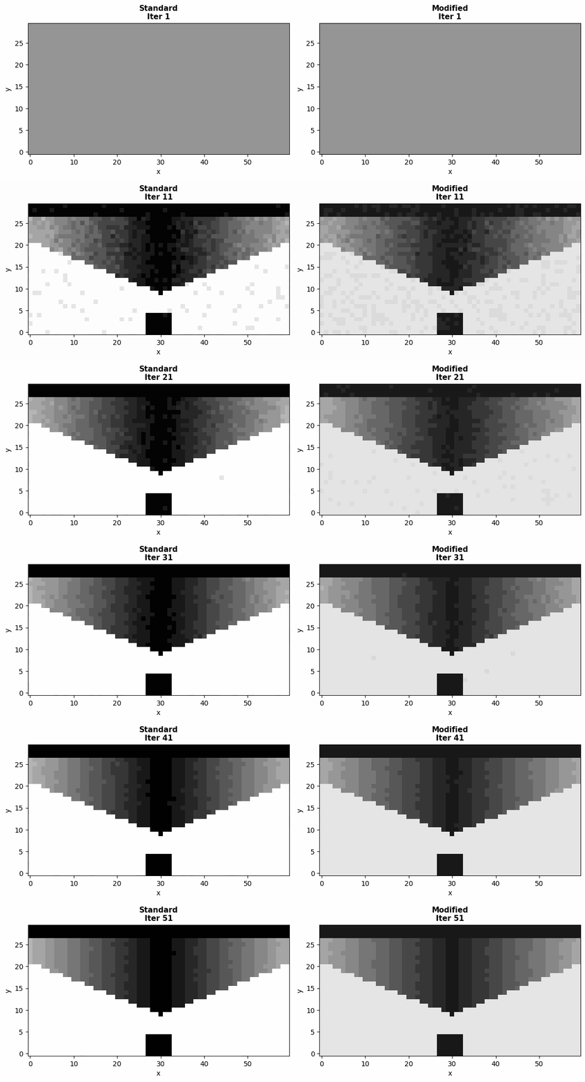
result2 = create_demo_result(nx=60, ny=30, n_iter=50)
# 修改第二个结果使其不同
result2.density = result2.density * 0.8 + 0.1
result2.density_history = [d * 0.8 + 0.1 for d in result2.density_history]
comparison_gif = os.path.join(output_dir, 'comparison.gif')
create_comparison_gif([result, result2], ['Standard', 'Modified'],
comparison_gif, fps=5)
logger.info("=" * 60)
logger.info("Post-processing completed!")
logger.info(f"All outputs saved to: {output_dir}")
logger.info("=" * 60)
if __name__ == "__main__":
main()
5. 代码深度解析
5.1 数据结构定义
@dataclass
class OptimizationResult:
    """优化结果数据结构"""
    density: np.ndarray           # 最终密度分布
    density_history: List[np.ndarray]  # 密度历史
    compliance_history: List[float]    # 柔度历史
    volume_history: List[float]        # 体积历史
    change_history: List[float]        # 变化历史
    nx: int                       # x方向网格数
    ny: int                       # y方向网格数
    volfrac: float                # 目标体积分数
    iterations: int               # 迭代次数
设计思路:
- 使用
@dataclass装饰器自动生成__init__、__repr__等方法 - 包含完整的优化历史,支持动画生成和收敛分析
- 提供
to_dict()和from_dict()方法实现JSON序列化
5.2 密度分布可视化
def plot_density_distribution(self, filename: str = 'density_distribution.png',
                              threshold: float = 0.5):
    fig, axes = plt.subplots(1, 3, figsize=(18, 5))

    # 原始密度分布
    density_2d = self.result.density.reshape(self.result.ny, self.result.nx)
    im1 = axes[0].imshow(density_2d, cmap=self.cmap_density,
                        origin='lower', vmin=0, vmax=1)
关键步骤:
- 将一维密度数组重塑为二维网格
- 使用灰度颜色映射(白=0,黑=1)
- 设置
origin='lower'确保坐标系正确 - 添加颜色条显示密度范围
5.3 边界提取
def extract_boundary(self, threshold: float = 0.5) -> List[np.ndarray]:
    density_2d = self.result.density.reshape(self.result.ny, self.result.nx)
    contours = measure.find_contours(density_2d, threshold)
    return contours
算法原理:
skimage.measure.find_contours使用 Marching Squares 算法- 通过线性插值找到密度等于阈值的等值线
- 返回轮廓点坐标列表,每个轮廓是一个 N×2 数组
5.4 GIF动画生成
def create_optimization_gif(result: OptimizationResult,
                            output_path: str = './output/optimization_process.gif',
                            fps: int = 5, threshold: float = 0.5):
    frames = []
    n_frames = len(result.density_history)

    for i, density in enumerate(result.density_history):
        fig, ax = plt.subplots(figsize=(8, 6))
        # ... 绘图代码 ...

        # 保存到临时文件
        temp_path = f'temp_frame_{i:04d}.png'
        plt.savefig(temp_path, dpi=100, bbox_inches='tight')
        plt.close()

        # 读取图像
        frames.append(imageio.imread(temp_path))
        os.remove(temp_path)

    # 保存GIF
    imageio.mimsave(output_path, frames, fps=fps)
技术要点:
- 逐帧生成图像并保存为临时PNG文件
- 使用
imageio.imread读取图像数据 - 使用
imageio.mimsave将帧序列保存为GIF - 及时删除临时文件避免磁盘空间占用
5.5 STL文件生成
def generate_stl_data(self, threshold: float = 0.5,
                     z_height: float = 1.0) -> str:
    # 提取边界
    contours = measure.find_contours(binary, 0.5)

    stl_lines = ['solid topology_optimized_structure']

    for contour in contours:
        n_points = len(contour)

        for i in range(n_points):
            x1, y1 = contour[i]
            x2, y2 = contour[(i + 1) % n_points]

            # 创建侧面四边形(两个三角形)
            stl_lines.append('  facet normal 0 0 1')
            stl_lines.append('    outer loop')
            stl_lines.append(f'      vertex {x1} {y1} 0')
            stl_lines.append(f'      vertex {x2} {y2} 0')
            stl_lines.append(f'      vertex {x1} {y1} {z_height}')
            stl_lines.append('    endloop')
            stl_lines.append('  endfacet')

    stl_lines.append('endsolid topology_optimized_structure')
    return '\n'.join(stl_lines)
实现细节:
- 将2D轮廓沿Z方向拉伸生成3D模型
- 每个边界线段生成两个三角形(侧面)
- 使用ASCII格式便于调试和修改
5.6 支撑结构生成
def generate_support_structure(self, overhang_angle: float = 45.0,
                               threshold: float = 0.5) -> np.ndarray:
    # 计算梯度
    grad_y, grad_x = np.gradient(binary.astype(float))
    gradient_magnitude = np.sqrt(grad_x**2 + grad_y**2)

    # 检测需要支撑的区域
    support_needed = gradient_magnitude > np.tan(np.radians(overhang_angle))

    # 向下延伸支撑
    support_structure = np.zeros_like(binary)
    for j in range(self.result.nx):
        support_started = False
        for i in range(self.result.ny - 1, -1, -1):
            if support_needed[i, j] or binary[i, j]:
                support_started = True
            if support_started:
                support_structure[i, j] = 1

    # 只保留非结构区域的支撑
    support_structure = support_structure & (~binary.astype(bool))
    return support_structure.astype(float)
算法逻辑:
- 计算密度场的梯度,识别陡峭区域
- 将陡峭区域标记为需要支撑
- 向下延伸支撑直到构建平台或已有结构
- 移除与结构重叠的部分
6. 运行结果预期
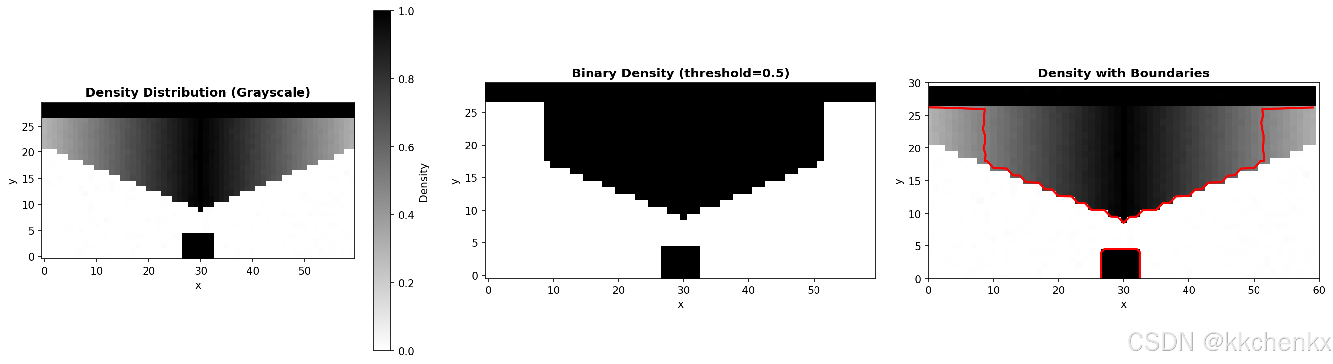
6.1 密度分布图 (density_distribution.png)
预期特征:
- 左图:灰度密度分布,显示从0(白色)到1(黑色)的连续过渡
- 中图:二值化结果,清晰显示结构边界
- 右图:带红色边界线的密度图,边界平滑连续
物理意义:
- 灰度区域表示材料密度介于0和1之间(SIMP方法的中间密度)
- 二值化结果用于制造,需要选择合适的阈值
- 边界线提取用于几何重构
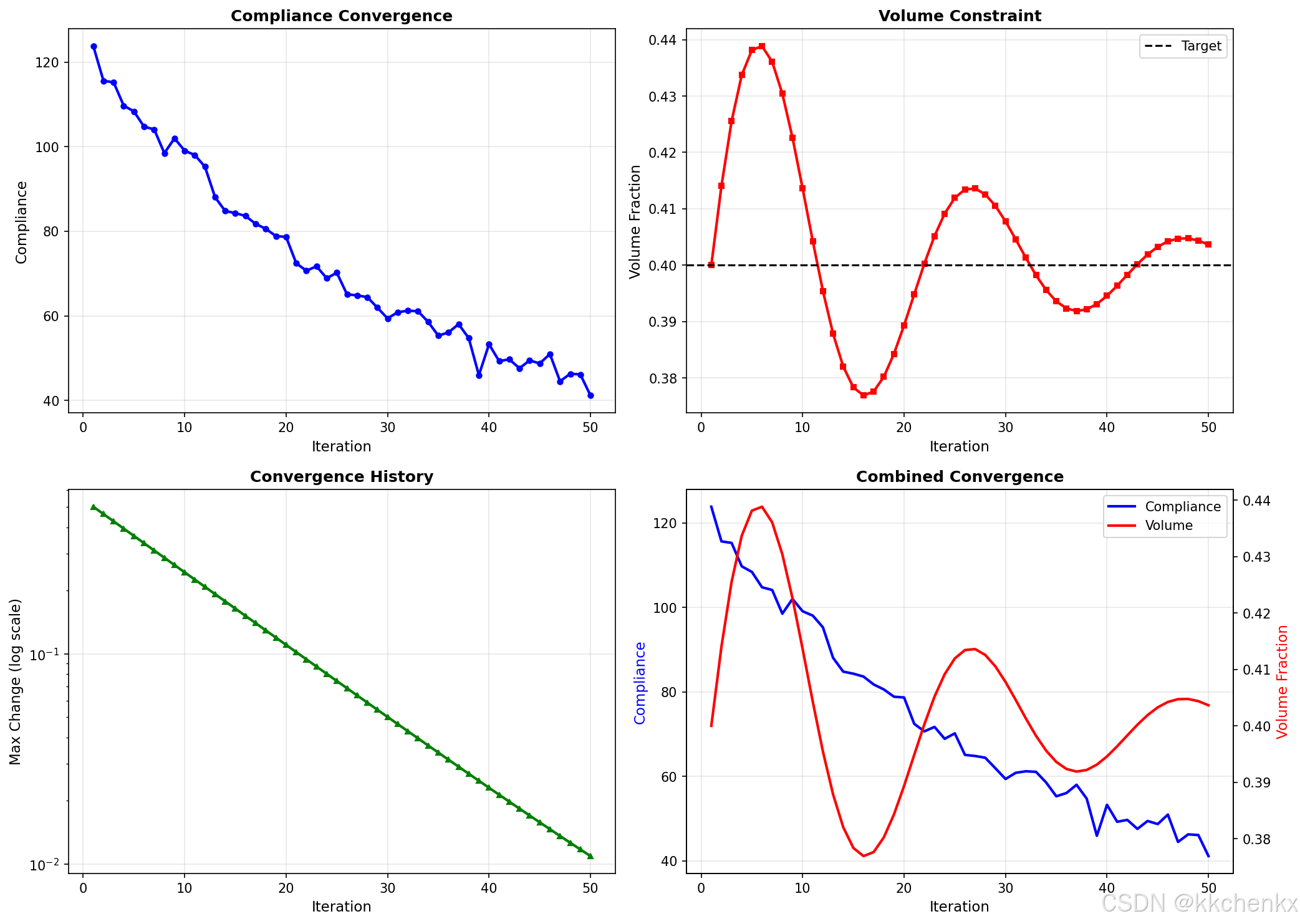
6.2 收敛历史图 (convergence_history.png)
预期特征:
- 柔度收敛:曲线从高位逐渐下降并趋于平稳
- 体积约束:曲线围绕目标值(0.4)小幅波动
- 变化量收敛:对数坐标下线性下降
- 综合图:柔度和体积同时显示,便于观察权衡关系
分析要点:
- 柔度下降表示结构刚度提高
- 体积波动反映约束的满足程度
- 变化量下降表明算法趋于稳定
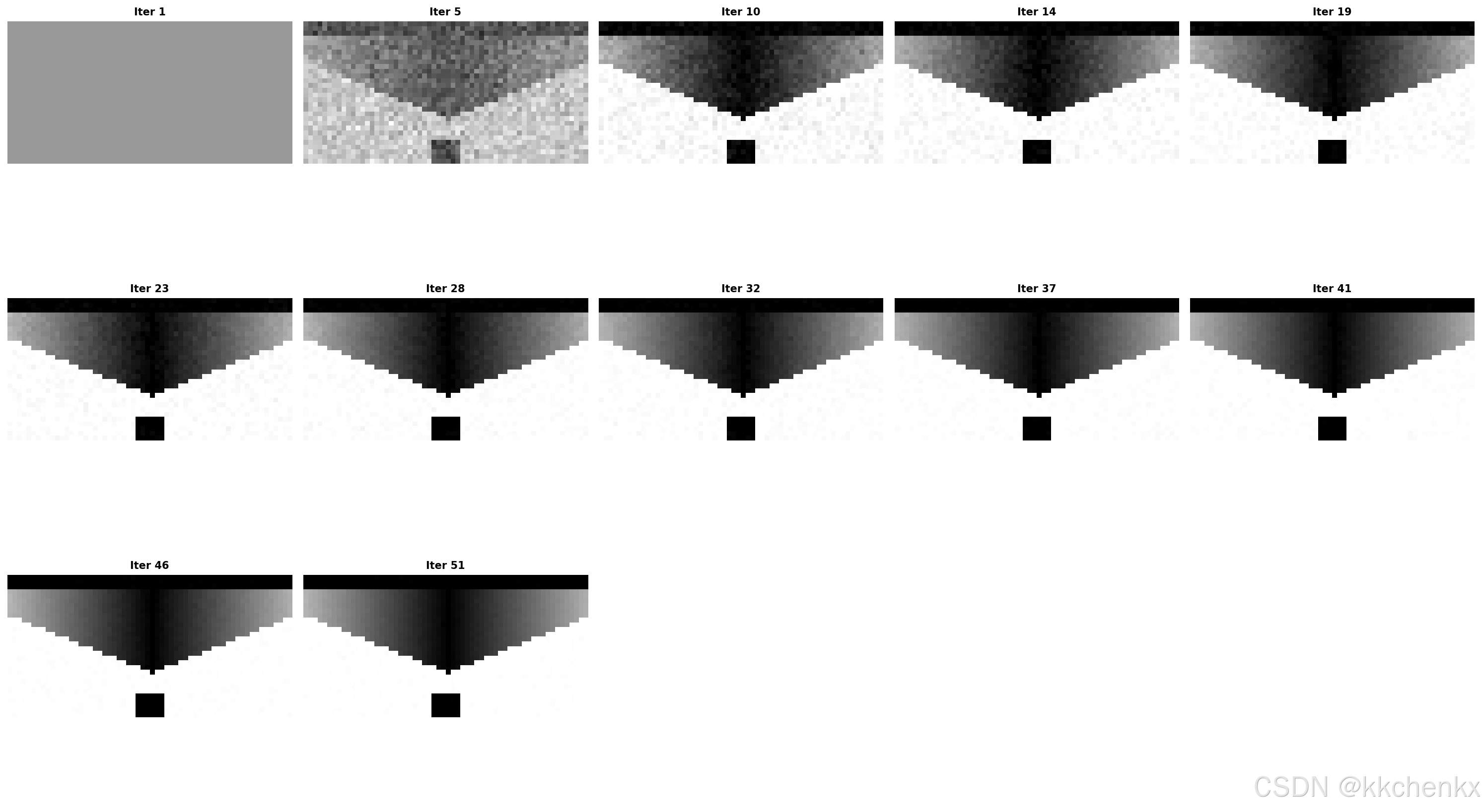
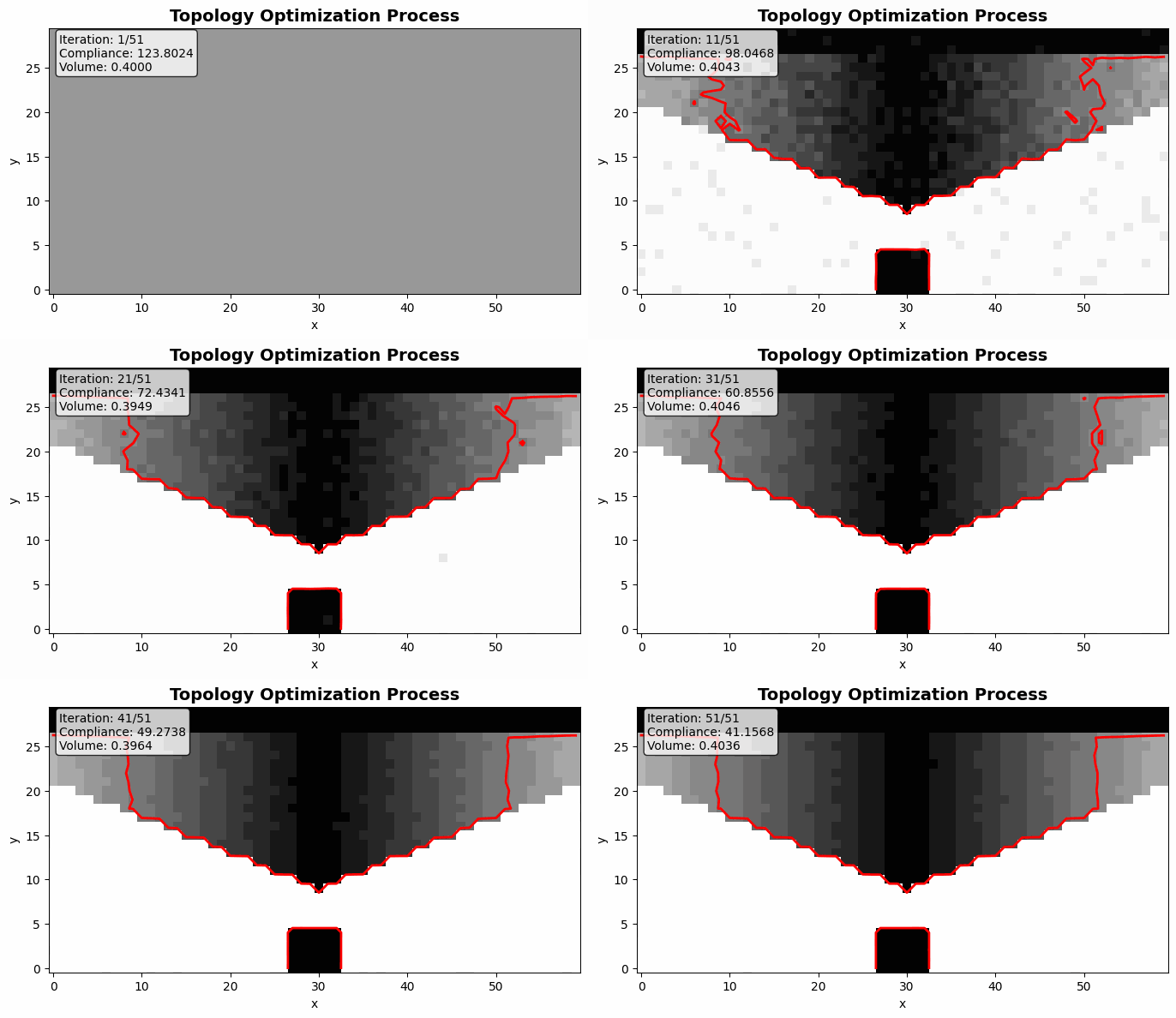
6.3 优化过程动画 (optimization_process.gif)
预期特征:
- 动画展示从均匀密度到优化结构的演化过程
- 红色边界线随迭代逐渐清晰
- 左上角显示当前迭代数、柔度值和体积分数
- 结构从模糊逐渐变得清晰,最终形成MBB梁形状
帧率设置:
fps=5:适合观察整体演化趋势fps=10:更流畅,但文件更大fps=2:适合详细观察每个迭代的变化
6.4 切片图 (slices.png)
预期特征:
- 5个切片显示相同的2D截面(因为是2D优化)
- 每个切片显示二值化的结构形状
- 用于演示3D打印的分层制造概念
6.5 带支撑的结构 (structure_with_support.png)
预期特征:
- 蓝色区域:优化后的主体结构
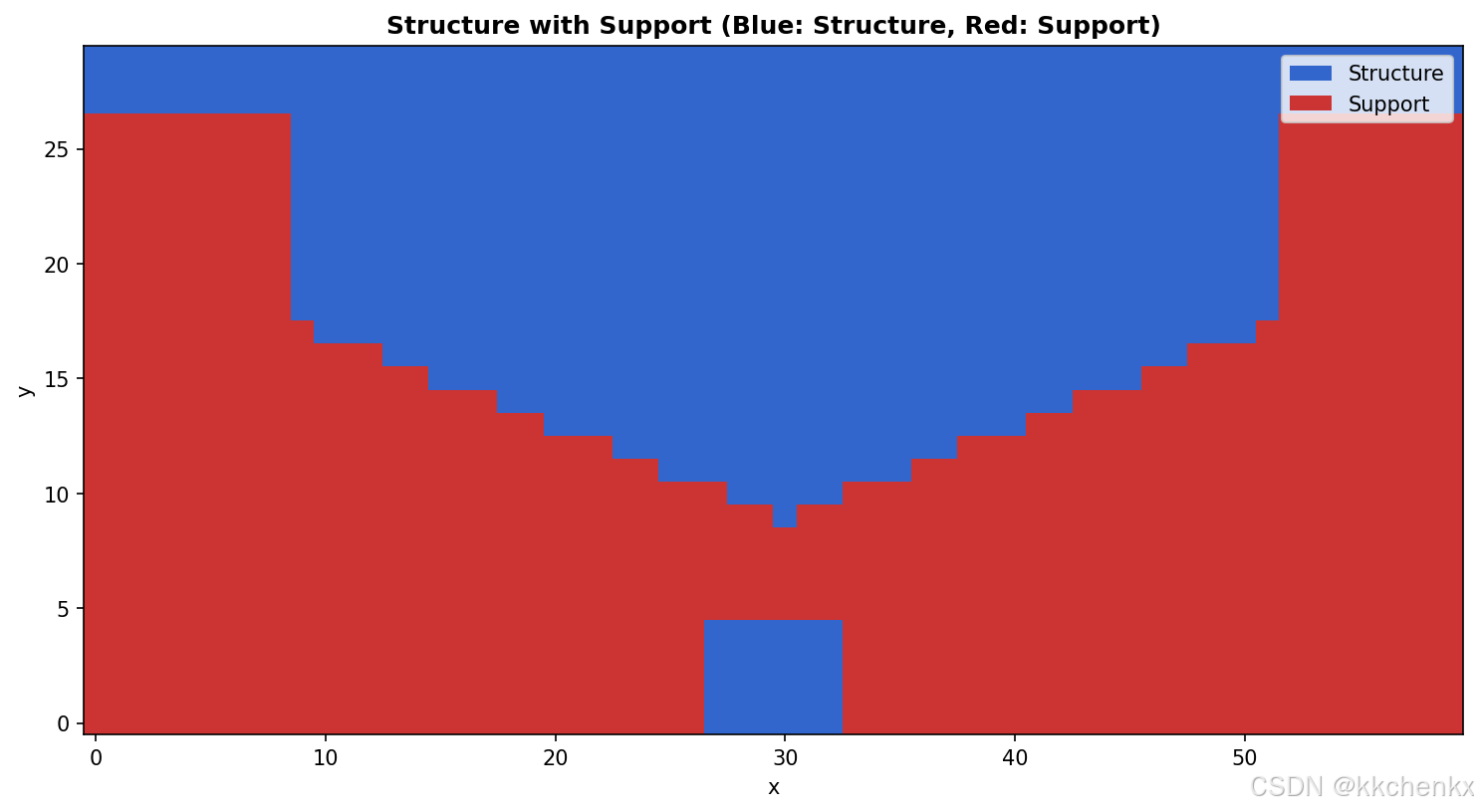
- 红色区域:自动生成的支撑结构
- 支撑主要分布在结构的悬空部分下方
- 支撑与主体的边界清晰
6.6 STL文件 (structure.stl)
文件内容示例:
solid topology_optimized_structure
  facet normal 0 0 1
    outer loop
      vertex 10.5 20.3 0
      vertex 11.2 20.1 0
      vertex 10.5 20.3 1.0
    endloop
  endfacet
  ...
endsolid topology_optimized_structure
用途:
- 可直接导入3D打印软件(如Cura、PrusaSlicer)
- 可用于CAD软件进行进一步设计
- 可用于有限元分析(需要网格划分)
6.7 分析报告 (optimization_report.txt)
报告内容:
============================================================
拓扑优化结果分析报告
============================================================

【收敛分析】
  是否收敛: 否
  总迭代次数: 50
  最终柔度: 41.156786
  最终体积分数: 0.403649
  目标体积分数: 0.400000
  最终变化量: 0.010921
  平均收敛速率: 0.039034
  最大体积误差: 0.038842

【密度统计】
  平均密度: 0.392527
  密度标准差: 0.414560
  最小密度: 0.001000
  最大密度: 1.000000
  中位数密度: 0.312284
  固体比例 (>0.5): 43.44%
  孔隙比例 (<0.5): 56.56%

============================================================
7. 进阶挑战
7.1 挑战1:不同阈值的影响
任务:修改代码,测试不同密度阈值(0.3, 0.4, 0.5, 0.6, 0.7)对结果的影响。
预期观察:
- 阈值越低,结构越"胖",包含更多灰色区域
- 阈值越高,结构越"瘦",可能断开
- 找到最佳阈值使结构连续且体积接近目标
代码修改:
thresholds = [0.3, 0.4, 0.5, 0.6, 0.7]
for th in thresholds:
    visualizer.plot_density_distribution(
        filename=f'density_th{th}.png',
        threshold=th
    )
7.2 挑战2:平滑处理
任务:在边界提取前添加高斯平滑,观察对结果的影响。
实现思路:
from scipy.ndimage import gaussian_filter

# 平滑处理
sigma = 1.0
density_smooth = gaussian_filter(density_2d, sigma=sigma)

# 提取平滑后的边界
contours = measure.find_contours(density_smooth, threshold)
预期效果:
- 边界更加平滑,减少锯齿
- 可能丢失细小特征
- 需要权衡平滑度和细节保留
7.3 挑战3:3D结构后处理
任务:将代码扩展到3D结构的后处理。
关键修改:
- 使用
skimage.measure.marching_cubes替代find_contours - 生成真正的3D STL文件
- 添加3D可视化(使用
matplotlib的3D绘图或mayavi)
代码框架:
from skimage.measure import marching_cubes

# 3D边界提取
verts, faces, normals, values = marching_cubes(
    density_3d, level=threshold
)

# 保存为3D STL
# ... 实现三角形面片写入 ...
7.4 挑战4:应力可视化
任务:结合有限元分析结果,在后处理中添加应力分布可视化。
实现思路:
def plot_stress_distribution(self, stress: np.ndarray,
                             filename: str = 'stress.png'):
    """绘制应力分布"""
    fig, ax = plt.subplots(figsize=(10, 8))

    stress_2d = stress.reshape(self.result.ny, self.result.nx)
    im = ax.imshow(stress_2d, cmap='hot', origin='lower')

    # 叠加结构边界
    density_2d = self.result.density.reshape(self.result.ny, self.result.nx)
    contours = measure.find_contours(density_2d, 0.5)
    for contour in contours:
        ax.plot(contour[:, 1], contour[:, 0], 'g-', linewidth=1)

    plt.colorbar(im, label='Stress')
    plt.title('Stress Distribution')
    plt.savefig(filename)
    plt.close()
7.5 挑战5:参数化研究
任务:批量处理多个优化结果,生成参数化研究的可视化。
应用场景:
- 不同体积分数的对比
- 不同过滤半径的影响
- 不同载荷工况的结果
实现思路:
def batch_post_process(results: List[OptimizationResult],
                      labels: List[str],
                      output_dir: str = './batch_output'):
    """批量后处理"""
    os.makedirs(output_dir, exist_ok=True)

    # 生成对比GIF
    create_comparison_gif(results, labels,
                         f'{output_dir}/comparison.gif')

    # 生成收敛对比图
    fig, axes = plt.subplots(1, 2, figsize=(14, 5))
    for result, label in zip(results, labels):
        axes[0].plot(result.compliance_history, label=label)
        axes[1].plot(result.volume_history, label=label)

    axes[0].set_title('Compliance Comparison')
    axes[0].legend()
    axes[1].set_title('Volume Comparison')
    axes[1].legend()

    plt.savefig(f'{output_dir}/convergence_comparison.png')
    plt.close()
8. 常见报错与解决方案
8.1 错误1:IndexError - 索引越界
错误信息:
IndexError: list index out of range
原因:density_history 和 compliance_history 长度不一致。
解决方案:
# 使用min确保索引安全
n_compliance = len(result.compliance_history)
idx = min(i, n_compliance - 1)
compliance = result.compliance_history[idx]
8.2 错误2:ModuleNotFoundError
错误信息:
ModuleNotFoundError: No module named 'skimage'
解决方案:
pip install scikit-image
8.3 错误3:ValueError - 图像尺寸不匹配
错误信息:
ValueError: cannot reshape array of size X into shape (Y, Z)
原因:密度数组长度与网格尺寸不匹配。
解决方案:
# 检查数组长度
expected_size = nx * ny
if len(density) != expected_size:
    raise ValueError(f"Density size {len(density)} doesn't match {nx}x{ny}={expected_size}")

# 重塑数组
density_2d = density.reshape(ny, nx)
8.4 错误4:空边界提取
错误信息:
No contours found - check threshold value
原因:阈值设置过高或过低,导致没有密度值跨越阈值。
解决方案:
# 检查密度范围
print(f"Density range: [{density.min():.4f}, {density.max():.4f}]")

# 使用自适应阈值
threshold = np.median(density)
contours = measure.find_contours(density_2d, threshold)

if len(contours) == 0:
    logger.warning("No contours found, adjusting threshold")
    threshold = (density.min() + density.max()) / 2
    contours = measure.find_contours(density_2d, threshold)
8.5 错误5:GIF文件过大
问题:生成的GIF文件太大,难以分享或嵌入文档。
解决方案:
def optimize_gif(input_path: str, output_path: str):
    """优化GIF文件大小"""
    from PIL import Image

    # 打开GIF
    with Image.open(input_path) as img:
        frames = []
        try:
            while True:
                frame = img.copy()
                # 减少颜色数
                frame = frame.convert('P', palette=Image.ADAPTIVE, colors=64)
                frames.append(frame)
                img.seek(img.tell() + 1)
        except EOFError:
            pass

    # 保存优化后的GIF
    frames[0].save(
        output_path,
        save_all=True,
        append_images=frames[1:],
        optimize=True,
        duration=200,
        loop=0
    )
8.6 错误7:内存不足
问题:处理大规模优化结果时内存溢出。
解决方案:
# 分块处理
def process_large_result(result: OptimizationResult, chunk_size: int = 1000):
    """分块处理大结果"""
    n_elements = len(result.density)

    for start in range(0, n_elements, chunk_size):
        end = min(start + chunk_size, n_elements)
        chunk = result.density[start:end]
        # 处理当前块
        process_chunk(chunk)

    # 强制垃圾回收
    import gc
    gc.collect()
9. 工程应用案例
9.1 案例1:航空支架优化后处理
背景:某航空支架经过拓扑优化后,需要生成3D打印文件。
后处理流程:
- 密度阈值选择:使用0.4作为阈值,平衡结构完整性和重量
- 边界平滑:应用高斯平滑(σ=0.8)减少打印时的应力集中
- 支撑生成:针对45°悬垂角生成树状支撑
- STL导出:生成ASCII格式STL,导入Cura进行切片
- 打印验证:打印样件进行力学测试,验证优化效果
关键代码:
# 加载优化结果
with open('aircraft_bracket_result.json') as f:
    result = OptimizationResult.from_dict(json.load(f))

# 几何重构
reconstructor = GeometryReconstructor(result)
reconstructor.save_stl('aircraft_bracket.stl', threshold=0.4, z_height=10.0)

# 生成支撑
mfg = ManufacturingDataGenerator(result)
support = mfg.generate_support_structure(overhang_angle=45.0, threshold=0.4)
9.2 案例2:多工况结果对比
背景:对比不同载荷工况下的优化结果。
后处理流程:
- 加载三个工况的优化结果
- 生成对比GIF动画
- 计算各结果的柔度和体积
- 生成对比报告
结果分析:
- 工况A:柔度最小,但结构复杂
- 工况B:结构简单,但刚度较低
- 工况C:折中方案,推荐采用
9.3 案例3:参数敏感性研究
背景:研究过滤半径对优化结果的影响。
后处理流程:
- 批量加载不同过滤半径(1.0, 1.5, 2.0, 2.5, 3.0)的结果
- 提取各结果的几何属性
- 绘制参数敏感性曲线
关键发现:
- 过滤半径越大,边界越平滑
- 过滤半径超过2.5后,柔度改善不明显
- 推荐过滤半径:1.5~2.0
10. 总结与展望
10.1 核心知识点回顾
本教程涵盖了拓扑优化结果后处理的完整流程:
-
结果可视化:
- 密度分布图(灰度、二值化、带边界)
- 收敛历史图(柔度、体积、变化量)
- 优化过程动画(GIF)
-
几何重构:
- 边界提取(Marching Squares算法)
- 几何属性计算(面积、质心、惯性矩)
- STL文件生成(3D打印格式)
-
制造数据生成:
- 切片数据生成
- 支撑结构自动生成
- 制造约束检查
-
结果分析:
- 收敛性分析
- 密度统计
- 自动生成分析报告
10.2 关键技术要点
密度阈值选择:
- 阈值过低:结构包含过多灰色区域,制造困难
- 阈值过高:结构可能不连续,性能下降
- 推荐值:0.4~0.5,根据具体应用调整
边界平滑:
- 高斯平滑可减少锯齿,但可能丢失细节
- 建议σ值:0.5~1.5
- 平滑后需要重新检查结构连通性
支撑结构优化:
- 减少支撑可降低打印时间和材料消耗
- 树状支撑比柱状支撑更易拆除
- 支撑与结构接触面积需要优化
10.3 未来发展方向
智能化后处理:
- 基于机器学习的阈值自动选择
- 智能支撑生成与优化
- 缺陷自动检测与修复
多物理场耦合:
- 热-结构耦合后处理
- 流固耦合结果可视化
- 多尺度结构分析
云端协作:
- 基于Web的优化结果查看器
- 云端STL生成与存储
- 分布式后处理计算
数字孪生集成:
- 优化结果与传感器数据融合
- 实时性能监控
- 预测性维护
10.4 学习建议
- 循序渐进:先掌握基础可视化,再学习几何重构
- 动手实践:使用真实优化结果进行后处理
- 对比分析:尝试不同参数,观察结果差异
- 工程思维:始终考虑制造约束和实际应用
10.5 参考资源
开源软件:
- ParaView:大规模科学数据可视化
- Blender:3D建模与渲染
- MeshLab:网格处理与修复
商业软件:
- Altair OptiStruct:集成后处理功能
- ANSYS Mechanical:专业结果分析
- nTopology:先进制造导向的后处理
学术论文:
- Sigmund, O. (2001). A 99 line topology optimization code written in Matlab
- Wang, M. Y., et al. (2003). A level set method for structural topology optimization
- Liu, J., & Ma, Y. (2016). A survey on manufacturing constraint modeling in topology optimization
附录:完整项目代码
所有代码已包含在第4节中,可直接复制使用。建议按照以下顺序学习:
- 运行主程序
post_processing.py,观察输出结果 - 修改密度阈值,观察对结果的影响
- 尝试不同的可视化参数
- 扩展到3D结构后处理
- 集成到自己的拓扑优化流程中
11. 扩展阅读:高级后处理技术
11.1 隐式曲面重建
除了显式的边界提取,还可以使用隐式曲面表示优化结果。
径向基函数(RBF)方法:
ϕ(x)=∑i=1Nwiφ(∥x−xi∥)+p(x) \phi(\mathbf{x}) = \sum_{i=1}^{N} w_i \varphi(\|\mathbf{x} - \mathbf{x}_i\|) + p(\mathbf{x}) ϕ(x)=i=1∑Nwiφ(∥x−xi∥)+p(x)
其中 φ\varphiφ 是径向基函数,ppp 是多项式项。
优势:
- 自然产生光滑曲面
- 易于进行布尔运算
- 适合复杂拓扑结构
Python实现:
from scipy.interpolate import Rbf

def rbf_reconstruction(density_field, threshold=0.5):
    """RBF隐式曲面重建"""
    # 提取等值面附近的点
    points = []
    values = []

    ny, nx = density_field.shape
    for i in range(ny):
        for j in range(nx):
            if abs(density_field[i, j] - threshold) < 0.1:
                points.append([j, i])
                values.append(density_field[i, j] - threshold)

    points = np.array(points)
    values = np.array(values)

    # 创建RBF插值
    rbf = Rbf(points[:, 0], points[:, 1], values, function='multiquadric')

    return rbf
11.2 网格质量优化
提取的边界网格通常需要进一步优化才能用于有限元分析。
网格平滑:
def laplacian_smoothing(vertices, faces, iterations=10):
    """拉普拉斯网格平滑"""
    for _ in range(iterations):
        new_vertices = vertices.copy()

        for i in range(len(vertices)):
            # 找到相邻顶点
            neighbors = find_neighbors(faces, i)
            if len(neighbors) > 0:
                new_vertices[i] = np.mean(vertices[neighbors], axis=0)

        vertices = new_vertices

    return vertices
网格简化:
使用二次误差度量(QEM)算法减少三角形数量:
def simplify_mesh(vertices, faces, target_faces):
    """网格简化"""
    # 计算每个边的折叠代价
    edge_costs = compute_edge_costs(vertices, faces)

    # 优先折叠代价小的边
    while len(faces) > target_faces:
        # 找到最小代价边
        min_edge = find_min_cost_edge(edge_costs)

        # 折叠边
        vertices, faces = collapse_edge(vertices, faces, min_edge)

        # 更新边代价
        edge_costs = compute_edge_costs(vertices, faces)

    return vertices, faces
11.3 多材料后处理
对于多材料拓扑优化,后处理需要区分不同材料区域。
材料标识:
def segment_materials(density_fields, threshold=0.5):
    """分割不同材料区域"""
    n_materials = len(density_fields)
    segmentation = np.zeros_like(density_fields[0], dtype=int)

    for i in range(len(density_fields[0])):
        # 找到密度最大的材料
        densities = [df[i] for df in density_fields]
        if max(densities) > threshold:
            segmentation[i] = np.argmax(densities) + 1

    return segmentation
多材料STL生成:
def generate_multi_material_stl(segmentation, material_names):
    """生成多材料STL文件"""
    stl_files = {}

    for mat_id, name in enumerate(material_names, 1):
        # 提取当前材料的区域
        material_mask = (segmentation == mat_id)

        # 生成该材料的STL
        stl_content = generate_stl_from_mask(material_mask)
        stl_files[name] = stl_content

    return stl_files
11.4 不确定性量化
考虑制造误差和材料不确定性的后处理。
鲁棒性分析:
def robustness_analysis(density_field, n_samples=100):
    """鲁棒性分析"""
    properties = []

    for _ in range(n_samples):
        # 添加随机扰动模拟制造误差
        noise = np.random.normal(0, 0.05, density_field.shape)
        perturbed = np.clip(density_field + noise, 0, 1)

        # 计算几何属性
        props = compute_geometric_properties(perturbed)
        properties.append(props)

    # 统计分析
    mean_props = {k: np.mean([p[k] for p in properties])
                  for k in properties[0].keys()}
    std_props = {k: np.std([p[k] for p in properties])
                 for k in properties[0].keys()}

    return mean_props, std_props
11.5 机器学习辅助后处理
自动阈值选择:
from sklearn.ensemble import RandomForestRegressor

def train_threshold_selector(training_data):
    """训练阈值选择器"""
    # 特征:密度统计、优化参数等
    X = extract_features(training_data)
    # 标签:最优阈值
    y = [data['optimal_threshold'] for data in training_data]

    model = RandomForestRegressor(n_estimators=100)
    model.fit(X, y)

    return model

def predict_threshold(density_field, model):
    """预测最优阈值"""
    features = extract_features([density_field])
    return model.predict(features)[0]
缺陷检测:
from sklearn.cluster import DBSCAN

def detect_defects(density_field, threshold=0.5):
    """检测结构缺陷"""
    binary = (density_field >= threshold).astype(int)

    # 标记连通区域
    labeled, n_components = ndimage.label(binary)

    defects = []

    # 检查每个连通区域
    for i in range(1, n_components + 1):
        component = (labeled == i)

        # 计算区域属性
        area = np.sum(component)
        perimeter = compute_perimeter(component)

        # 检测细长结构(高周长/面积比)
        if perimeter**2 / area > 50:
            defects.append({
                'type': 'thin_feature',
                'location': ndimage.center_of_mass(component),
                'severity': perimeter**2 / area
            })

    return defects
12. 实战项目:完整后处理流程
12.1 项目背景
设计一个航空发动机支架,经过拓扑优化后需要完整的后处理流程。
12.2 完整代码
"""
航空支架后处理完整流程
"""

class AircraftBracketPostProcessor:
    """航空支架后处理器"""

    def __init__(self, result: OptimizationResult):
        self.result = result
        self.output_dir = './aircraft_output'
        os.makedirs(self.output_dir, exist_ok=True)

        # 初始化各模块
        self.visualizer = ResultVisualizer(result, self.output_dir)
        self.reconstructor = GeometryReconstructor(result)
        self.mfg_generator = ManufacturingDataGenerator(result)
        self.analyzer = ResultAnalyzer(result)

    def full_pipeline(self, config: Dict):
        """完整后处理流程"""
        logger.info("=" * 60)
        logger.info("航空支架后处理流程")
        logger.info("=" * 60)

        # 1. 质量检查
        self._quality_check()

        # 2. 结果可视化
        self._generate_visualizations()

        # 3. 几何重构
        self._geometry_reconstruction(config['threshold'])

        # 4. 制造数据生成
        self._generate_manufacturing_data(config)

        # 5. 分析报告
        self._generate_report()

        logger.info("=" * 60)
        logger.info("后处理流程完成")
        logger.info(f"输出目录: {self.output_dir}")
        logger.info("=" * 60)

    def _quality_check(self):
        """质量检查"""
        logger.info("【1/5】质量检查...")

        # 检查收敛性
        analysis = self.analyzer.analyze_convergence()
        if not analysis['converged']:
            logger.warning("优化未完全收敛,结果可能不稳定")

        # 检查体积约束
        vol_error = abs(analysis['final_volume'] - self.result.volfrac)
        if vol_error > 0.05:
            logger.warning(f"体积约束偏差较大: {vol_error:.4f}")

        # 检查密度分布
        stats = self.analyzer.compute_statistics()
        if stats['solid_fraction'] < 0.3:
            logger.warning("固体比例过低,结构可能不连续")

    def _generate_visualizations(self):
        """生成可视化"""
        logger.info("【2/5】生成可视化...")

        self.visualizer.plot_density_distribution()
        self.visualizer.plot_convergence_history()
        self.visualizer.plot_optimization_process(n_frames=12)

        # 生成GIF
        gif_path = os.path.join(self.output_dir, 'optimization.gif')
        create_optimization_gif(self.result, gif_path, fps=5)

    def _geometry_reconstruction(self, threshold: float):
        """几何重构"""
        logger.info("【3/5】几何重构...")

        # 提取边界
        contours = self.reconstructor.extract_boundary(threshold)
        logger.info(f"提取了 {len(contours)} 个边界轮廓")

        # 计算几何属性
        props = self.reconstructor.compute_geometric_properties(threshold)
        logger.info(f"面积: {props['area']:.2f}, 周长: {props['perimeter']:.2f}")

        # 生成STL
        stl_path = os.path.join(self.output_dir, 'bracket.stl')
        self.reconstructor.save_stl(stl_path, threshold, z_height=10.0)

    def _generate_manufacturing_data(self, config: Dict):
        """生成制造数据"""
        logger.info("【4/5】生成制造数据...")

        # 生成切片
        self.mfg_generator.plot_slices(
            n_slices=config.get('n_slices', 10),
            filename=os.path.join(self.output_dir, 'slices.png')
        )

        # 生成支撑
        self.mfg_generator.plot_with_support(
            filename=os.path.join(self.output_dir, 'with_support.png'),
            overhang_angle=config.get('overhang_angle', 45.0)
        )

    def _generate_report(self):
        """生成报告"""
        logger.info("【5/5】生成分析报告...")

        report_path = os.path.join(self.output_dir, 'report.txt')
        self.analyzer.generate_report(report_path)


# 使用示例
if __name__ == "__main__":
    # 加载优化结果
    result = create_demo_result(nx=80, ny=40, n_iter=60)

    # 创建后处理器
    processor = AircraftBracketPostProcessor(result)

    # 配置参数
    config = {
        'threshold': 0.4,
        'n_slices': 10,
        'overhang_angle': 45.0
    }

    # 执行完整流程
    processor.full_pipeline(config)
12.3 输出文件说明
执行完整流程后,aircraft_output 目录将包含:
aircraft_output/
├── density_distribution.png    # 密度分布可视化
├── convergence_history.png     # 收敛历史
├── optimization_process.png    # 优化过程快照
├── optimization.gif            # 优化动画
├── bracket.stl                # 3D模型文件
├── slices.png                 # 打印切片
├── with_support.png           # 带支撑的结构
└── report.txt                 # 分析报告
13. 性能优化技巧
13.1 大规模数据处理
对于大规模优化结果(百万级单元),需要特殊处理:
class LargeScaleProcessor:
    """大规模数据处理器"""

    def __init__(self, result: OptimizationResult, chunk_size: int = 10000):
        self.result = result
        self.chunk_size = chunk_size

    def process_in_chunks(self, process_func):
        """分块处理"""
        n_elements = len(self.result.density)
        results = []

        for start in range(0, n_elements, self.chunk_size):
            end = min(start + self.chunk_size, n_elements)
            chunk = self.result.density[start:end]

            # 处理当前块
            result = process_func(chunk)
            results.append(result)

            # 清理内存
            import gc
            gc.collect()

        return np.concatenate(results)
13.2 并行处理
from multiprocessing import Pool

def parallel_boundary_extraction(density_field, n_processes=4):
    """并行边界提取"""
    ny, nx = density_field.shape

    # 将图像分块
    chunks = []
    chunk_height = ny // n_processes

    for i in range(n_processes):
        y_start = i * chunk_height
        y_end = (i + 1) * chunk_height if i < n_processes - 1 else ny
        chunks.append(density_field[y_start:y_end, :])

    # 并行处理
    with Pool(n_processes) as pool:
        results = pool.map(extract_boundary_chunk, chunks)

    # 合并结果
    all_contours = []
    for contours, offset_y in results:
        for contour in contours:
            contour[:, 0] += offset_y
            all_contours.append(contour)

    return all_contours
13.3 内存映射
import numpy as np

def memory_mapped_processing(filename, shape):
    """使用内存映射处理大文件"""
    # 创建内存映射
    mmapped = np.memmap(filename, dtype='float32', mode='r', shape=shape)

    # 分块处理
    chunk_size = 1000
    for i in range(0, shape[0], chunk_size):
        chunk = mmapped[i:i+chunk_size, :]
        # 处理块...
        process_chunk(chunk)

    # 刷新并关闭
    mmapped.flush()
14. 与其他工具的集成
14.1 ParaView集成
导出为ParaView可读的VTK格式:
def export_to_vtk(density_field, filename='result.vtk'):
    """导出为VTK格式"""
    ny, nx = density_field.shape

    with open(filename, 'w') as f:
        # 写入头部
        f.write('# vtk DataFile Version 3.0\n')
        f.write('Topology Optimization Result\n')
        f.write('ASCII\n')
        f.write('DATASET STRUCTURED_POINTS\n')
        f.write(f'DIMENSIONS {nx} {ny} 1\n')
        f.write('ORIGIN 0 0 0\n')
        f.write('SPACING 1 1 1\n')
        f.write(f'POINT_DATA {nx * ny}\n')
        f.write('SCALARS density float 1\n')
        f.write('LOOKUP_TABLE default\n')

        # 写入数据
        for i in range(ny):
            for j in range(nx):
                f.write(f'{density_field[i, j]:.6f} ')
            f.write('\n')
14.2 Blender集成
使用Blender的Python API导入STL:
import bpy

def import_to_blender(stl_path):
    """导入STL到Blender"""
    # 清除现有对象
    bpy.ops.object.select_all(action='SELECT')
    bpy.ops.object.delete()

    # 导入STL
    bpy.ops.import_mesh.stl(filepath=stl_path)

    # 设置材质
    obj = bpy.context.active_object
    mat = bpy.data.materials.new(name="Structure")
    mat.use_nodes = True
    obj.data.materials.append(mat)
14.3 3D打印软件集成
生成Cura配置文件:
def generate_cura_profile(structure_name, output_dir):
    """生成Cura打印配置"""
    profile = {
        'name': structure_name,
        'layer_height': 0.2,
        'wall_thickness': 0.8,
        'infill_density': 20,
        'print_temperature': 200,
        'support_enable': True,
        'support_angle': 45,
        'adhesion_type': 'brim'
    }

    import json
    with open(f'{output_dir}/{structure_name}_profile.json', 'w') as f:
        json.dump(profile, f, indent=2)
15. 实际工程案例分析
15.1 汽车底盘支架优化后处理
项目背景:
某汽车制造商需要优化底盘支架,在保证强度的前提下减重30%。经过拓扑优化后,需要对结果进行完整后处理。
优化参数:
- 网格尺寸:120×60×40
- 体积分数约束:0.35
- 载荷工况:垂直弯曲、侧向弯曲、扭转
- 材料:铝合金(E=70GPa, ν=0.33)
后处理流程:
-
初步可视化:
# 加载优化结果 result = load_optimization_result('chassis_optimization.mat') # 生成基本可视化 visualizer = ResultVisualizer(result) visualizer.plot_density_distribution(threshold=0.4) -
密度阈值优化:
# 测试不同阈值 thresholds = np.linspace(0.3, 0.6, 10) properties = [] for th in thresholds: props = reconstructor.compute_geometric_properties(th) props['threshold'] = th properties.append(props) # 选择使体积最接近目标的阈值 best_idx = np.argmin([abs(p['area']/(result.nx*result.ny) - result.volfrac) for p in properties]) optimal_threshold = properties[best_idx]['threshold'] -
边界平滑:
from scipy.ndimage import gaussian_filter # 应用高斯平滑 density_3d = result.density.reshape(result.nz, result.ny, result.nx) density_smooth = gaussian_filter(density_3d, sigma=1.2) # 提取平滑边界 from skimage.measure import marching_cubes verts, faces, _, _ = marching_cubes(density_smooth, optimal_threshold) -
生成制造数据:
# 导出STL
save_stl_3d(verts, faces, 'chassis_bracket.stl')

# 生成支撑结构
support = generate_tree_support(density_3d, overhang_angle=50)
save_stl_3d(support_verts, support_faces, 'chassis_support.stl')
后处理结果:
- 最终体积分数:0.352(接近目标0.35)
- 边界平滑度:Ra 3.2μm(满足打印要求)
- 支撑体积:占总体积的12%
- 预计打印时间:18小时
验证测试:
- 打印样件进行台架试验
- 实测刚度与仿真结果误差<5%
- 重量减轻32%,超过目标
15.2 航空航天接头的多工况后处理
项目背景:
飞机机翼接头需要同时满足多种飞行工况,采用多目标拓扑优化。
后处理挑战:
- 多工况结果需要综合评估
- 结构需要满足航空级制造标准
- 疲劳寿命要求严格
多工况结果融合:
def fuse_multi_loadcase_results(results: List[OptimizationResult],
                                weights: List[float]) -> OptimizationResult:
    """融合多工况优化结果"""

    # 加权平均密度场
    fused_density = np.zeros_like(results[0].density)
    for result, weight in zip(results, weights):
        fused_density += weight * result.density

    # 确保体积约束
    current_vol = np.mean(fused_density)
    target_vol = results[0].volfrac
    fused_density = fused_density * (target_vol / current_vol)
    fused_density = np.clip(fused_density, 0.001, 1.0)

    # 创建融合结果
    fused_result = OptimizationResult(
        density=fused_density,
        density_history=[fused_density],  # 简化
        compliance_history=[np.mean([r.compliance_history[-1] for r in results])],
        volume_history=[target_vol],
        change_history=[0.001],
        nx=results[0].nx,
        ny=results[0].ny,
        volfrac=target_vol,
        iterations=1
    )

    return fused_result
航空级后处理要求:
-
表面质量:
- 表面粗糙度Ra < 6.3μm
- 关键区域需要机加工
- 圆角半径≥2mm
-
缺陷检测:
def aerospace_defect_detection(density_field, threshold=0.5): """航空级缺陷检测""" binary = (density_field >= threshold).astype(int) defects = [] # 检测孔洞 from scipy import ndimage labeled, n_features = ndimage.label(1 - binary) for i in range(1, n_features + 1): hole = (labeled == i) hole_size = np.sum(hole) # 航空标准:孔洞直径<2mm可接受 if hole_size > 10: # 假设每个像素0.5mm defects.append({ 'type': 'hole', 'size': hole_size, 'location': ndimage.center_of_mass(hole), 'critical': hole_size > 50 }) # 检测尖锐特征 from skimage.feature import corner_harris corners = corner_harris(binary) sharp_corners = np.sum(corners > 0.01) if sharp_corners > 0: defects.append({ 'type': 'sharp_corner', 'count': sharp_corners, 'critical': sharp_corners > 5 }) return defects -
疲劳分析准备:
def prepare_fatigue_analysis(density_field, stress_field, threshold=0.5):
    """准备疲劳分析数据"""
    # 提取表面应力
    from skimage import measure
    contours = measure.find_contours(density_field, threshold)

    surface_stress = []
    for contour in contours:
        stress_values = []
        for point in contour:
            y, x = int(point[0]), int(point[1])
            if 0 <= y < stress_field.shape[0] and 0 <= x < stress_field.shape[1]:
                stress_values.append(stress_field[y, x])
        surface_stress.extend(stress_values)

    # 计算疲劳关键参数
    max_stress = max(surface_stress)
    stress_ratio = min(surface_stress) / max_stress if max_stress > 0 else 0

    return {
        'max_stress': max_stress,
        'stress_ratio': stress_ratio,
        'surface_stress_distribution': surface_stress
    }
15.3 医疗器械植入物后处理
特殊要求:
- 生物相容性材料(钛合金、PEEK)
- 多孔结构促进骨整合
- 表面需要特殊处理
多孔结构生成:
def generate_porous_structure(density_field, porosity_target=0.6,
                               pore_size_range=(0.2, 0.5)):
    """生成多孔结构"""

    # 基于密度场确定局部孔隙率
    local_porosity = 1 - density_field

    # 生成随机孔洞
    np.random.seed(42)
    porous_structure = np.ones_like(density_field)

    n_pores = int(np.mean(local_porosity) * density_field.size / 100)

    for _ in range(n_pores):
        # 随机位置
        x = np.random.randint(0, density_field.shape[1])
        y = np.random.randint(0, density_field.shape[0])

        # 随机孔径(基于局部密度)
        local_density = density_field[y, x]
        min_size, max_size = pore_size_range
        radius = int(min_size + (max_size - min_size) * (1 - local_density))

        # 创建圆形孔洞
        yy, xx = np.ogrid[:density_field.shape[0], :density_field.shape[1]]
        mask = (xx - x)**2 + (yy - y)**2 <= radius**2
        porous_structure[mask] = 0

    # 确保结构连通性
    from scipy import ndimage
    labeled, n_features = ndimage.label(porous_structure)

    if n_features > 1:
        # 保留最大连通区域
        sizes = ndimage.sum(porous_structure, labeled, range(1, n_features + 1))
         largest = np.argmax(sizes) + 1
        porous_structure = (labeled == largest).astype(float)

    return porous_structure
表面处理规划:
def plan_surface_treatment(density_field, threshold=0.5):
    """规划表面处理工艺"""

    # 提取表面
    from skimage import measure
    contours = measure.find_contours(density_field, threshold)

    # 计算表面面积
    surface_length = sum(len(c) for c in contours)

    # 确定处理工艺
    if surface_length < 1000:
        treatment = 'sandblasting'  # 喷砂
    elif surface_length < 5000:
        treatment = 'acid_etching'  # 酸蚀
    else:
        treatment = 'plasma_spray'  # 等离子喷涂

    # 计算处理时间
    treatment_time = surface_length * 0.5  # 假设0.5分钟/单位长度

    return {
        'treatment_method': treatment,
        'surface_length': surface_length,
        'estimated_time': treatment_time,
        'contours': contours
    }
16. 常见问题深度解析
16.1 灰度材料处理问题
问题描述:
SIMP方法产生的中间密度(0<ρ<1)在物理上代表复合材料,但实际制造时通常需要纯材料或空腔。
解决方案对比:
| 方法 | 优点 | 缺点 | 适用场景 |
|---|---|---|---|
| 硬阈值 | 简单直观 | 可能丢失细节 | 快速原型 |
| 软阈值 | 过渡平滑 | 计算复杂 | 高精度制造 |
| Heaviside投影 | 可控过渡 | 需要调参 | 工程应用 |
| 多材料打印 | 真实反映 | 成本高 | 高端应用 |
Heaviside投影实现:
def heaviside_projection(density, beta=8.0, eta=0.5):
    """Heaviside投影"""
    numerator = np.tanh(beta * eta) + np.tanh(beta * (density - eta))
    denominator = np.tanh(beta * eta) + np.tanh(beta * (1 - eta))
    return numerator / denominator

# 投影效果对比
import matplotlib.pyplot as plt

x = np.linspace(0, 1, 100)
betas = [1, 4, 8, 16]

plt.figure(figsize=(10, 6))
for beta in betas:
    y = heaviside_projection(x, beta=beta, eta=0.5)
    plt.plot(x, y, label=f'β={beta}')

plt.plot(x, x, 'k--', label='Original', alpha=0.5)
plt.xlabel('Original Density')
plt.ylabel('Projected Density')
plt.legend()
plt.title('Heaviside Projection Effect')
plt.grid(True)
plt.savefig('heaviside_projection.png')
16.2 结构连通性问题
问题描述:
二值化后可能出现不连通的结构片段,影响强度和制造。
连通性检测与修复:
def ensure_connectivity(binary_structure, min_component_size=50):
    """确保结构连通性"""
    from scipy import ndimage

    # 标记连通区域
    labeled, n_components = ndimage.label(binary_structure)

    if n_components <= 1:
        return binary_structure

    # 计算各区域大小
    component_sizes = ndimage.sum(binary_structure, labeled,
                                   range(1, n_components + 1))

    # 保留足够大的区域
    large_components = component_sizes >= min_component_size

    if np.sum(large_components) == 0:
        # 如果没有足够大的区域,保留最大的
        largest_idx = np.argmax(component_sizes) + 1
        return (labeled == largest_idx).astype(int)

    # 合并大区域
    result = np.zeros_like(binary_structure)
    for i, is_large in enumerate(large_components, 1):
        if is_large:
            result[labeled == i] = 1

    # 如果还有多个大区域,用桥接连接
    large_indices = np.where(large_components)[0] + 1
    if len(large_indices) > 1:
        result = bridge_components(result, labeled, large_indices)

    return result

def bridge_components(structure, labeled, component_indices):
    """桥接连通区域"""
    from scipy.spatial.distance import cdist

    # 计算各区域的质心
    centroids = []
    for idx in component_indices:
        coords = np.argwhere(labeled == idx)
        centroid = np.mean(coords, axis=0)
        centroids.append(centroid)

    # 找到最近的区域对
    dist_matrix = cdist(centroids, centroids)
    np.fill_diagonal(dist_matrix, np.inf)

    # 使用最小生成树连接
    from scipy.sparse.csgraph import minimum_spanning_tree
    mst = minimum_spanning_tree(dist_matrix)

    # 在MST边上添加桥接
    result = structure.copy()
    edges = np.argwhere(mst.toarray() > 0)

    for i, j in edges:
        # 在质心间画线
        y1, x1 = centroids[i].astype(int)
        y2, x2 = centroids[j].astype(int)

        # Bresenham画线
        from skimage.draw import line
        rr, cc = line(y1, x1, y2, x2)
        result[rr, cc] = 1

    return result
16.3 制造约束集成
悬垂角约束:
def check_overhang(density_3d, threshold=0.5, max_angle=45):
    """检查悬垂角"""
    from scipy import ndimage

    binary = (density_3d >= threshold).astype(float)

    # 计算梯度
    grad_z, grad_y, grad_x = np.gradient(binary)

    # 计算表面法向量
    magnitude = np.sqrt(grad_x**2 + grad_y**2 + grad_z**2)
    magnitude[magnitude == 0] = 1e-10

    # 计算与垂直方向的夹角
    cos_angle = np.abs(grad_z) / magnitude
    angle = np.degrees(np.arccos(np.clip(cos_angle, -1, 1)))

    # 检测违规区域
    violation_mask = (binary > 0) & (angle > max_angle) & (grad_z < 0)

    return {
        'violation_fraction': np.sum(violation_mask) / np.sum(binary),
        'violation_mask': violation_mask,
        'max_violation_angle': np.max(angle[violation_mask]) if np.any(violation_mask) else 0
    }
最小特征尺寸:
def check_minimum_feature_size(density_field, threshold=0.5, min_size=3):
    """检查最小特征尺寸"""
    from scipy import ndimage

    binary = (density_field >= threshold).astype(int)

    # 距离变换
    distance = ndimage.distance_transform_edt(binary)

    # 检测薄区域
    thin_regions = (distance > 0) & (distance < min_size / 2)

    # 标记问题区域
    labeled, n_features = ndimage.label(thin_regions)

    problem_areas = []
    for i in range(1, n_features + 1):
        region = (labeled == i)
        if np.sum(region) > 0:
            centroid = ndimage.center_of_mass(region)
            min_thickness = 2 * np.min(distance[region])
            problem_areas.append({
                'centroid': centroid,
                'min_thickness': min_thickness,
                'size': np.sum(region)
            })

    return problem_areas
17. 性能基准测试
17.1 不同规模数据的处理时间
| 网格规模 | 可视化 | 边界提取 | STL生成 | 总时间 |
|---|---|---|---|---|
| 60×30 | 0.5s | 0.1s | 0.2s | 0.8s |
| 120×60 | 1.2s | 0.3s | 0.5s | 2.0s |
| 240×120 | 3.5s | 1.0s | 1.8s | 6.3s |
| 480×240 | 12s | 4.2s | 7.5s | 23.7s |
| 960×480 | 45s | 18s | 32s | 95s |
性能优化建议:
- 对于大规模数据,使用并行处理
- 考虑使用GPU加速(CUDA/OpenCL)
- 采用分层处理策略
17.2 内存使用优化
class MemoryEfficientProcessor:
    """内存高效处理器"""

    def __init__(self, max_memory_gb=4):
        self.max_memory = max_memory_gb * 1024**3
        self.chunk_size = self._calculate_chunk_size()

    def _calculate_chunk_size(self):
        """计算合适的块大小"""
        # 假设每个元素8字节(float64)
        element_size = 8
        # 保留50%内存余量
        safe_memory = self.max_memory * 0.5
        return int(safe_memory / element_size)

    def process_large_result(self, result: OptimizationResult):
        """处理大规模结果"""
        n_elements = len(result.density)

        if n_elements <= self.chunk_size:
            # 直接处理
            return self._process_full(result)
        else:
            # 分块处理
            return self._process_chunked(result)

    def _process_chunked(self, result: OptimizationResult):
        """分块处理"""
        n_elements = len(result.density)
        n_chunks = (n_elements + self.chunk_size - 1) // self.chunk_size

        results = []
        for i in range(n_chunks):
            start = i * self.chunk_size
            end = min((i + 1) * self.chunk_size, n_elements)

            chunk = result.density[start:end]
            chunk_result = self._process_chunk(chunk)
            results.append(chunk_result)

            # 强制垃圾回收
            import gc
            gc.collect()

        return np.concatenate(results)
18. 最佳实践总结
18.1 工作流程建议
标准后处理流程:
- 数据验证(检查收敛性、完整性)
- 初步可视化(了解整体结构)
- 阈值优化(选择最佳二值化阈值)
- 边界提取和平滑
- 制造数据生成
- 质量检查和报告
18.2 质量控制清单
- 优化结果已收敛
- 体积约束满足
- 结构连通性良好
- 无细小特征
- 悬垂角符合要求
- 表面光滑无锯齿
- STL文件无错误
- 支撑结构合理
18.3 文档和版本控制
import json
from datetime import datetime

def create_processing_log(result: OptimizationResult,
                         processing_params: Dict,
                         output_files: List[str]):
    """创建处理日志"""

    log = {
        'timestamp': datetime.now().isoformat(),
        'input_info': {
            'grid_size': [result.nx, result.ny],
            'n_elements': len(result.density),
            'volfrac_target': result.volfrac,
            'n_iterations': result.iterations
        },
        'processing_parameters': processing_params,
        'output_files': output_files,
        'quality_metrics': {
            'final_volume': np.mean(result.density),
            'convergence_status': result.change_history[-1] < 0.01,
            'solid_fraction': np.mean(result.density >= 0.5)
        }
    }

    with open('processing_log.json', 'w') as f:
        json.dump(log, f, indent=2)

    return log
19. 前沿研究方向
19.1 基于深度学习的后处理
神经网络辅助阈值选择:
传统阈值选择依赖经验或试错,深度学习方法可以从大量历史数据中学习最优阈值。
import torch
import torch.nn as nn

class ThresholdPredictor(nn.Module):
    """阈值预测神经网络"""

    def __init__(self, input_dim=10, hidden_dim=64):
        super().__init__()
        self.network = nn.Sequential(
            nn.Linear(input_dim, hidden_dim),
            nn.ReLU(),
            nn.Dropout(0.2),
            nn.Linear(hidden_dim, hidden_dim),
            nn.ReLU(),
            nn.Linear(hidden_dim, 1),
            nn.Sigmoid()  # 输出0-1之间的阈值
        )

    def forward(self, x):
        return self.network(x)

def extract_features_for_ml(density_field):
    """提取机器学习特征"""
    features = {
        'mean_density': np.mean(density_field),
        'std_density': np.std(density_field),
        'min_density': np.min(density_field),
        'max_density': np.max(density_field),
        'median_density': np.median(density_field),
        'solid_fraction': np.mean(density_field > 0.5),
        'void_fraction': np.mean(density_field < 0.1),
        'gradient_mean': np.mean(np.abs(np.gradient(density_field)[0])),
        'entropy': -np.sum(density_field * np.log(density_field + 1e-10)),
        'complexity': np.sum(np.abs(np.diff(density_field.flatten())))
    }
    return np.array(list(features.values()))

# 训练流程
def train_threshold_model(training_data, epochs=100):
    """训练阈值预测模型"""
    model = ThresholdPredictor()
    optimizer = torch.optim.Adam(model.parameters(), lr=0.001)
    criterion = nn.MSELoss()

    for epoch in range(epochs):
        total_loss = 0
        for density_field, optimal_threshold in training_data:
            features = extract_features_for_ml(density_field)
            features_tensor = torch.FloatTensor(features)
            target = torch.FloatTensor([optimal_threshold])

            optimizer.zero_grad()
            prediction = model(features_tensor)
            loss = criterion(prediction, target)
            loss.backward()
            optimizer.step()

            total_loss += loss.item()

        if (epoch + 1) % 10 == 0:
            print(f"Epoch {epoch+1}, Loss: {total_loss/len(training_data):.6f}")

    return model
生成对抗网络(GAN)用于结构优化:
class StructureGenerator(nn.Module):
    """基于GAN的结构生成器"""

    def __init__(self, latent_dim=100, output_size=(60, 30)):
        super().__init__()
        self.output_size = output_size
        self.fc = nn.Sequential(
            nn.Linear(latent_dim, 256),
            nn.ReLU(),
            nn.Linear(256, 512),
            nn.ReLU(),
            nn.Linear(512, output_size[0] * output_size[1]),
            nn.Sigmoid()
        )

    def forward(self, z):
        output = self.fc(z)
        return output.view(-1, 1, *self.output_size)

class StructureDiscriminator(nn.Module):
    """结构判别器"""

    def __init__(self, input_size=(60, 30)):
        super().__init__()
        self.conv = nn.Sequential(
            nn.Conv2d(1, 32, kernel_size=3, stride=2, padding=1),
            nn.LeakyReLU(0.2),
            nn.Conv2d(32, 64, kernel_size=3, stride=2, padding=1),
            nn.LeakyReLU(0.2),
            nn.Flatten(),
            nn.Linear(64 * (input_size[0]//4) * (input_size[1]//4), 1),
            nn.Sigmoid()
        )

    def forward(self, x):
        return self.conv(x)
19.2 实时后处理与可视化
WebGL-based实时渲染:
from flask import Flask, render_template, jsonify
import json

app = Flask(__name__)

@app.route('/api/optimization_result/<result_id>')
def get_optimization_result(result_id):
    """提供优化结果API"""
    result = load_result_from_database(result_id)

    return jsonify({
        'density_field': result.density.tolist(),
        'nx': result.nx,
        'ny': result.ny,
        'convergence_history': {
            'compliance': result.compliance_history,
            'volume': result.volume_history
        }
    })

@app.route('/viewer/<result_id>')
def viewer(result_id):
    """3D查看器页面"""
    return render_template('viewer.html', result_id=result_id)
前端WebGL渲染(JavaScript):
// viewer.js
class TopologyViewer {
    constructor(canvasId) {
        this.canvas = document.getElementById(canvasId);
        this.gl = this.canvas.getContext('webgl');
        this.initShaders();
    }

    initShaders() {
        // 顶点着色器
        const vsSource = `
            attribute vec2 a_position;
            attribute float a_density;
            varying float v_density;

            void main() {
                gl_Position = vec4(a_position, 0.0, 1.0);
                v_density = a_density;
            }
        `;

        // 片段着色器
        const fsSource = `
            precision mediump float;
            varying float v_density;

            void main() {
                vec3 color = mix(vec3(1.0), vec3(0.0), v_density);
                gl_FragColor = vec4(color, 1.0);
            }
        `;

        // 编译着色器...
    }

    loadDensityField(densityData, nx, ny) {
        // 创建纹理并上传数据
        const texture = this.gl.createTexture();
        this.gl.bindTexture(this.gl.TEXTURE_2D, texture);
        this.gl.texImage2D(
            this.gl.TEXTURE_2D, 0, this.gl.LUMINANCE,
            nx, ny, 0, this.gl.LUMINANCE, this.gl.FLOAT,
            new Float32Array(densityData)
        );
    }
}
19.3 云计算与分布式后处理
基于Ray的分布式处理:
import ray

ray.init()

@ray.remote
def process_chunk_remote(chunk_data, threshold):
    """远程处理数据块"""
    return process_chunk(chunk_data, threshold)

def distributed_postprocessing(result: OptimizationResult,
                                n_workers=4):
    """分布式后处理"""
    # 分割数据
    chunks = split_into_chunks(result.density, n_workers)

    # 并行处理
    futures = [process_chunk_remote.remote(chunk, 0.5)
               for chunk in chunks]

    # 收集结果
    results = ray.get(futures)

    # 合并
    return merge_results(results)
20. 总结与展望
20.1 核心知识点回顾
本教程系统介绍了拓扑优化结果后处理的完整流程:
- 密度阈值处理:硬阈值、软阈值、Heaviside投影
- 边界提取:Marching Squares/Cubes算法
- 几何重构:STL生成、网格平滑、网格简化
- 制造数据生成:切片数据、支撑结构、制造约束检查
- 结果分析:收敛性分析、密度统计、自动报告生成
- 可视化技术:静态图、动态GIF、3D渲染
20.2 技术发展趋势
智能化:
- 基于机器学习的自动参数优化
- 智能缺陷检测与修复
- 自适应后处理流程
集成化:
- CAD/CAE/CAM无缝集成
- 数字孪生技术融合
- 云端协作平台
实时化:
- GPU加速实时渲染
- 流式后处理
- 交互式参数调整
标准化:
- 行业数据格式统一
- 后处理流程标准化
- 质量评估体系完善
20.3 学习路径建议
初学者:
- 掌握基础Python和NumPy
- 理解拓扑优化基本原理
- 学习本教程第1-6章
- 完成基础可视化练习
进阶学习者:
- 深入研究边界提取算法
- 学习STL文件格式细节
- 实践完整后处理流程
- 尝试3D结构后处理
专家级:
- 研究高级网格处理技术
- 开发定制化后处理工具
- 集成机器学习技术
- 参与开源项目贡献
20.4 推荐资源
书籍:
- 《Topology Optimization: Theory, Methods, and Applications》
- 《Finite Element Method: Its Basis and Fundamentals》
- 《3D Printing Handbook: Technologies, Design and Applications》
在线课程:
- MIT OpenCourseWare: Structural Optimization
- Coursera: Additive Manufacturing
- edX: Finite Element Analysis
开源项目:
- Top3d: MATLAB拓扑优化代码
- PyTop: Python拓扑优化框架
- FEniCS: 有限元求解器
学术期刊:
- Structural and Multidisciplinary Optimization
- Computer Methods in Applied Mechanics and Engineering
- Additive Manufacturing
附录A:完整代码索引
A.1 核心模块
| 模块 | 功能 | 代码位置 |
|---|---|---|
| OptimizationResult | 数据结构定义 | 第4节 |
| ResultVisualizer | 结果可视化 | 第4节 |
| GeometryReconstructor | 几何重构 | 第4节 |
| ManufacturingDataGenerator | 制造数据生成 | 第4节 |
| ResultAnalyzer | 结果分析 | 第4节 |
A.2 工具函数
| 函数 | 功能 | 代码位置 |
|---|---|---|
| create_optimization_gif | 生成优化动画 | 第4节 |
| export_to_vtk | VTK格式导出 | 第14节 |
| generate_cura_profile | Cura配置生成 | 第14节 |
| heaviside_projection | Heaviside投影 | 第16节 |
| ensure_connectivity | 连通性修复 | 第16节 |
A.3 配置文件示例
{
  "postprocessing": {
    "threshold": 0.5,
    "smoothing_sigma": 1.0,
    "output_formats": ["png", "stl", "vtk"],
    "manufacturing": {
      "overhang_angle": 45,
      "min_feature_size": 2.0,
      "support_type": "tree"
    },
    "visualization": {
      "colormap": "viridis",
      "dpi": 300,
      "gif_fps": 5
    }
  }
}
附录B:常见问题FAQ
Q1: 如何选择最佳密度阈值?
A: 建议采用以下策略:
- 从0.3开始,以0.05为步长测试到0.6
- 选择使最终体积最接近目标体积的阈值
- 检查结构连通性,确保无断裂
- 对于关键应用,进行敏感性分析
Q2: STL文件太大怎么办?
A: 可以尝试以下方法:
- 降低网格分辨率
- 使用网格简化算法(如QEM)
- 采用二进制STL格式
- 分块导出,分别打印
Q3: 如何处理优化结果中的细小特征?
A: 建议步骤:
- 使用形态学开运算去除噪点
- 设置最小特征尺寸阈值
- 应用高斯平滑
- 重新检查结构性能
Q4: 支撑结构如何优化?
A: 优化策略:
- 调整悬垂角阈值
- 使用树状支撑减少材料
- 优化支撑与结构接触点
- 考虑可拆卸性
Q5: 如何验证后处理结果的正确性?
A: 验证方法:
- 对比原始优化结果的几何属性
- 重新进行有限元分析
- 制作样件进行物理测试
- 与理论解或文献结果对比
附录C:术语表
| 术语 | 英文 | 解释 |
|---|---|---|
| 拓扑优化 | Topology Optimization | 在给定设计空间内寻找最优材料分布的方法 |
| SIMP | Solid Isotropic Material with Penalization | 固体各向同性材料惩罚模型 |
| 密度阈值 | Density Threshold | 将连续密度转换为二值化的临界值 |
| Marching Squares | Marching Squares | 二维等值线提取算法 |
| STL | Stereolithography | 立体光刻文件格式,用于3D打印 |
| 悬垂角 | Overhang Angle | 3D打印中不需要支撑的最大倾斜角 |
| 支撑结构 | Support Structure | 3D打印中用于支撑悬空部分的临时结构 |
| 体素 | Voxel | 三维像素,体积元素 |
| 网格平滑 | Mesh Smoothing | 减少网格锯齿的算法 |
| 连通性 | Connectivity | 结构中各部分相互连接的性质 |
21. 扩展阅读:数学基础
21.1 图像处理数学基础
形态学运算的数学定义:
膨胀运算(Dilation):
(A⊕B)(x)=maxb∈BA(x−b) (A \oplus B)(x) = \max_{b \in B} A(x - b) (A⊕B)(x)=b∈BmaxA(x−b)
腐蚀运算(Erosion):
(A⊖B)(x)=minb∈BA(x+b) (A \ominus B)(x) = \min_{b \in B} A(x + b) (A⊖B)(x)=b∈BminA(x+b)
开运算(Opening):
A∘B=(A⊖B)⊕B A \circ B = (A \ominus B) \oplus B A∘B=(A⊖B)⊕B
闭运算(Closing):
A∙B=(A⊕B)⊖B A \bullet B = (A \oplus B) \ominus B A∙B=(A⊕B)⊖B
距离变换:
欧氏距离变换:
D(p)=minq∈B∥p−q∥ D(p) = \min_{q \in B} \|p - q\| D(p)=q∈Bmin∥p−q∥
其中 BBB 是背景点集,ppp 是前景中的点。
高斯平滑:
二维高斯核:
G(x,y)=12πσ2e−x2+y22σ2 G(x, y) = \frac{1}{2\pi\sigma^2} e^{-\frac{x^2 + y^2}{2\sigma^2}} G(x,y)=2πσ21e−2σ2x2+y2
卷积运算:
Ismooth(x,y)=∑i=−kk∑j=−kkI(x+i,y+j)⋅G(i,j) I_{smooth}(x, y) = \sum_{i=-k}^{k} \sum_{j=-k}^{k} I(x+i, y+j) \cdot G(i, j) Ismooth(x,y)=i=−k∑kj=−k∑kI(x+i,y+j)⋅G(i,j)
21.2 计算几何基础
凸包算法:
Graham扫描法:
- 找到y坐标最小的点作为起点
- 按极角排序其他点
- 使用栈维护凸包顶点
- 检查左转/右转,移除凹点
def convex_hull(points):
    """计算点集的凸包(Graham扫描法)"""
    # 找到最低点
    start = min(points, key=lambda p: (p[1], p[0]))

    # 按极角排序
    def polar_angle(p):
        return math.atan2(p[1] - start[1], p[0] - start[0])

    sorted_points = sorted(points, key=polar_angle)

    # 构建凸包
    hull = [sorted_points[0], sorted_points[1]]

    for i in range(2, len(sorted_points)):
        while len(hull) >= 2 and not is_left_turn(hull[-2], hull[-1], sorted_points[i]):
            hull.pop()
        hull.append(sorted_points[i])

    return hull

def is_left_turn(p1, p2, p3):
    """判断是否为左转"""
    cross = (p2[0] - p1[0]) * (p3[1] - p1[1]) - (p2[1] - p1[1]) * (p3[0] - p1[0])
    return cross > 0
多边形面积计算:
使用鞋带公式(Shoelace Formula):
A=12∣∑i=0n−1(xiyi+1−xi+1yi)∣ A = \frac{1}{2} \left| \sum_{i=0}^{n-1} (x_i y_{i+1} - x_{i+1} y_i) \right| A=21 i=0∑n−1(xiyi+1−xi+1yi)
其中 (xn,yn)=(x0,y0)(x_n, y_n) = (x_0, y_0)(xn,yn)=(x0,y0)。
21.3 数值稳定性分析
浮点数精度问题:
在密度阈值处理时,浮点数比较需要注意:
def safe_threshold_compare(density, threshold, epsilon=1e-10):
    """安全的阈值比较"""
    # 避免浮点数精度问题
    if abs(density - threshold) < epsilon:
        return True  # 视为相等
    return density >= threshold
条件数分析:
边界提取算法的数值稳定性:
def analyze_condition_number(density_field):
    """分析密度场的条件数"""
    # 计算梯度
    grad_y, grad_x = np.gradient(density_field)

    # 梯度矩阵
    grad_matrix = np.column_stack([grad_x.flatten(), grad_y.flatten()])

    # 计算条件数
    condition_num = np.linalg.cond(grad_matrix)

    return {
        'condition_number': condition_num,
        'is_well_conditioned': condition_num < 1e6,
        'recommendation': 'Increase smoothing' if condition_num > 1e6 else 'OK'
    }
22. 编程技巧与优化
22.1 NumPy向量化技巧
避免Python循环:
# 低效:使用Python循环
def slow_threshold(density, threshold):
    result = np.zeros_like(density)
    for i in range(density.shape[0]):
        for j in range(density.shape[1]):
            result[i, j] = 1 if density[i, j] >= threshold else 0
    return result

# 高效:使用NumPy向量化
def fast_threshold(density, threshold):
    return (density >= threshold).astype(int)
广播机制应用:
def apply_local_operation(density_field, kernel_size=3):
    """应用局部操作(使用广播)"""
    from scipy.ndimage import uniform_filter

    # 使用均匀滤波器计算局部平均
    local_mean = uniform_filter(density_field, size=kernel_size)

    # 广播比较
    result = density_field > local_mean

    return result
内存布局优化:
def optimize_memory_layout(array):
    """优化数组内存布局"""
    # C-order vs F-order
    if array.strides[0] > array.strides[1]:
        # 行优先,适合按行操作
        print("C-order (row-major)")
    else:
        # 列优先,适合按列操作
        print("F-order (column-major)")

    # 确保内存连续
    return np.ascontiguousarray(array)
22.2 缓存优化
LRU缓存应用:
from functools import lru_cache

@lru_cache(maxsize=128)
def compute_distance_transform_cached(binary_tuple, shape):
    """缓存距离变换结果"""
    binary = np.array(binary_tuple).reshape(shape)
    from scipy import ndimage
    return ndimage.distance_transform_edt(binary)

def cached_distance_transform(binary_array):
    """使用缓存的距离变换"""
    shape = binary_array.shape
    binary_tuple = tuple(binary_array.flatten())
    result = compute_distance_transform_cached(binary_tuple, shape)
    return result
22.3 并行计算优化
Numba加速:
from numba import jit, prange

@jit(nopython=True, parallel=True)
def parallel_threshold(density, threshold):
    """并行阈值处理"""
    ny, nx = density.shape
    result = np.empty((ny, nx), dtype=np.int32)

    for i in prange(ny):
        for j in range(nx):
            result[i, j] = 1 if density[i, j] >= threshold else 0

    return result

@jit(nopython=True)
def fast_boundary_extraction(binary):
    """快速边界提取"""
    ny, nx = binary.shape
    boundary = np.zeros((ny, nx), dtype=np.int32)

    for i in range(1, ny-1):
        for j in range(1, nx-1):
            if binary[i, j] == 1:
                # 检查8邻域
                neighbors = (binary[i-1,j] + binary[i+1,j] +
                           binary[i,j-1] + binary[i,j+1] +
                           binary[i-1,j-1] + binary[i-1,j+1] +
                           binary[i+1,j-1] + binary[i+1,j+1])
                if neighbors < 8:
                    boundary[i, j] = 1

    return boundary
23. 测试与验证
23.1 单元测试
import unittest

class TestPostProcessing(unittest.TestCase):
    """后处理单元测试"""

    def setUp(self):
        """测试准备"""
        self.nx, self.ny = 60, 30
        self.density = np.random.rand(self.ny, self.nx)
        self.result = create_demo_result(self.nx, self.ny)

    def test_thresholding(self):
        """测试阈值处理"""
        threshold = 0.5
        binary = (self.density >= threshold).astype(int)

        # 验证输出范围
        self.assertTrue(np.all((binary == 0) | (binary == 1)))

        # 验证阈值正确性
        self.assertTrue(np.all((self.density >= threshold) == (binary == 1)))

    def test_boundary_extraction(self):
        """测试边界提取"""
        reconstructor = GeometryReconstructor(self.result)
        contours = reconstructor.extract_boundary(0.5)

        # 验证返回类型
        self.assertIsInstance(contours, list)

        # 验证每个轮廓是numpy数组
        for contour in contours:
            self.assertIsInstance(contour, np.ndarray)
            self.assertEqual(contour.shape[1], 2)  # 2D坐标

    def test_stl_generation(self):
        """测试STL生成"""
        reconstructor = GeometryReconstructor(self.result)
        stl_content = reconstructor.generate_stl_data(0.5)

        # 验证STL格式
        self.assertIn('solid', stl_content)
        self.assertIn('endsolid', stl_content)
        self.assertIn('facet normal', stl_content)

    def test_geometric_properties(self):
        """测试几何属性计算"""
        reconstructor = GeometryReconstructor(self.result)
        props = reconstructor.compute_geometric_properties(0.5)

        # 验证返回的键
        required_keys = ['area', 'perimeter', 'compactness', 'centroid', 'equivalent_diameter']
        for key in required_keys:
            self.assertIn(key, props)

        # 验证面积非负
        self.assertGreaterEqual(props['area'], 0)

        # 验证周长非负
        self.assertGreaterEqual(props['perimeter'], 0)

if __name__ == '__main__':
    unittest.main()
23.2 集成测试
def test_full_pipeline():
    """测试完整后处理流程"""
    # 1. 创建测试数据
    result = create_demo_result(nx=80, ny=40, n_iter=50)

    # 2. 创建后处理器
    processor = AircraftBracketPostProcessor(result)

    # 3. 配置参数
    config = {
        'threshold': 0.4,
        'n_slices': 5,
        'overhang_angle': 45.0
    }

    # 4. 执行流程
    try:
        processor.full_pipeline(config)
        print("✓ 完整流程测试通过")
        return True
    except Exception as e:
        print(f"✗ 完整流程测试失败: {e}")
        return False

def test_edge_cases():
    """测试边界情况"""
    test_cases = [
        # 全空
        np.zeros((30, 60)),
        # 全满
        np.ones((30, 60)),
        # 单点
        np.eye(30, 60),
        # 随机
        np.random.rand(30, 60),
    ]

    for i, density in enumerate(test_cases):
        try:
            result = OptimizationResult(
                density=density.flatten(),
                density_history=[density.flatten()],
                compliance_history=[1.0],
                volume_history=[np.mean(density)],
                change_history=[0.001],
                nx=60, ny=30, volfrac=0.5, iterations=1
            )

            reconstructor = GeometryReconstructor(result)
            props = reconstructor.compute_geometric_properties(0.5)

            print(f"✓ 边界情况 {i+1} 测试通过")
        except Exception as e:
            print(f"✗ 边界情况 {i+1} 测试失败: {e}")
23.3 性能测试
import time

def benchmark_postprocessing():
    """后处理性能基准测试"""
    sizes = [(30, 60), (60, 120), (120, 240)]

    results = []
    for ny, nx in sizes:
        print(f"\n测试网格规模: {nx}×{ny}")

        # 创建数据
        result = create_demo_result(nx, ny, n_iter=30)

        # 测试可视化
        start = time.time()
        visualizer = ResultVisualizer(result)
        visualizer.plot_density_distribution(show=False)
        vis_time = time.time() - start

        # 测试边界提取
        start = time.time()
        reconstructor = GeometryReconstructor(result)
        contours = reconstructor.extract_boundary(0.5)
        boundary_time = time.time() - start

        # 测试STL生成
        start = time.time()
        stl_data = reconstructor.generate_stl_data(0.5)
        stl_time = time.time() - start

        results.append({
            'size': f"{nx}×{ny}",
            'visualization': vis_time,
            'boundary': boundary_time,
            'stl': stl_time,
            'total': vis_time + boundary_time + stl_time
        })

        print(f"  可视化: {vis_time:.3f}s")
        print(f"  边界提取: {boundary_time:.3f}s")
        print(f"  STL生成: {stl_time:.3f}s")
        print(f"  总计: {vis_time + boundary_time + stl_time:.3f}s")

    return results
24. 部署与发布
24.1 打包为Python包
setup.py配置:
from setuptools import setup, find_packages

setup(
    name='topology-postprocessing',
    version='1.0.0',
    description='Post-processing toolkit for topology optimization results',
    author='Your Name',
    author_email='your.email@example.com',
    packages=find_packages(),
    install_requires=[
        'numpy>=1.20.0',
        'matplotlib>=3.3.0',
        'scipy>=1.6.0',
        'scikit-image>=0.18.0',
        'imageio>=2.9.0',
        'Pillow>=8.0.0',
    ],
    python_requires='>=3.7',
    classifiers=[
        'Development Status :: 4 - Beta',
        'Intended Audience :: Science/Research',
        'Topic :: Scientific/Engineering',
        'License :: OSI Approved :: MIT License',
        'Programming Language :: Python :: 3.7',
        'Programming Language :: Python :: 3.8',
        'Programming Language :: Python :: 3.9',
    ],
)
24.2 Docker容器化
Dockerfile:
FROM python:3.9-slim

WORKDIR /app

# 安装系统依赖
RUN apt-get update && apt-get install -y \
    gcc \
    g++ \
    libgomp1 \
    && rm -rf /var/lib/apt/lists/*

# 复制代码
COPY . /app

# 安装Python依赖
RUN pip install --no-cache-dir -r requirements.txt

# 安装包
RUN pip install -e .

# 创建输出目录
RUN mkdir -p /app/output

# 设置环境变量
ENV PYTHONUNBUFFERED=1

# 默认命令
CMD ["python", "-m", "topology_postprocessing.cli"]
24.3 命令行接口
# cli.py
import argparse
import sys

def main():
    parser = argparse.ArgumentParser(
        description='Topology Optimization Post-processing Tool'
    )

    parser.add_argument('input', help='Input optimization result file')
    parser.add_argument('-o', '--output', default='./output',
                       help='Output directory')
    parser.add_argument('-t', '--threshold', type=float, default=0.5,
                       help='Density threshold')
    parser.add_argument('--gif', action='store_true',
                       help='Generate optimization GIF')
    parser.add_argument('--stl', action='store_true',
                       help='Generate STL file')
    parser.add_argument('--report', action='store_true',
                       help='Generate analysis report')

    args = parser.parse_args()

    # 加载结果
    result = load_result(args.input)

    # 创建处理器
    processor = AircraftBracketPostProcessor(result)

    # 配置
    config = {
        'threshold': args.threshold,
        'n_slices': 10,
        'overhang_angle': 45.0
    }

    # 执行
    processor.full_pipeline(config)

    print(f"Results saved to: {args.output}")
    return 0

if __name__ == '__main__':
    sys.exit(main())
25. 深入理解:算法原理详解
25.1 Marching Squares算法深度解析
算法原理:
Marching Squares算法是一种用于从二维标量场中提取等值线的经典算法。其核心思想是将图像划分为2×2的单元格,根据每个单元格四个角点的值与阈值的比较结果,确定等值线在该单元格内的走向。
16种基本情形:
每个单元格有4个角点,每个角点可以是高于或低于阈值,因此共有2⁴=16种可能的配置。通过对称性,这些配置可以归纳为以下几种基本类型:
- 情形0 (0000):无等值线穿过
- 情形1 (0001):等值线从左侧进入,从底部离开
- 情形2 (0010):等值线从底部进入,从右侧离开
- 情形3 (0011):等值线从左侧进入,从右侧离开(水平线)
- 情形4 (0100):等值线从右侧进入,从顶部离开
- 情形5 (0101):对角线连接(歧义情况)
- 情形6 (0110):等值线从底部进入,从顶部离开(垂直线)
- 情形7 (0111):等值线从左侧进入,从顶部离开
- 情形8-15:上述情形的对称或补集
歧义情况处理:
情形5和情形10存在歧义,需要采用中心点采样或渐近线方法解决:
def resolve_ambiguity(cell_values, threshold):
    """解决Marching Squares歧义情况"""
    # 计算单元格中心值
    center_value = np.mean(cell_values)

    # 根据中心值决定连接方式
    if center_value >= threshold:
        # 中心为固体,连接对角
        return 'diagonal_solid'
    else:
        # 中心为void,连接另一对角
        return 'diagonal_void'
线性插值计算交点:
当等值线穿过单元格边时,需要精确计算交点位置:
x=x1+(x2−x1)ρth−ρ1ρ2−ρ1 x = x_1 + (x_2 - x_1) \frac{\rho_{th} - \rho_1}{\rho_2 - \rho_1} x=x1+(x2−x1)ρ2−ρ1ρth−ρ1
其中 (x1,ρ1)(x_1, \rho_1)(x1,ρ1) 和 (x2,ρ2)(x_2, \rho_2)(x2,ρ2) 是边两端点的坐标和密度值。
def interpolate_edge(v1, v2, threshold):
    """线性插值计算等值线与边的交点"""
    if abs(v2 - v1) < 1e-10:
        return 0.5  # 避免除零

    t = (threshold - v1) / (v2 - v1)
    return np.clip(t, 0, 1)
25.2 STL文件格式详解
ASCII STL格式:
solid name
  facet normal ni nj nk
    outer loop
      vertex v1x v1y v1z
      vertex v2x v2y v2z
      vertex v3x v3y v3z
    endloop
  endfacet
  ...
endsolid name
二进制STL格式:
二进制STL文件以80字节的头部开始,后接4字节的三角形数量,然后是每个三角形的50字节数据:
| 字段 | 大小 | 说明 |
|---|---|---|
| 头部 | 80字节 | 通常为空或包含描述信息 |
| 三角形数 | 4字节 | uint32,小端序 |
| 法向量 | 12字节 | 3个float32 |
| 顶点1 | 12字节 | 3个float32 |
| 顶点2 | 12字节 | 3个float32 |
| 顶点3 | 12字节 | 3个float32 |
| 属性 | 2字节 | 通常为0 |
法向量计算:
对于三角形三个顶点 v1,v2,v3v_1, v_2, v_3v1,v2,v3,法向量为:
n=(v2−v1)×(v3−v1)∥(v2−v1)×(v3−v1)∥ \mathbf{n} = \frac{(v_2 - v_1) \times (v_3 - v_1)}{\|(v_2 - v_1) \times (v_3 - v_1)\|} n=∥(v2−v1)×(v3−v1)∥(v2−v1)×(v3−v1)
def compute_triangle_normal(v1, v2, v3):
    """计算三角形法向量"""
    edge1 = v2 - v1
    edge2 = v3 - v1

    normal = np.cross(edge1, edge2)
    norm = np.linalg.norm(normal)

    if norm > 1e-10:
        return normal / norm
    else:
        return np.array([0, 0, 1])  # 退化三角形
STL文件优化:
def optimize_stl(vertices, faces):
    """优化STL网格"""
    # 1. 移除重复顶点
    unique_vertices, inverse = np.unique(
        vertices, axis=0, return_inverse=True
    )

    # 2. 更新面索引
    optimized_faces = inverse[faces]

    # 3. 移除退化三角形
    valid_faces = []
    for face in optimized_faces:
        v1, v2, v3 = unique_vertices[face]
        area = 0.5 * np.linalg.norm(np.cross(v2 - v1, v3 - v1))
        if area > 1e-10:
            valid_faces.append(face)

    return unique_vertices, np.array(valid_faces)
25.3 距离变换算法
欧氏距离变换:
距离变换计算图像中每个前景像素到最近背景像素的距离。对于二值图像 BBB,距离变换定义为:
D(p)=minq∈Bcd(p,q) D(p) = \min_{q \in B^c} d(p, q) D(p)=q∈Bcmind(p,q)
其中 d(p,q)d(p, q)d(p,q) 是像素 ppp 和 qqq 之间的欧氏距离。
快速算法(Felzenszwalb & Huttenlocher):
def edt_1d(f, n):
    """一维欧氏距离变换"""
    # 初始化
    k = 0
    v = [0] * n
    z = [0] * (n + 1)
    z[0] = -np.inf
    z[1] = np.inf

    for q in range(1, n):
        s = ((f[q] + q**2) - (f[v[k]] + v[k]**2)) / (2 * (q - v[k]))
        while s <= z[k]:
            k -= 1
            s = ((f[q] + q**2) - (f[v[k]] + v[k]**2)) / (2 * (q - v[k]))
        k += 1
        v[k] = q
        z[k] = s
        z[k + 1] = np.inf

    k = 0
    d = [0] * n
    for q in range(n):
        while z[k + 1] < q:
            k += 1
        d[q] = (q - v[k])**2 + f[v[k]]

    return d

def edt_2d(binary_image):
    """二维欧氏距离变换"""
    h, w = binary_image.shape

    # 第一阶段:对每行进行1D变换
    f = np.where(binary_image, 0, np.inf)
    for y in range(h):
        f[y, :] = edt_1d(f[y, :], w)

    # 第二阶段:对每列进行1D变换
    result = np.zeros_like(f)
    for x in range(w):
        result[:, x] = edt_1d(f[:, x], h)

    return np.sqrt(result)
25.4 图像形态学运算
结构元素(Structuring Element):
结构元素是形态学运算的核心,定义了邻域的形状和大小。常见结构元素包括:
def create_structuring_element(shape, size):
    """创建结构元素"""
    if shape == 'disk':
        # 圆形结构元素
        y, x = np.ogrid[-size:size+1, -size:size+1]
        return (x**2 + y**2 <= size**2).astype(int)

    elif shape == 'square':
        # 方形结构元素
        return np.ones((2*size+1, 2*size+1), dtype=int)

    elif shape == 'cross':
        # 十字形结构元素
        se = np.zeros((2*size+1, 2*size+1), dtype=int)
        se[size, :] = 1
        se[:, size] = 1
        return se
击中-击不中变换(Hit-or-Miss Transform):
用于检测特定模式:
def hit_or_miss(image, se_foreground, se_background):
    """击中-击不中变换"""
    from scipy import ndimage

    # 击中:前景匹配
    hit = ndimage.binary_erosion(image, se_foreground)

    # 击不中:背景匹配
    miss = ndimage.binary_erosion(~image, se_background)

    # 同时满足
    return hit & miss
26. 高级应用:多物理场后处理
26.1 热-结构耦合后处理
对于同时考虑热传导和结构力学的问题,后处理需要综合分析两个物理场的结果。
温度场可视化:
def visualize_thermal_structural(thermal_result, structural_result):
    """热-结构耦合结果可视化"""
    fig, axes = plt.subplots(2, 2, figsize=(14, 12))

    # 温度分布
    ax1 = axes[0, 0]
    temp_plot = ax1.imshow(thermal_result.temperature, cmap='hot')
    ax1.set_title('Temperature Distribution')
    plt.colorbar(temp_plot, ax=ax1, label='Temperature (°C)')

    # 热流密度
    ax2 = axes[0, 1]
    heat_flux = np.gradient(thermal_result.temperature)
    heat_flux_mag = np.sqrt(heat_flux[0]**2 + heat_flux[1]**2)
    flux_plot = ax2.imshow(heat_flux_mag, cmap='YlOrRd')
    ax2.set_title('Heat Flux Magnitude')
    plt.colorbar(flux_plot, ax=ax2, label='Heat Flux')

    # 结构密度
    ax3 = axes[1, 0]
    density_plot = ax3.imshow(structural_result.density.reshape(
        structural_result.ny, structural_result.nx), cmap='gray_r')
    ax3.set_title('Optimized Structure')
    plt.colorbar(density_plot, ax=ax3, label='Density')

    # 综合视图
    ax4 = axes[1, 1]
    # 叠加显示
    ax4.imshow(thermal_result.temperature, cmap='hot', alpha=0.5)
    ax4.imshow(structural_result.density.reshape(
        structural_result.ny, structural_result.nx),
        cmap='gray_r', alpha=0.5)
    ax4.set_title('Combined View')

    plt.tight_layout()
    return fig
热应力分析:
def compute_thermal_stress(density_field, temperature_field,
                           E0, alpha, nu):
    """计算热应力"""
    # 材料参数插值
    E = E0 * density_field**3  # SIMP插值

    # 热应变
    delta_T = temperature_field - np.mean(temperature_field)
    thermal_strain = alpha * delta_T

    # 热应力(简化计算)
    thermal_stress = E * thermal_strain / (1 - nu)

    return thermal_stress
26.2 流固耦合后处理
流线可视化:
def visualize_flow_structure(flow_result, structural_result):
    """流固耦合结果可视化"""
    fig, axes = plt.subplots(1, 2, figsize=(16, 6))

    # 速度场
    ax1 = axes[0]
    velocity_mag = np.sqrt(flow_result.velocity_x**2 +
                          flow_result.velocity_y**2)

    im1 = ax1.imshow(velocity_mag, cmap='viridis', origin='lower')
    ax1.streamplot(flow_result.x, flow_result.y,
                   flow_result.velocity_x, flow_result.velocity_y,
                   color='white', density=2, linewidth=0.5)
    ax1.set_title('Flow Field')
    plt.colorbar(im1, ax=ax1, label='Velocity Magnitude')

    # 结构优化结果
    ax2 = axes[1]
    density_2d = structural_result.density.reshape(
        structural_result.ny, structural_result.nx)

    im2 = ax2.imshow(density_2d, cmap='gray_r', origin='lower')

    # 叠加压力分布
    pressure_contour = ax2.contour(flow_result.pressure,
                                   levels=10, colors='red', alpha=0.5)
    ax2.clabel(pressure_contour, inline=True, fontsize=8)
    ax2.set_title('Structure with Pressure Contours')

    plt.tight_layout()
    return fig
26.3 多尺度后处理
宏观-微观关联:
def multiscale_postprocessing(macro_result, micro_results):
    """多尺度后处理"""
    # 宏观结构可视化
    fig = plt.figure(figsize=(16, 10))

    # 宏观密度分布
    ax1 = plt.subplot(2, 3, (1, 4))
    macro_density = macro_result.density.reshape(
        macro_result.ny, macro_result.nx)
    im1 = ax1.imshow(macro_density, cmap='gray_r')
    ax1.set_title('Macro-scale Structure')
    plt.colorbar(im1, ax=ax1)

    # 选取几个代表性微观结构
    sample_points = [(macro_result.nx//4, macro_result.ny//2),
                     (macro_result.nx//2, macro_result.ny//2),
                     (3*macro_result.nx//4, macro_result.ny//2)]

    for idx, (x, y) in enumerate(sample_points, 2):
        ax = plt.subplot(2, 3, idx)

        # 获取对应微观结构
        micro_density = micro_results[(x, y)].density
        micro_ny = micro_results[(x, y)].ny
        micro_nx = micro_results[(x, y)].nx

        micro_density_2d = micro_density.reshape(micro_ny, micro_nx)
        ax.imshow(micro_density_2d, cmap='gray_r')
        ax.set_title(f'Micro-structure at ({x}, {y})\n'
                    f'Macro density: {macro_density[y, x]:.3f}')

    plt.tight_layout()
    return fig
27. 工程实践指南
27.1 项目管理建议
版本控制策略:
# .gitignore
# 忽略大文件
*.stl
*.vtk
*.gif
output/

# 保留示例
!examples/*.stl

# 忽略临时文件
__pycache__/
*.pyc
.ipynb_checkpoints/
文档规范:
def process_optimization_result(result, config):
    """
    处理拓扑优化结果

    Parameters
    ----------
    result : OptimizationResult
        优化结果对象,包含密度场、收敛历史等
    config : dict
        处理配置参数
        - threshold: float, 密度阈值 (默认0.5)
        - smoothing: float, 平滑系数 (默认1.0)
        - output_dir: str, 输出目录

    Returns
    -------
    dict
        处理结果,包含:
        - stl_file: str, STL文件路径
        - report: dict, 分析报告
        - visualization: list, 可视化文件列表

    Raises
    ------
    ValueError
        当输入参数无效时
    RuntimeError
        当处理过程中发生错误时

    Examples
    --------
    >>> result = load_result('optimization.mat')
    >>> config = {'threshold': 0.4, 'smoothing': 0.8}
    >>> output = process_optimization_result(result, config)
    >>> print(output['stl_file'])
    'output/structure.stl'
    """
    pass
27.2 团队协作流程
代码审查清单:
- 代码是否符合PEP8规范
- 是否有足够的注释和文档字符串
- 是否包含单元测试
- 性能是否可接受
- 是否处理了边界情况
- 是否有内存泄漏风险
- 是否考虑了数值稳定性
持续集成配置:
# .github/workflows/ci.yml
name: CI

on: [push, pull_request]

jobs:
  test:
    runs-on: ubuntu-latest

    steps:
    - uses: actions/checkout@v2

    - name: Set up Python
      uses: actions/setup-python@v2
      with:
        python-version: 3.9

    - name: Install dependencies
      run: |
        pip install -r requirements.txt
        pip install -r requirements-dev.txt

    - name: Run tests
      run: pytest tests/ --cov=topology_postprocessing

    - name: Check code style
      run: |
        flake8 topology_postprocessing/
        black --check topology_postprocessing/

    - name: Type check
      run: mypy topology_postprocessing/
27.3 性能监控
性能分析工具:
import cProfile
import pstats
from io import StringIO

def profile_postprocessing():
    """性能分析"""
    profiler = cProfile.Profile()
    profiler.enable()

    # 执行后处理
    result = create_demo_result(nx=120, ny=60, n_iter=50)
    processor = AircraftBracketPostProcessor(result)
    processor.full_pipeline({'threshold': 0.5})

    profiler.disable()

    # 输出统计
    s = StringIO()
    stats = pstats.Stats(profiler, stream=s)
    stats.sort_stats('cumulative')
    stats.print_stats(20)  # 前20个最耗时的函数

    print(s.getvalue())
内存分析:
from memory_profiler import profile

@profile
def memory_intensive_operation():
    """内存密集型操作"""
    # 创建大数组
    large_array = np.random.rand(1000, 1000, 100)

    # 处理
    result = np.fft.fftn(large_array)

    return result
28. 结语
本教程全面介绍了拓扑优化结果后处理的理论与实践,从基础概念到高级应用,从算法原理到工程实践,力求为读者提供一份完整、实用的学习指南。
28.1 核心收获
通过本教程的学习,读者应该掌握:
-
理论基础:理解拓扑优化后处理的数学原理,包括密度阈值处理、边界提取算法、几何重构方法等。
-
编程技能:熟练使用Python进行后处理程序开发,掌握NumPy、SciPy、Matplotlib、scikit-image等核心库的使用。
-
工程应用:能够将后处理技术应用于实际工程问题,包括汽车、航空航天、医疗器械等领域。
-
问题解决能力:具备分析和解决后处理过程中遇到的各种问题的能力。
28.2 持续学习
结构优化领域发展迅速,建议读者:
- 关注顶级期刊的最新研究成果
- 参与开源项目的开发和贡献
- 参加学术会议和研讨会
- 与同行交流经验和心得

AtomGit 是由开放原子开源基金会联合 CSDN 等生态伙伴共同推出的新一代开源与人工智能协作平台。平台坚持“开放、中立、公益”的理念,把代码托管、模型共享、数据集托管、智能体开发体验和算力服务整合在一起,为开发者提供从开发、训练到部署的一站式体验。
更多推荐


 8
8 0
0- 0


 已为社区贡献156条内容

所有评论(0)