【个人CNN学习记录之MobileNet系列（V1、V2、V3）】

前言

在日常工作中，我专注于并行计算领域，主要依托GPGPU、NPU等高算力芯片进行开发。当前，高算力与AI已深度融合，计算与人工智能二者相辅相成：底层计算为实现通用算法与算子提供基础，而AI模型则能反哺并优化传统算法的决策效率与性能。为系统构建这方面的知识体系，我在公司导师的推荐下，跟随up主"霹雳吧啦Wz"的CNN系列视频进行学习，并通过博客记录学习过程，融入自己的理解与总结。

---

一、MobileNetV1

1.1 MobileNetV1介绍

MobileNetV1由Google团队在2017年提出，是一篇关于轻量级神经网络的论文。前面学习的VGG、GoogLeNet、ResNet等网络虽然精度高，但模型体积大、计算量大，难以部署到移动端和嵌入式设备上。MobileNet系列正是为解决这一问题而生。

核心思想：深度可分离卷积（Depthwise Separable Convolution）

标准卷积同时考虑了空间区域和通道区域，而深度可分离卷积将其拆分为两步：

1. Depthwise Convolution（深度卷积）：对每个输入通道单独应用一个卷积核，只考虑空间区域
2. Pointwise Convolution（逐点卷积）：使用1x1卷积进行通道间的信息融合

1.2 深度可分离卷积

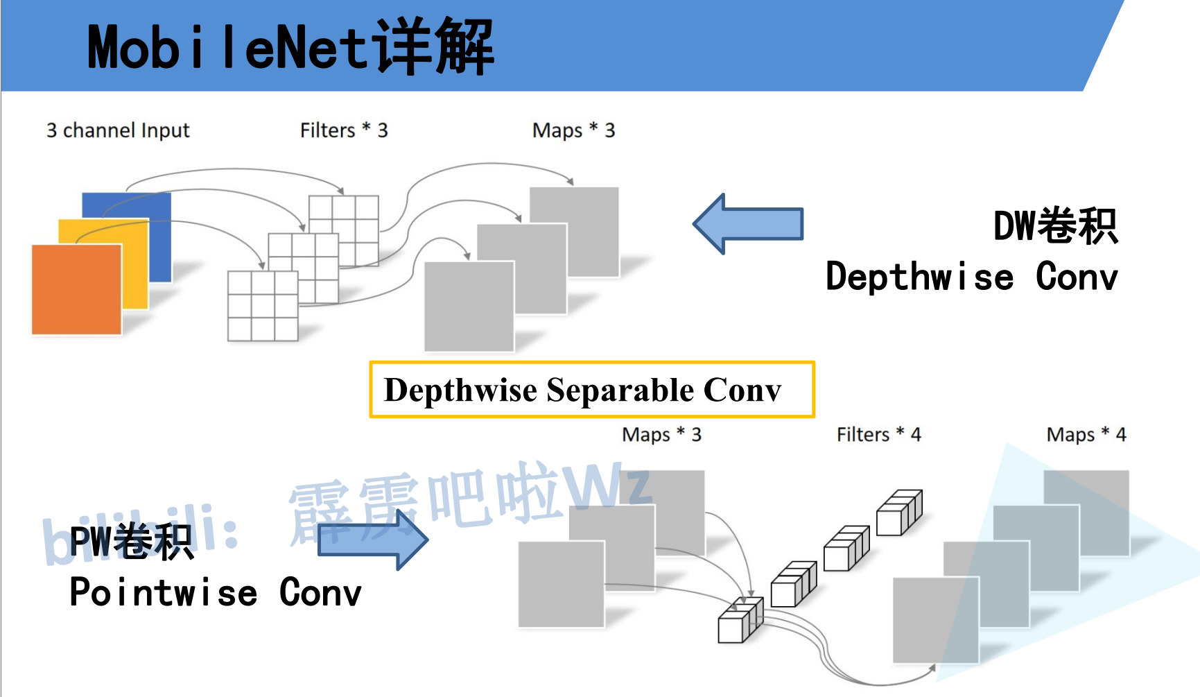
如上两个图，图中将这一过程清晰地分为上下两层：

第一步：深度卷积（DW）

输入：一张具有 3个通道​ 的输入图片（图中橙、黄、蓝三个方块）。

操作：使用 3个独立的卷积核（Filters * 3），每个核只负责处理一个对应的输入通道。图中用三个浅灰色网格表示。

输出：生成 3个特征图（Maps * 3）。每个特征图是单一通道的，其信息仅来源于对应的输入通道。

本质：这是在二维平面（高度、宽度）上进行卷积，完全忽略了通道间的信息交互。

第二步：逐点卷积（PW）

输入：深度卷积输出的 3个特征图。

操作：使用 4个1x1大小的卷积核（Filters * 4）对输入进行处理。1x1卷积的独特之处在于，它只混合通道信息，不改变特征图的空间尺寸。

输出：生成 4个新的特征图（Maps * 4）。

本质：这是在通道维度上进行线性组合，将上一步得到的各个通道的特征，以可学习的方式加权融合，以生成新的、具有特定语义的特征。

标准卷积的计算量

假设输入特征图大小为 D_F × D_F × M，使用 N 个 D_K × D_K 的卷积核，输出特征图大小为 D_F × D_F × N：

标准卷积计算量 = D_K × D_K × M × N × D_F × D_F

深度可分离卷积的计算量

• Depthwise卷积：D_K × D_K × 1 × M × D_F × D_F（每个通道独立卷积）
• Pointwise卷积：1 × 1 × M × N × D_F × D_F（1x1卷积融合通道）

深度可分离卷积总计算量 = D_K × D_K × M × D_F × D_F + M × N × D_F × D_F

计算量比值

深度可分离卷积 / 标准卷积 = (D_K × D_K × M × D_F × D_F + M × N × D_F × D_F) / (D_K × D_K × M × N × D_F × D_F)
= 1/N + 1/D_K²

当使用3×3卷积核时：

1/N + 1/9 ≈ 1/8 ~ 1/9

也就是说，深度可分离卷积的计算量仅为标准卷积的1/8到1/9，而准确率仅有极小的下降！

1.3 宽度乘子α和分辨率乘子ρ

MobileNetV1还引入了两个超参数来进一步控制模型大小：

• 宽度乘子α（Width Multiplier）：统一缩放每层的通道数。α=1为标准MobileNet，α<1为缩小版（如0.75、0.5、0.25）
• 分辨率乘子ρ（Resolution Multiplier）：统一缩放输入图像和每层特征图的空间分辨率

引入α后，计算量变为：

D_K × D_K × αM × ρD_F × ρD_F + αM × αN × ρD_F × ρD_F

1.4 V1的缺陷

MobileNetV1存在一个明显的问题：Depthwise卷积的输出通道数等于输入通道数，无法改变通道维度，导致信息表达能力受限。同时，Depthwise部分的卷积核容易训练到接近0，导致部分"死亡"。

---

二、MobileNetV2

2.1 MobileNetV2介绍

MobileNetV2在2018年提出，在V1的基础上做出了关键改进。论文标题中的"Inverted Residuals"和"Linear Bottlenecks"就是两大核心创新。

网络中的亮点：

1. Inverted Residual（倒残差结构）：与传统残差结构"两头大中间小"相反，倒残差结构是"两头小中间大"
2. Linear Bottleneck（线性瓶颈）：最后的1x1卷积后不使用ReLU激活函数，改用线性输出

2.2 倒残差结构（Inverted Residual）

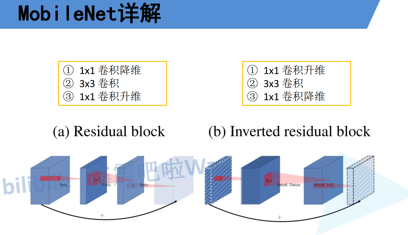
对比ResNet的残差结构和MobileNetV2的倒残差结构：

	ResNet残差结构	MobileNetV2倒残差结构
结构	1×1降维 → 3×3卷积 → 1×1升维	1×1升维 → 3×3 DW卷积 → 1×1降维
形状	大 → 小 → 大	小 → 大 → 小
激活	ReLU → ReLU → ReLU	ReLU6 → ReLU6 → 线性（无激活）
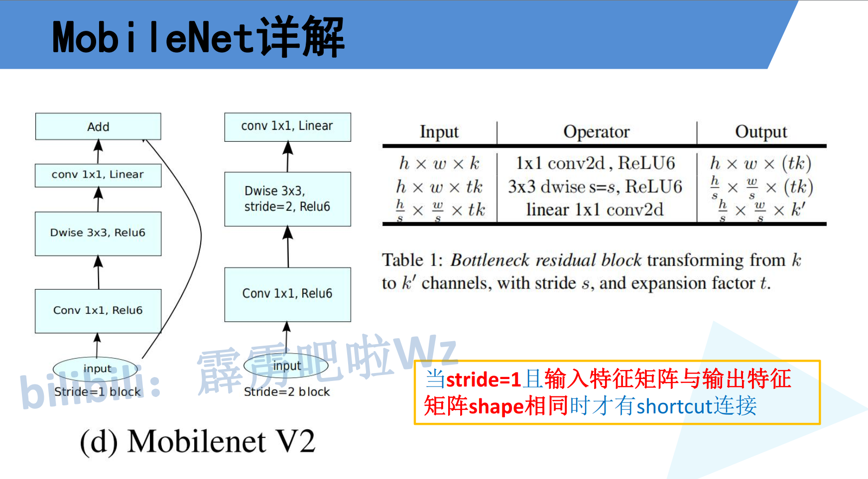
连接	恒等映射	恒等映射（仅stride=1且输入输出通道相同时）

倒残差结构的工作流程：

1. Expand（扩展）：1×1卷积将低维空间映射到高维空间（乘以扩展因子t）
2. Depthwise（深度卷积）：3×3深度可分离卷积在高维空间中提取特征
3. Project（投影）：1×1卷积将高维空间投影回低维空间（无ReLU激活）

2.3 为什么用ReLU6？

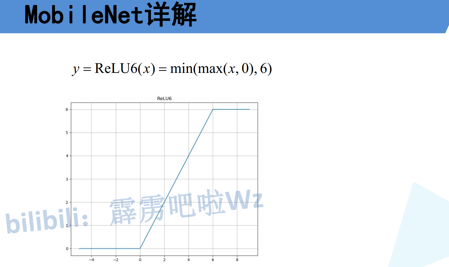
ReLU6的数学表达式为：min(max(x, 0), 6)，即输出被截断在[0, 6]之间。

在移动端部署时，ReLU6的最大输出值为6，便于用8位（int8）定点数表示（6/255 ≈ 0.024，精度足够），避免了ReLU无上界导致的量化精度损失。

2.4 为什么最后一层不用ReLU？（Linear Bottleneck）

ReLU激活函数对低维特征会造成严重的信息丢失：

• 如果输入的低维流形恰好位于高维空间的某个象限内，经过ReLU后信息被保留
• 但如果低维流形跨越多个象限，经过ReLU后整个维度上的信息可能完全丢失
• 而在倒残差结构的最后一层（Project层），输出已经是低维的，如果再用ReLU激活，信息损失会非常严重

因此，MobileNetV2在最后的1×1卷积（Project层）后使用线性激活（即不使用激活函数），以保留低维空间中的完整信息。

2.5 MobileNetV2网络结构

MobileNetV2的整体结构参数表：

输入尺寸	算子	t（扩展因子）	c（输出通道）	n（重复次数）	s（步长）
224²×3	Conv2d 3×3	-	32	1	2
112²×32	Bottleneck	1	16	1	1
112²×16	Bottleneck	6	24	2	2
56²×24	Bottleneck	6	32	3	2
28²×32	Bottleneck	6	64	4	2
14²×64	Bottleneck	6	96	3	1
14²×96	Bottleneck	6	160	3	2
7²×160	Bottleneck	6	320	1	1
7²×320	Conv2d 1×1	-	1280	1	1
7²×1280	AvgPool 7×7	-	-	1	-
1²×1280	FC	-	k	-	-

其中t=1的第一行Bottleneck没有扩展步骤，直接进行深度卷积

注意：只有stride=1且输入通道等于输出通道时，才使用残差连接（shortcut）。

---

三、MobileNetV3

3.1 MobileNetV3介绍

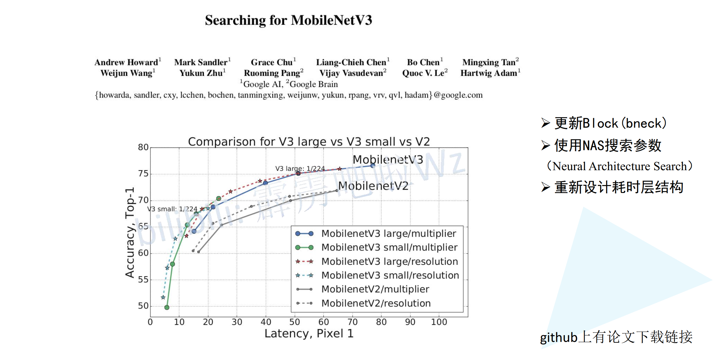
MobileNetV3在2019年提出，与前两代由人工设计不同，V3大量使用了**NAS（网络结构搜索）**技术。论文通过组合MnasNet和NetAdapt两种搜索策略来自动寻找最优网络结构。

网络中的亮点：

1. NAS搜索网络结构：不再完全由人工设计
2. 引入SE（Squeeze-and-Excitation）注意力模块
3. 使用h-swish和h-sigmoid激活函数替代部分ReLU和sigmoid
4. 提供Large和Small两个版本，适应不同算力需求
5. 重新设计网络尾部结构，进一步减少计算量

3.2 激活函数的改进

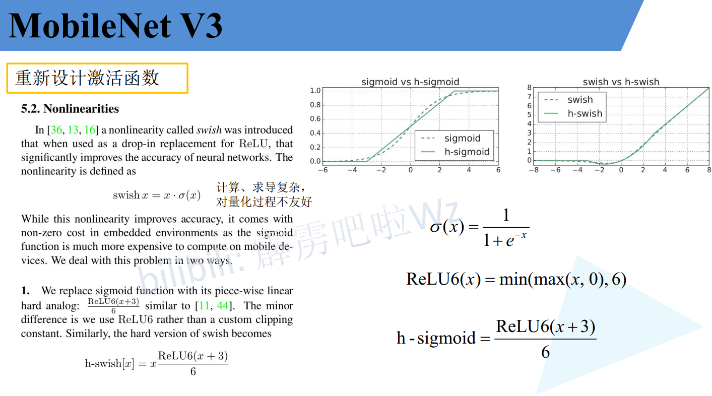
Swish激活函数

swish(x) = x × σ(x)，其中σ(x)为sigmoid函数

Swish激活函数被Google研究发现能提升模型精度，但sigmoid计算代价较高。

h-swish（hard swish）

h-swish(x) = x × h-sigmoid(x) / 6

其中 h-sigmoid(x) = min(max(x + 3, 0), 6)

h-swish是swish的分段线性近似，计算更快，且在量化部署时更友好。

注意：并不是网络中所有层都使用h-swish。在MobileNetV3中，只有较深层的Bottleneck使用h-swish（表中标记为"HS"），浅层仍然使用ReLU6（标记为"RE"）。这是因为h-swish在低维空间中的增益不明显，且计算开销更大。

3.3 SE注意力模块

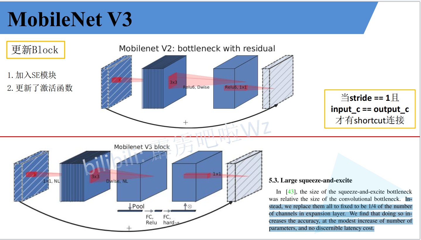
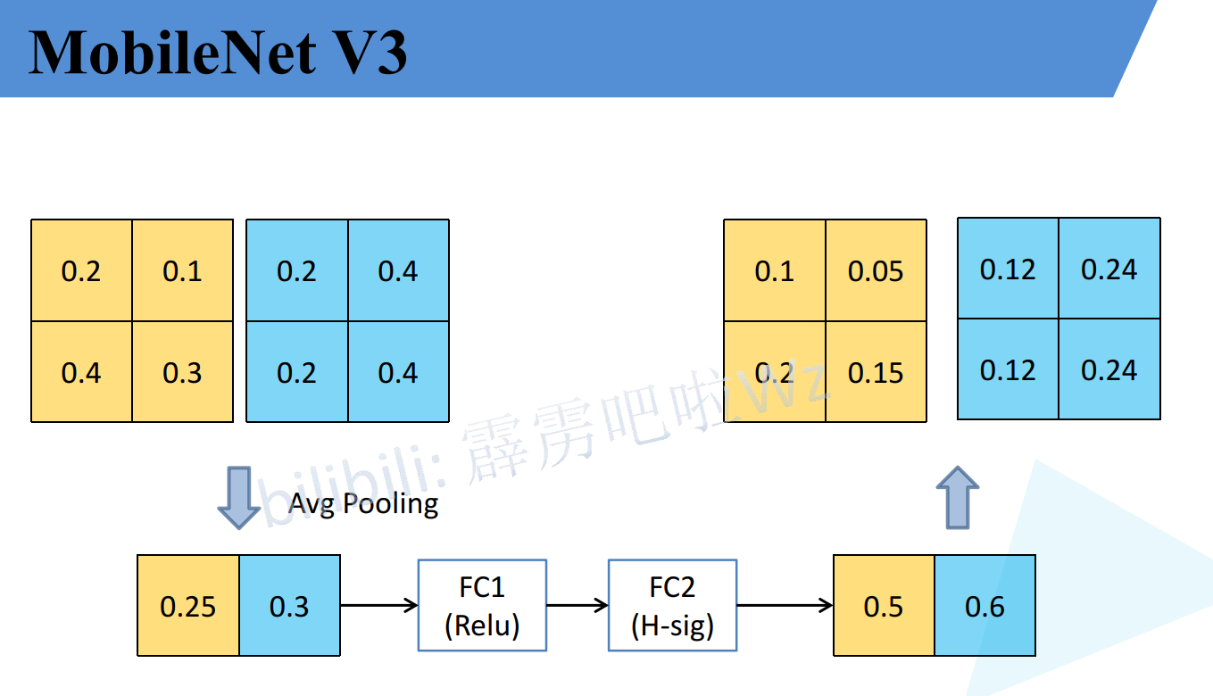
SE（Squeeze-and-Excitation）模块的核心思想是对通道维度进行注意力加权：

1. Squeeze（压缩）：通过全局平均池化将每个通道压缩为一个标量，得到1×1×C的向量
2. Excitation（激励）：通过两个全连接层（先降维再升维）学习每个通道的重要性权重
3. Scale（缩放）：将学到的权重乘回原特征图

在MobileNetV3中，SE模块放置在深度卷积之后、逐点卷积之前：

1×1扩展 → 3×3 DW卷积 → SE模块 → 1×1投影

SE模块的参数：降维比例默认为1/4，即全连接层先将通道数压缩为1/4，再恢复回原通道数。

3.4 耗时层结构改进

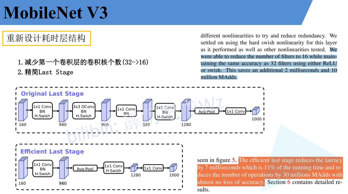
1、减少第一个卷积层的卷积核个数：从 32 个减少到 16 个。

2、精简最后的特征提取阶段：对 “Last Stage” 进行重构和简化。

3.5 MobileNetV3-Large网络结构

输入通道	卷积核	扩展通道	输出通道	SE	激活	步长
16	3	16	16	✗	RE	1
16	3	64	24	✗	RE	2
24	3	72	24	✗	RE	1
24	5	72	40	✓	RE	2
40	5	120	40	✓	RE	1
40	5	120	40	✓	RE	1
40	3	240	80	✗	HS	2
80	3	200	80	✗	HS	1
80	3	184	80	✗	HS	1
80	3	184	80	✗	HS	1
80	3	480	112	✓	HS	1
112	3	672	112	✓	HS	1
112	5	672	160	✓	HS	2
160	5	960	160	✓	HS	1
160	5	960	160	✓	HS	1

"RE"表示ReLU6，"HS"表示h-swish。注意从第7行开始激活函数从RE切换为HS。

3.6 MobileNetV3-Small网络结构

输入通道	卷积核	扩展通道	输出通道	SE	激活	步长
16	3	16	16	✓	RE	2
16	3	72	24	✗	RE	2
24	3	88	24	✗	RE	1
24	5	96	40	✓	HS	2
40	5	240	40	✓	HS	1
40	5	240	40	✓	HS	1
40	5	120	48	✓	HS	1
48	5	144	48	✓	HS	1
48	5	288	96	✓	HS	2
96	5	576	96	✓	HS	1
96	5	576	96	✓	HS	1

Small版本中SE模块使用更频繁，且更早切换到h-swish激活函数。

---

四、代码分析

4.1 model_v2.py（MobileNetV2）

from torch import nn
import torch


def _make_divisible(ch, divisor=8, min_ch=None):
    """
    This function is taken from the original tf repo.
    It ensures that all layers have a channel number that is divisible by 8
    It can be seen here:
    https://github.com/tensorflow/models/blob/master/research/slim/nets/mobilenet/mobilenet.py
    """
    if min_ch is None:
        min_ch = divisor
    new_ch = max(min_ch, int(ch + divisor / 2) // divisor * divisor)
    # Make sure that round down does not go down by more than 10%.
    if new_ch < 0.9 * ch:
        new_ch += divisor
    return new_ch


class ConvBNReLU(nn.Sequential):
    def __init__(self, in_channel, out_channel, kernel_size=3, stride=1, groups=1):
        padding = (kernel_size - 1) // 2
        super(ConvBNReLU, self).__init__(
            nn.Conv2d(in_channel, out_channel, kernel_size, stride, padding, groups=groups, bias=False),
            nn.BatchNorm2d(out_channel),
            nn.ReLU6(inplace=True)
        )


class InvertedResidual(nn.Module):
    def __init__(self, in_channel, out_channel, stride, expand_ratio):
        super(InvertedResidual, self).__init__()
        hidden_channel = in_channel * expand_ratio
        self.use_shortcut = stride == 1 and in_channel == out_channel

        layers = []
        if expand_ratio != 1:
            # 1x1 pointwise conv
            layers.append(ConvBNReLU(in_channel, hidden_channel, kernel_size=1))
        layers.extend([
            # 3x3 depthwise conv
            ConvBNReLU(hidden_channel, hidden_channel, stride=stride, groups=hidden_channel),
            # 1x1 pointwise conv(linear)
            nn.Conv2d(hidden_channel, out_channel, kernel_size=1, bias=False),
            nn.BatchNorm2d(out_channel),
        ])

        self.conv = nn.Sequential(*layers)

    def forward(self, x):
        if self.use_shortcut:
            return x + self.conv(x)
        else:
            return self.conv(x)


class MobileNetV2(nn.Module):
    def __init__(self, num_classes=1000, alpha=1.0, round_nearest=8):
        super(MobileNetV2, self).__init__()
        block = InvertedResidual
        input_channel = _make_divisible(32 * alpha, round_nearest)
        last_channel = _make_divisible(1280 * alpha, round_nearest)

        inverted_residual_setting = [
            # t, c, n, s
            [1, 16, 1, 1],
            [6, 24, 2, 2],
            [6, 32, 3, 2],
            [6, 64, 4, 2],
            [6, 96, 3, 1],
            [6, 160, 3, 2],
            [6, 320, 1, 1],
        ]

        features = []
        # conv1 layer
        features.append(ConvBNReLU(3, input_channel, stride=2))
        # building inverted residual residual blockes
        for t, c, n, s in inverted_residual_setting:
            output_channel = _make_divisible(c * alpha, round_nearest)
            for i in range(n):
                stride = s if i == 0 else 1
                features.append(block(input_channel, output_channel, stride, expand_ratio=t))
                input_channel = output_channel
        # building last several layers
        features.append(ConvBNReLU(input_channel, last_channel, 1))
        # combine feature layers
        self.features = nn.Sequential(*features)

        # building classifier
        self.avgpool = nn.AdaptiveAvgPool2d((1, 1))
        self.classifier = nn.Sequential(
            nn.Dropout(0.2),
            nn.Linear(last_channel, num_classes)
        )

        # weight initialization
        for m in self.modules():
            if isinstance(m, nn.Conv2d):
                nn.init.kaiming_normal_(m.weight, mode='fan_out')
                if m.bias is not None:
                    nn.init.zeros_(m.bias)
            elif isinstance(m, nn.BatchNorm2d):
                nn.init.ones_(m.weight)
                nn.init.zeros_(m.bias)
            elif isinstance(m, nn.Linear):
                nn.init.normal_(m.weight, 0, 0.01)
                nn.init.zeros_(m.bias)

    def forward(self, x):
        x = self.features(x)
        x = self.avgpool(x)
        x = torch.flatten(x, 1)
        x = self.classifier(x)
        return x

代码解析：

_make_divisible函数

这个函数的作用是确保通道数能被divisor（默认8）整除。这是为了适配硬件加速器（如NPU、DSP），这些硬件通常在通道数为8的倍数时运算效率最高。同时，函数保证调整后的通道数与原始值的偏差不超过10%，避免信息损失过大。

ConvBNReLU类

将"卷积 + BN + ReLU6"封装为一个模块，继承自nn.Sequential。注意这里统一使用ReLU6而非ReLU。groups=1为默认的标准卷积，当groups=in_channel时则为深度卷积。

InvertedResidual类（倒残差结构）

这是MobileNetV2的核心模块，需要重点关注几个细节：

1. self.use_shortcut：只有stride=1且输入输出通道相同时才使用残差连接。与ResNet的残差连接条件一致。

2. expand_ratio != 1时才添加1×1扩展层：当扩展因子为1时，扩展后的通道数等于输入通道数，无需扩展。对应网络结构表中第一行t=1的情况。

3. 最后一层1×1卷积后没有ReLU：代码中nn.Conv2d(hidden_channel, out_channel, kernel_size=1, bias=False)后只接了BN，没有ReLU6，这就是Linear Bottleneck的实现。前面扩展和深度卷积使用ConvBNReLU（含ReLU6），而最后的投影层直接Conv2d + BN，无激活函数。

4. 深度卷积的groups=hidden_channel：PyTorch中groups参数等于输入通道数时，就是深度卷积——每个通道独立卷积。

MobileNetV2主类

• alpha参数：宽度乘子，缩放每层通道数。alpha<1时模型更小更快
• inverted_residual_setting：列表中每行 [t, c, n, s] 分别表示扩展因子、输出通道、重复次数、步长
• 每个t/c/n/s组中，只有第一个block使用stride=s，其余使用stride=1：通过stride = s if i == 0 else 1实现
• 分类器非常简单：Dropout + 全连接，没有额外的全连接层

---

4.2 model_v3.py（MobileNetV3）

from typing import Callable, List, Optional

import torch
from torch import nn, Tensor
from torch.nn import functional as F
from functools import partial


def _make_divisible(ch, divisor=8, min_ch=None):
    """
    This function is taken from the original tf repo.
    It ensures that all layers have a channel number that is divisible by 8
    It can be seen here:
    https://github.com/tensorflow/models/blob/master/research/slim/nets/mobilenet/mobilenet.py
    """
    if min_ch is None:
        min_ch = divisor
    new_ch = max(min_ch, int(ch + divisor / 2) // divisor * divisor)
    # Make sure that round down does not go down by more than 10%.
    if new_ch < 0.9 * ch:
        new_ch += divisor
    return new_ch


class ConvBNActivation(nn.Sequential):
    def __init__(self,
                 in_planes: int,
                 out_planes: int,
                 kernel_size: int = 3,
                 stride: int = 1,
                 groups: int = 1,
                 norm_layer: Optional[Callable[..., nn.Module]] = None,
                 activation_layer: Optional[Callable[..., nn.Module]] = None):
        padding = (kernel_size - 1) // 2
        if norm_layer is None:
            norm_layer = nn.BatchNorm2d
        if activation_layer is None:
            activation_layer = nn.ReLU6
        super(ConvBNActivation, self).__init__(nn.Conv2d(in_channels=in_planes,
                                                         out_channels=out_planes,
                                                         kernel_size=kernel_size,
                                                         stride=stride,
                                                         padding=padding,
                                                         groups=groups,
                                                         bias=False),
                                               norm_layer(out_planes),
                                               activation_layer(inplace=True))


class SqueezeExcitation(nn.Module):
    def __init__(self, input_c: int, squeeze_factor: int = 4):
        super(SqueezeExcitation, self).__init__()
        squeeze_c = _make_divisible(input_c // squeeze_factor, 8)
        self.fc1 = nn.Conv2d(input_c, squeeze_c, 1)
        self.fc2 = nn.Conv2d(squeeze_c, input_c, 1)

    def forward(self, x: Tensor) -> Tensor:
        scale = F.adaptive_avg_pool2d(x, output_size=(1, 1))
        scale = self.fc1(scale)
        scale = F.relu(scale, inplace=True)
        scale = self.fc2(scale)
        scale = F.hardsigmoid(scale, inplace=True)
        return scale * x


class InvertedResidualConfig:
    def __init__(self,
                 input_c: int,
                 kernel: int,
                 expanded_c: int,
                 out_c: int,
                 use_se: bool,
                 activation: str,
                 stride: int,
                 width_multi: float):
        self.input_c = self.adjust_channels(input_c, width_multi)
        self.kernel = kernel
        self.expanded_c = self.adjust_channels(expanded_c, width_multi)
        self.out_c = self.adjust_channels(out_c, width_multi)
        self.use_se = use_se
        self.use_hs = activation == "HS"  # whether using h-swish activation
        self.stride = stride

    @staticmethod
    def adjust_channels(channels: int, width_multi: float):
        return _make_divisible(channels * width_multi, 8)


class InvertedResidual(nn.Module):
    def __init__(self,
                 cnf: InvertedResidualConfig,
                 norm_layer: Callable[..., nn.Module]):
        super(InvertedResidual, self).__init__()

        if cnf.stride not in [1, 2]:
            raise ValueError("illegal stride value.")

        self.use_res_connect = (cnf.stride == 1 and cnf.input_c == cnf.out_c)

        layers: List[nn.Module] = []
        activation_layer = nn.Hardswish if cnf.use_hs else nn.ReLU

        # expand
        if cnf.expanded_c != cnf.input_c:
            layers.append(ConvBNActivation(cnf.input_c,
                                           cnf.expanded_c,
                                           kernel_size=1,
                                           norm_layer=norm_layer,
                                           activation_layer=activation_layer))

        # depthwise
        layers.append(ConvBNActivation(cnf.expanded_c,
                                       cnf.expanded_c,
                                       kernel_size=cnf.kernel,
                                       stride=cnf.stride,
                                       groups=cnf.expanded_c,
                                       norm_layer=norm_layer,
                                       activation_layer=activation_layer))

        if cnf.use_se:
            layers.append(SqueezeExcitation(cnf.expanded_c))

        # project
        layers.append(ConvBNActivation(cnf.expanded_c,
                                       cnf.out_c,
                                       kernel_size=1,
                                       norm_layer=norm_layer,
                                       activation_layer=nn.Identity))

        self.block = nn.Sequential(*layers)
        self.out_channels = cnf.out_c
        self.is_strided = cnf.stride > 1

    def forward(self, x: Tensor) -> Tensor:
        result = self.block(x)
        if self.use_res_connect:
            result += x

        return result


class MobileNetV3(nn.Module):
    def __init__(self,
                 inverted_residual_setting: List[InvertedResidualConfig],
                 last_channel: int,
                 num_classes: int = 1000,
                 block: Optional[Callable[..., nn.Module]] = None,
                 norm_layer: Optional[Callable[..., nn.Module]] = None):
        super(MobileNetV3, self).__init__()

        if not inverted_residual_setting:
            raise ValueError("The inverted_residual_setting should not be empty.")
        elif not (isinstance(inverted_residual_setting, List) and
                  all([isinstance(s, InvertedResidualConfig) for s in inverted_residual_setting])):
            raise TypeError("The inverted_residual_setting should be List[InvertedResidualConfig]")

        if block is None:
            block = InvertedResidual

        if norm_layer is None:
            norm_layer = partial(nn.BatchNorm2d, eps=0.001, momentum=0.01)

        layers: List[nn.Module] = []

        # building first layer
        firstconv_output_c = inverted_residual_setting[0].input_c
        layers.append(ConvBNActivation(3,
                                       firstconv_output_c,
                                       kernel_size=3,
                                       stride=2,
                                       norm_layer=norm_layer,
                                       activation_layer=nn.Hardswish))
        # building inverted residual blocks
        for cnf in inverted_residual_setting:
            layers.append(block(cnf, norm_layer))

        # building last several layers
        lastconv_input_c = inverted_residual_setting[-1].out_c
        lastconv_output_c = 6 * lastconv_input_c
        layers.append(ConvBNActivation(lastconv_input_c,
                                       lastconv_output_c,
                                       kernel_size=1,
                                       norm_layer=norm_layer,
                                       activation_layer=nn.Hardswish))
        self.features = nn.Sequential(*layers)
        self.avgpool = nn.AdaptiveAvgPool2d(1)
        self.classifier = nn.Sequential(nn.Linear(lastconv_output_c, last_channel),
                                        nn.Hardswish(inplace=True),
                                        nn.Dropout(p=0.2, inplace=True),
                                        nn.Linear(last_channel, num_classes))

        # initial weights
        for m in self.modules():
            if isinstance(m, nn.Conv2d):
                nn.init.kaiming_normal_(m.weight, mode="fan_out")
                if m.bias is not None:
                    nn.init.zeros_(m.bias)
            elif isinstance(m, (nn.BatchNorm2d, nn.GroupNorm)):
                nn.init.ones_(m.weight)
                nn.init.zeros_(m.bias)
            elif isinstance(m, nn.Linear):
                nn.init.normal_(m.weight, 0, 0.01)
                nn.init.zeros_(m.bias)

    def _forward_impl(self, x: Tensor) -> Tensor:
        x = self.features(x)
        x = self.avgpool(x)
        x = torch.flatten(x, 1)
        x = self.classifier(x)

        return x

    def forward(self, x: Tensor) -> Tensor:
        return self._forward_impl(x)


def mobilenet_v3_large(num_classes: int = 1000,
                       reduced_tail: bool = False) -> MobileNetV3:
    """
    Constructs a large MobileNetV3 architecture from
    "Searching for MobileNetV3" <https://arxiv.org/abs/1905.02244>.

    weights_link:
    https://download.pytorch.org/models/mobilenet_v3_large-8738ca79.pth

    Args:
        num_classes (int): number of classes
        reduced_tail (bool): If True, reduces the channel counts of all feature layers
            between C4 and C5 by 2. It is used to reduce the channel redundancy in the
            backbone for Detection and Segmentation.
    """
    width_multi = 1.0
    bneck_conf = partial(InvertedResidualConfig, width_multi=width_multi)
    adjust_channels = partial(InvertedResidualConfig.adjust_channels, width_multi=width_multi)

    reduce_divider = 2 if reduced_tail else 1

    inverted_residual_setting = [
        # input_c, kernel, expanded_c, out_c, use_se, activation, stride
        bneck_conf(16, 3, 16, 16, False, "RE", 1),
        bneck_conf(16, 3, 64, 24, False, "RE", 2),  # C1
        bneck_conf(24, 3, 72, 24, False, "RE", 1),
        bneck_conf(24, 5, 72, 40, True, "RE", 2),  # C2
        bneck_conf(40, 5, 120, 40, True, "RE", 1),
        bneck_conf(40, 5, 120, 40, True, "RE", 1),
        bneck_conf(40, 3, 240, 80, False, "HS", 2),  # C3
        bneck_conf(80, 3, 200, 80, False, "HS", 1),
        bneck_conf(80, 3, 184, 80, False, "HS", 1),
        bneck_conf(80, 3, 184, 80, False, "HS", 1),
        bneck_conf(80, 3, 480, 112, True, "HS", 1),
        bneck_conf(112, 3, 672, 112, True, "HS", 1),
        bneck_conf(112, 5, 672, 160 // reduce_divider, True, "HS", 2),  # C4
        bneck_conf(160 // reduce_divider, 5, 960 // reduce_divider, 160 // reduce_divider, True, "HS", 1),
        bneck_conf(160 // reduce_divider, 5, 960 // reduce_divider, 160 // reduce_divider, True, "HS", 1),
    ]
    last_channel = adjust_channels(1280 // reduce_divider)  # C5

    return MobileNetV3(inverted_residual_setting=inverted_residual_setting,
                       last_channel=last_channel,
                       num_classes=num_classes)


def mobilenet_v3_small(num_classes: int = 1000,
                       reduced_tail: bool = False) -> MobileNetV3:
    """
    Constructs a large MobileNetV3 architecture from
    "Searching for MobileNetV3" <https://arxiv.org/abs/1905.02244>.

    weights_link:
    https://download.pytorch.org/models/mobilenet_v3_small-047dcff4.pth

    Args:
        num_classes (int): number of classes
        reduced_tail (bool): If True, reduces the channel counts of all feature layers
            between C4 and C5 by 2. It is used to reduce the channel redundancy in the
            backbone for Detection and Segmentation.
    """
    width_multi = 1.0
    bneck_conf = partial(InvertedResidualConfig, width_multi=width_multi)
    adjust_channels = partial(InvertedResidualConfig.adjust_channels, width_multi=width_multi)

    reduce_divider = 2 if reduced_tail else 1

    inverted_residual_setting = [
        # input_c, kernel, expanded_c, out_c, use_se, activation, stride
        bneck_conf(16, 3, 16, 16, True, "RE", 2),  # C1
        bneck_conf(16, 3, 72, 24, False, "RE", 2),  # C2
        bneck_conf(24, 3, 88, 24, False, "RE", 1),
        bneck_conf(24, 5, 96, 40, True, "HS", 2),  # C3
        bneck_conf(40, 5, 240, 40, True, "HS", 1),
        bneck_conf(40, 5, 240, 40, True, "HS", 1),
        bneck_conf(40, 5, 120, 48, True, "HS", 1),
        bneck_conf(48, 5, 144, 48, True, "HS", 1),
        bneck_conf(48, 5, 288, 96 // reduce_divider, True, "HS", 2),  # C4
        bneck_conf(96 // reduce_divider, 5, 576 // reduce_divider, 96 // reduce_divider, True, "HS", 1),
        bneck_conf(96 // reduce_divider, 5, 576 // reduce_divider, 96 // reduce_divider, True, "HS", 1)
    ]
    last_channel = adjust_channels(1024 // reduce_divider)  # C5

    return MobileNetV3(inverted_residual_setting=inverted_residual_setting,
                       last_channel=last_channel,
                       num_classes=num_classes)

代码解析：

MobileNetV3的代码比V2复杂不少，主要体现在以下几个方面：

ConvBNActivation类

与V2的ConvBNReLU类似，但更加灵活——激活函数可以通过参数指定。V2固定使用ReLU6，V3可以根据配置选择ReLU、Hardswish或Identity（无激活）。这种设计使得同一个模块可以适配网络中不同位置的需求。

SqueezeExcitation类（SE注意力模块）

SE模块的实现非常简洁：

1. F.adaptive_avg_pool2d(x, output_size=(1, 1))：全局平均池化，Squeeze操作
2. self.fc1：1×1卷积降维（通道数压缩为1/4）
3. self.fc2：1×1卷积升维（恢复回原始通道数）
4. F.hardsigmoid：生成0~1之间的通道权重
5. scale * x：将权重乘回原特征图

注意SE模块中使用的是**1×1卷积（Conv2d）**而非全连接层（Linear），效果等价但在实现上更方便。

InvertedResidualConfig类

V3引入了配置类来管理每个Bottleneck的参数。与V2直接在列表中写 [t, c, n, s] 不同，V3为每个block都单独配置了：输入通道、卷积核大小、扩展通道、输出通道、是否使用SE、激活函数类型、步长。这是因为V3每个block的参数差异更大（不同kernel size、有的有SE有的没有、激活函数不同），用配置类更清晰。

配置类中的 adjust_channels 方法会根据 width_multi 对通道数进行缩放，并确保结果能被8整除。

InvertedResidual类（V3版）

与V2的倒残差结构相比，V3的InvertedResidual有以下不同：

1. 激活函数可选：nn.Hardswish if cnf.use_hs else nn.ReLU，不再是固定的ReLU6
2. 可选SE模块：if cnf.use_se: layers.append(SqueezeExcitation(cnf.expanded_c))
3. Project层使用nn.Identity：即无激活函数（Linear Bottleneck），与V2一致
4. 不再使用ReLU6：V3中ReLU和Hardswish替代了V2中的ReLU6

MobileNetV3主类

与V2相比的主要变化：

1. 首层卷积使用Hardswish：activation_layer=nn.Hardswish，V2首层用的是ReLU6
2. 分类器更复杂：
   • V2：Dropout → Linear
   • V3：Linear → Hardswish → Dropout → Linear
   • V3多了一个中间全连接层和Hardswish激活
3. lastconv_output_c = 6 * lastconv_input_c：最后一个1×1卷积将通道数扩展6倍，V2是扩展到固定的1280
4. reduced_tail参数：当用于检测和分割任务时，可以减半C4~C5之间的通道数，减少冗余

mobilenet_v3_large / mobilenet_v3_small

两个工厂函数分别创建Large和Small版本。注意使用partial简化配置创建：

bneck_conf = partial(InvertedResidualConfig, width_multi=width_multi)

这样每次调用 bneck_conf(16, 3, 16, 16, False, "RE", 1) 就自动传入了 width_multi，无需重复书写。

---

4.3 train.py

import os
import sys
import json

import torch
import torch.nn as nn
import torch.optim as optim
from torchvision import transforms, datasets
from tqdm import tqdm

from model_v2 import MobileNetV2


def main():
    device = torch.device("cuda:0" if torch.cuda.is_available() else "cpu")
    print("using {} device.".format(device))

    batch_size = 16
    epochs = 5

    data_transform = {
        "train": transforms.Compose([transforms.RandomResizedCrop(224),
                                     transforms.RandomHorizontalFlip(),
                                     transforms.ToTensor(),
                                     transforms.Normalize([0.485, 0.456, 0.406], [0.229, 0.224, 0.225])]),
        "val": transforms.Compose([transforms.Resize(256),
                                   transforms.CenterCrop(224),
                                   transforms.ToTensor(),
                                   transforms.Normalize([0.485, 0.456, 0.406], [0.229, 0.224, 0.225])])}

    data_root = os.path.abspath(os.path.join(os.getcwd(), "../.."))  # get data root path
    image_path = os.path.join(data_root, "data_set", "flower_data")  # flower data set path
    assert os.path.exists(image_path), "{} path does not exist.".format(image_path)
    train_dataset = datasets.ImageFolder(root=os.path.join(image_path, "train"),
                                         transform=data_transform["train"])
    train_num = len(train_dataset)

    # {'daisy':0, 'dandelion':1, 'roses':2, 'sunflower':3, 'tulips':4}
    flower_list = train_dataset.class_to_idx
    cla_dict = dict((val, key) for key, val in flower_list.items())
    # write dict into json file
    json_str = json.dumps(cla_dict, indent=4)
    with open('class_indices.json', 'w') as json_file:
        json_file.write(json_str)

    nw = min([os.cpu_count(), batch_size if batch_size > 1 else 0, 8])  # number of workers
    print('Using {} dataloader workers every process'.format(nw))

    train_loader = torch.utils.data.DataLoader(train_dataset,
                                               batch_size=batch_size, shuffle=True,
                                               num_workers=nw)

    validate_dataset = datasets.ImageFolder(root=os.path.join(image_path, "val"),
                                            transform=data_transform["val"])
    val_num = len(validate_dataset)
    validate_loader = torch.utils.data.DataLoader(validate_dataset,
                                                  batch_size=batch_size, shuffle=False,
                                                  num_workers=nw)

    print("using {} images for training, {} images for validation.".format(train_num,
                                                                           val_num))

    # create model
    net = MobileNetV2(num_classes=5)

    # load pretrain weights
    # download url: https://download.pytorch.org/models/mobilenet_v2-b0353104.pth
    model_weight_path = "./mobilenet_v2.pth"
    assert os.path.exists(model_weight_path), "file {} dose not exist.".format(model_weight_path)
    pre_weights = torch.load(model_weight_path, map_location='cpu')

    # delete classifier weights
    pre_dict = {k: v for k, v in pre_weights.items() if net.state_dict()[k].numel() == v.numel()}
    missing_keys, unexpected_keys = net.load_state_dict(pre_dict, strict=False)

    # freeze features weights
    for param in net.features.parameters():
        param.requires_grad = False

    net.to(device)

    # define loss function
    loss_function = nn.CrossEntropyLoss()

    # construct an optimizer
    params = [p for p in net.parameters() if p.requires_grad]
    optimizer = optim.Adam(params, lr=0.0001)

    best_acc = 0.0
    save_path = './MobileNetV2.pth'
    train_steps = len(train_loader)
    for epoch in range(epochs):
        # train
        net.train()
        running_loss = 0.0
        train_bar = tqdm(train_loader, file=sys.stdout)
        for step, data in enumerate(train_bar):
            images, labels = data
            optimizer.zero_grad()
            logits = net(images.to(device))
            loss = loss_function(logits, labels.to(device))
            loss.backward()
            optimizer.step()

            # print statistics
            running_loss += loss.item()

            train_bar.desc = "train epoch[{}/{}] loss:{:.3f}".format(epoch + 1,
                                                                     epochs,
                                                                     loss)

        # validate
        net.eval()
        acc = 0.0  # accumulate accurate number / epoch
        with torch.no_grad():
            val_bar = tqdm(validate_loader, file=sys.stdout)
            for val_data in val_bar:
                val_images, val_labels = val_data
                outputs = net(val_images.to(device))
                # loss = loss_function(outputs, test_labels)
                predict_y = torch.max(outputs, dim=1)[1]
                acc += torch.eq(predict_y, val_labels.to(device)).sum().item()

                val_bar.desc = "valid epoch[{}/{}]".format(epoch + 1,
                                                           epochs)
        val_accurate = acc / val_num
        print('[epoch %d] train_loss: %.3f  val_accuracy: %.3f' %
              (epoch + 1, running_loss / train_steps, val_accurate))

        if val_accurate > best_acc:
            best_acc = val_accurate
            torch.save(net.state_dict(), save_path)

    print('Finished Training')


if __name__ == '__main__':
    main()

代码解析：

train.py的整体框架与之前网络的训练脚本一致，但有几个重要区别：

1. 迁移学习的加载方式不同：

pre_dict = {k: v for k, v in pre_weights.items() if net.state_dict()[k].numel() == v.numel()}
missing_keys, unexpected_keys = net.load_state_dict(pre_dict, strict=False)

这里使用了一个巧妙的方法：通过 numel() 比较预训练权重和当前模型权重的元素个数。因为预训练模型是1000类的，而当前任务是5类，分类器最后一层的形状不同。元素个数不同的权重会被自动跳过，只加载匹配的权重。这比之前ResNet中手动删除fc层权重的方法更加优雅。

2. 冻结特征提取层：

for param in net.features.parameters():
    param.requires_grad = False

将features部分的所有参数设为不可训练，只训练分类器部分。这在迁移学习中很常见——预训练的特征提取器已经学到了通用特征，只需微调分类头即可。

3. 数据预处理使用ImageNet标准均值和标准差：

transforms.Normalize([0.485, 0.456, 0.406], [0.229, 0.224, 0.225])

与之前VGG/GoogLeNet代码中使用的 (0.5, 0.5, 0.5) 不同，这里使用的是ImageNet数据集的真实均值和标准差。这是因为使用了预训练权重，必须与预训练时的归一化方式保持一致。

---

4.4 predict.py

import os
import json

import torch
from PIL import Image
from torchvision import transforms
import matplotlib.pyplot as plt

from model_v2 import MobileNetV2


def main():
    device = torch.device("cuda:0" if torch.cuda.is_available() else "cpu")

    data_transform = transforms.Compose(
        [transforms.Resize(256),
         transforms.CenterCrop(224),
         transforms.ToTensor(),
         transforms.Normalize([0.485, 0.456, 0.406], [0.229, 0.224, 0.225])])

    # load image
    img_path = "../tulip.jpg"
    assert os.path.exists(img_path), "file: '{}' dose not exist.".format(img_path)
    img = Image.open(img_path)
    plt.imshow(img)
    # [N, C, H, W]
    img = data_transform(img)
    # expand batch dimension
    img = torch.unsqueeze(img, dim=0)

    # read class_indict
    json_path = './class_indices.json'
    assert os.path.exists(json_path), "file: '{}' dose not exist.".format(json_path)

    with open(json_path, "r") as f:
        class_indict = json.load(f)

    # create model
    model = MobileNetV2(num_classes=5).to(device)
    # load model weights
    model_weight_path = "./MobileNetV2.pth"
    model.load_state_dict(torch.load(model_weight_path, map_location=device))
    model.eval()
    with torch.no_grad():
        # predict class
        output = torch.squeeze(model(img.to(device))).cpu()
        predict = torch.softmax(output, dim=0)
        predict_cla = torch.argmax(predict).numpy()

    print_res = "class: {}   prob: {:.3}".format(class_indict[str(predict_cla)],
                                                 predict[predict_cla].numpy())
    plt.title(print_res)
    for i in range(len(predict)):
        print("class: {:10}   prob: {:.3}".format(class_indict[str(i)],
                                                  predict[i].numpy()))
    plt.show()


if __name__ == '__main__':
    main()

代码解析：

predict.py与之前网络的预测脚本结构一致，没有特殊差异。注意验证阶段的数据预处理同样使用了ImageNet标准归一化参数。

---

总结

MobileNet系列是轻量级网络的代表，从V1到V3的演进脉络非常清晰：

• MobileNetV1：提出深度可分离卷积，将标准卷积拆分为Depthwise + Pointwise，计算量降为约1/8
• MobileNetV2：引入倒残差结构（先升维再降维）和Linear Bottleneck（投影层不使用ReLU），解决了V1中Depthwise卷积信息表达能力弱的问题
• MobileNetV3：结合NAS自动搜索网络结构，引入SE注意力模块和h-swish激活函数，提供Large/Small两种配置

三个版本的设计哲学一脉相承——用最少的计算量获得尽可能高的精度，使得深度学习模型能够在手机、IoT设备等算力受限的平台上高效运行。

以上就是今天要讲的内容