【个人CNN学习记录之ResNet网络】

---

---

前言

在日常工作中，我专注于并行计算领域，主要依托GPGPU、NPU等高算力芯片进行开发。当前，高算力与AI已深度融合，计算与人工智能二者相辅相成：底层计算为实现通用算法与算子提供基础，而AI模型则能反哺并优化传统算法的决策效率与性能。为系统构建这方面的知识体系，我在公司导师的推荐下，跟随up主“霹雳吧啦Wz”的CNN系列视频进行学习，并通过博客记录学习过程，融入自己的理解与总结。

---

一、ResNet简介

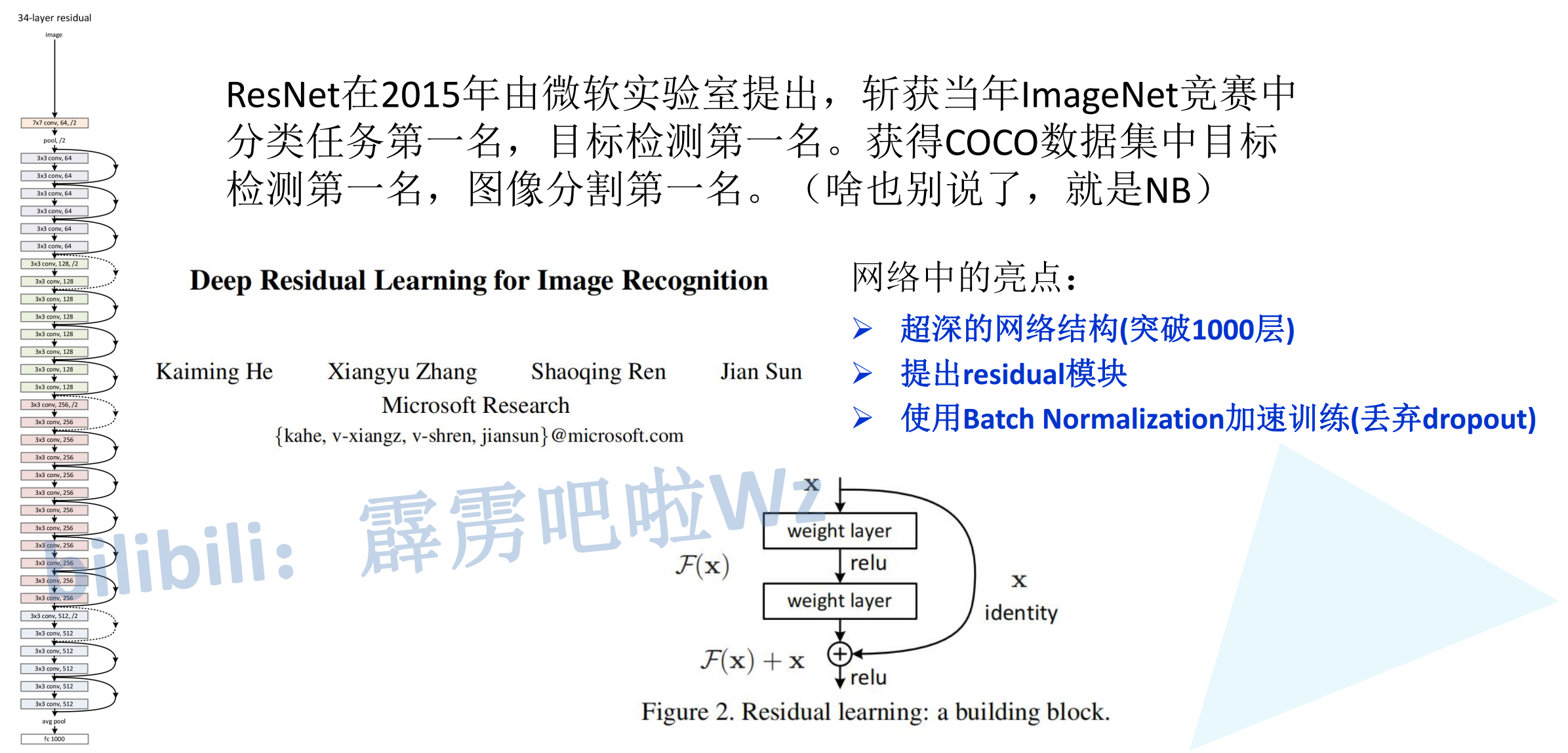
ResNet(Residual Network，残差网络)是2015年ILSVRC(ImageNet Large Scale Visual Recognition Challenge)分类任务的冠军网络，由微软研究院的何恺明等人提出。该网络以152层的超深网络结构取得了top-5错误率3.57%的惊人成绩，首次在ImageNet分类任务上超越了人类水平(约5%错误率)。ResNet的核心创新在于提出了残差学习(Residual Learning)，通过引入跳跃连接(Skip Connection)解决了深度网络训练中的梯度消失和退化问题。

1.1 问题背景

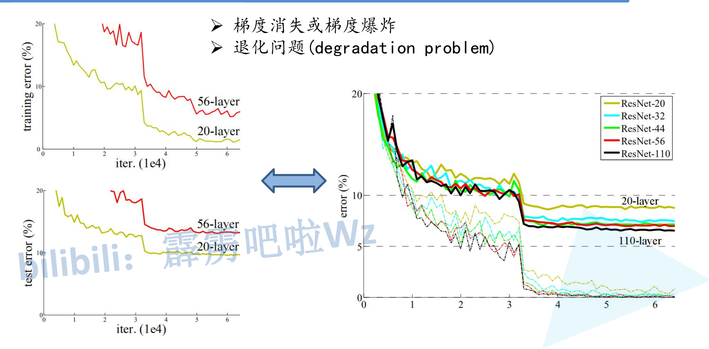
随着网络深度的增加，理论上网络应该能够提取更丰富的特征，获得更好的性能。然而实验发现：

1. 梯度消失/梯度爆炸：深层网络中反向传播时梯度会变得非常小或非常大，导致无法有效训练
2. 网络退化问题(Degradation Problem)：即使解决了梯度问题，深层网络的训练误差反而比浅层网络更高

1.2 退化问题分析

假设有一个浅层网络，在其后面添加更多层得到深层网络。理论上，新增的层可以学习恒等映射(Identity Mapping)，使得深层网络至少不会比浅层网络差。但实际上，直接训练深层网络往往难以学到恒等映射，导致性能下降。

这表明：现有的训练方法难以让深层网络很好地学习恒等映射。

---

二、残差学习

2.1 核心思想

ResNet提出了一种解决方案：与其让网络直接学习目标映射 H(x)，不如让网络学习残差映射 F(x) = H(x) - x，然后通过跳跃连接将输入 x 加到输出上，得到 H(x) = F(x) + x。
优势分析：

• 如果恒等映射是最优解，则只需让 F(x) = 0，这比直接学习 H(x) = x 容易得多
• 跳跃连接可以让梯度直接反向传播到浅层，缓解梯度消失问题
• 残差学习不增加额外参数和计算量

2.2 残差块结构

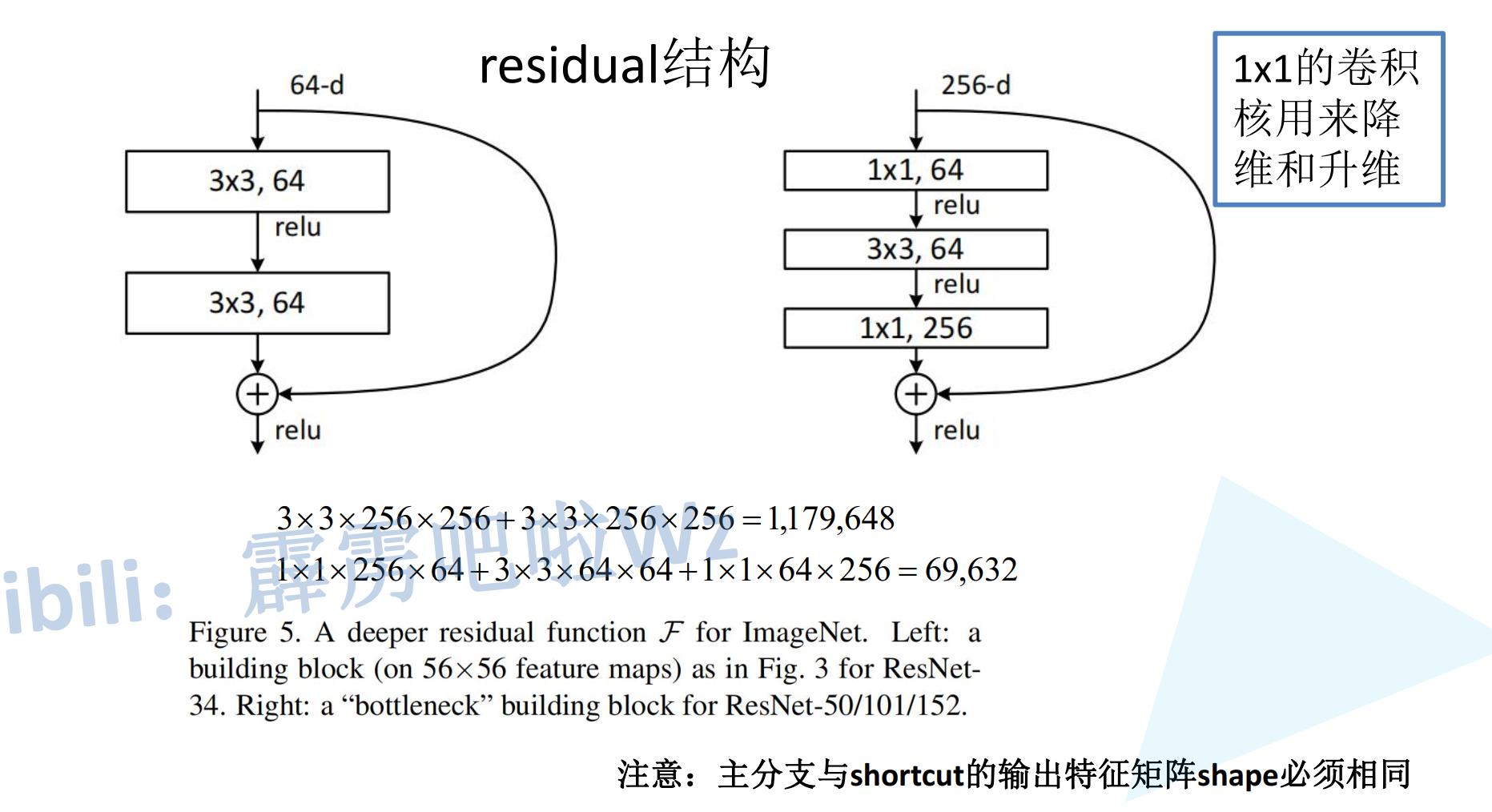
ResNet中有两种基本的残差块结构：

2.2.1 BasicBlock（用于ResNet-18/34）

BasicBlock由两个3×3卷积组成，适用于较浅的网络：

实线残差结构：输入输出通道数相同，可直接相加

虚线残差结构：输入输出通道数不同或需要下采样时，通过1×1卷积调整维度

class BasicBlock(nn.Module):
    expansion = 1  # 输出通道扩展倍数

    def __init__(self, in_channel, out_channel, stride=1, downsample=None, **kwargs):
        super(BasicBlock, self).__init__()
        self.conv1 = nn.Conv2d(in_channels=in_channel, out_channels=out_channel,
                               kernel_size=3, stride=stride, padding=1, bias=False)
        self.bn1 = nn.BatchNorm2d(out_channel)
        self.relu = nn.ReLU()
        self.conv2 = nn.Conv2d(in_channels=out_channel, out_channels=out_channel,
                               kernel_size=3, stride=1, padding=1, bias=False)
        self.bn2 = nn.BatchNorm2d(out_channel)
        self.downsample = downsample  # 维度调整分支

    def forward(self, x):
        identity = x
        if self.downsample is not None:
            identity = self.downsample(x)  # 调整维度以匹配输出

        out = self.conv1(x)
        out = self.bn1(out)
        out = self.relu(out)

        out = self.conv2(out)
        out = self.bn2(out)

        out += identity  # 残差连接
        out = self.relu(out)

        return out

2.2.2 Bottleneck（用于ResNet-50/101/152）

Bottleneck采用"瓶颈"结构，由1×1、3×3、1×1三个卷积组成，适用于深层网络：

设计思想：

• 第一个1×1卷积：降维，减少通道数
• 3×3卷积：在低维空间进行特征提取
• 最后一个1×1卷积：升维，恢复通道数

这种设计大大减少了参数量和计算量。

注意：PyTorch官方实现与原论文略有不同：

• 原论文：第一个1×1卷积stride=2，3×3卷积stride=1
• PyTorch实现：第一个1×1卷积stride=1，3×3卷积stride=2

这样做可以提升约0.5%的top-1准确率（ResNet v1.5）。

class Bottleneck(nn.Module):
    expansion = 4  # 输出通道扩展倍数

    def __init__(self, in_channel, out_channel, stride=1, downsample=None,
                 groups=1, width_per_group=64):
        super(Bottleneck, self).__init__()

        width = int(out_channel * (width_per_group / 64.)) * groups

        # 1x1卷积：降维
        self.conv1 = nn.Conv2d(in_channels=in_channel, out_channels=width,
                               kernel_size=1, stride=1, bias=False)
        self.bn1 = nn.BatchNorm2d(width)

        # 3x3卷积：特征提取
        self.conv2 = nn.Conv2d(in_channels=width, out_channels=width, groups=groups,
                               kernel_size=3, stride=stride, bias=False, padding=1)
        self.bn2 = nn.BatchNorm2d(width)

        # 1x1卷积：升维
        self.conv3 = nn.Conv2d(in_channels=width, out_channels=out_channel*self.expansion,
                               kernel_size=1, stride=1, bias=False)
        self.bn3 = nn.BatchNorm2d(out_channel*self.expansion)

        self.relu = nn.ReLU(inplace=True)
        self.downsample = downsample

    def forward(self, x):
        identity = x
        if self.downsample is not None:
            identity = self.downsample(x)

        out = self.conv1(x)
        out = self.bn1(out)
        out = self.relu(out)

        out = self.conv2(out)
        out = self.bn2(out)
        out = self.relu(out)

        out = self.conv3(out)
        out = self.bn3(out)

        out += identity  # 残差连接
        out = self.relu(out)

        return out

2.3 参数量对比

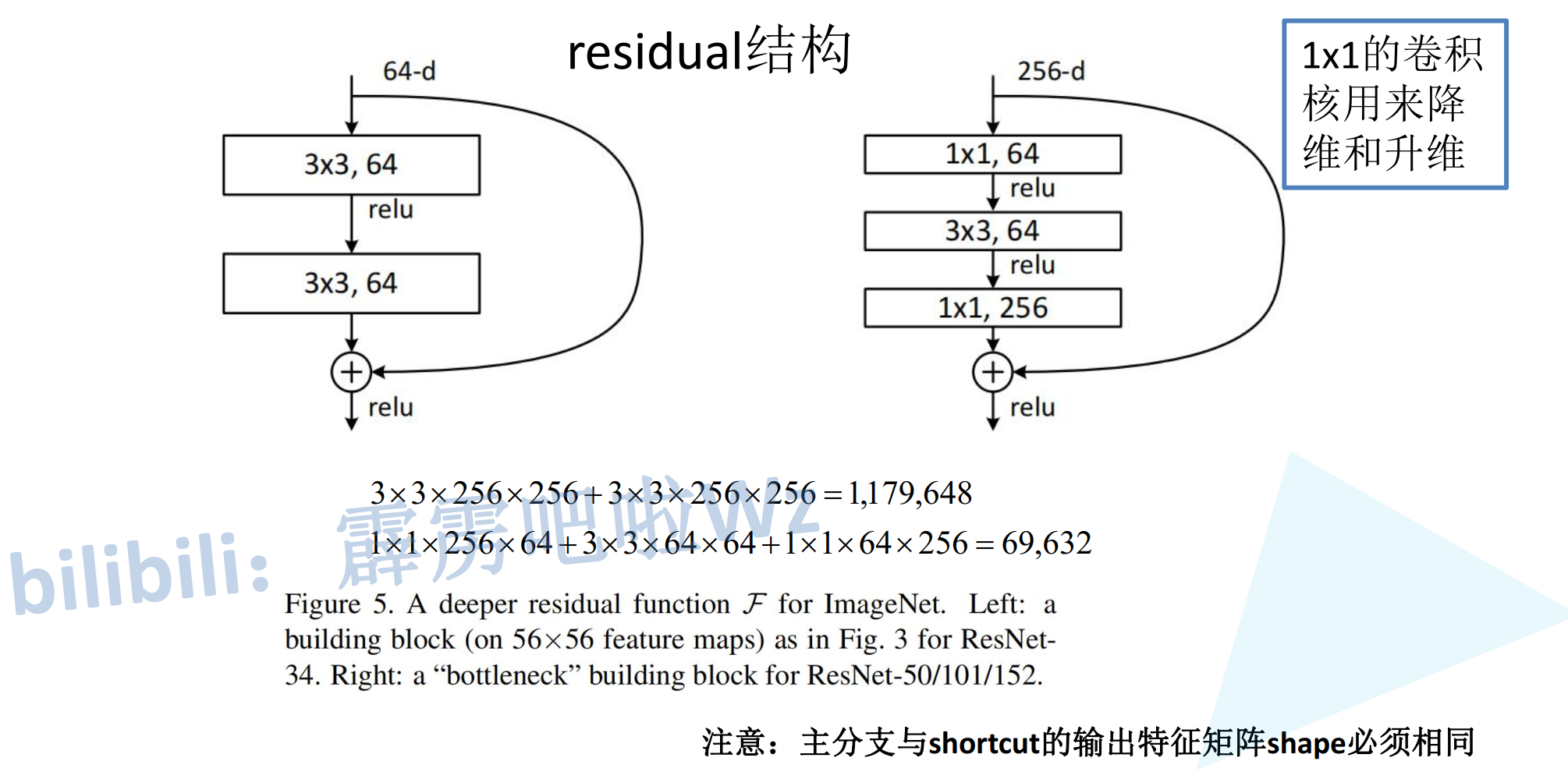
假设输入输出都是256通道：

两个3×3卷积(BasicBlock)：

参数量 = (256×3×3×256) × 2 = 1,179,648

1×1 + 3×3 + 1×1(Bottleneck，中间64通道)：

参数量 = 256×1×1×64 + 64×3×3×64 + 64×1×1×256 = 16,384 + 36,864 + 16,384 = 69,632

Bottleneck的参数量仅为BasicBlock的约1/17！

---

三、ResNet网络架构

3.1 整体结构

ResNet的整体网络架构如下：

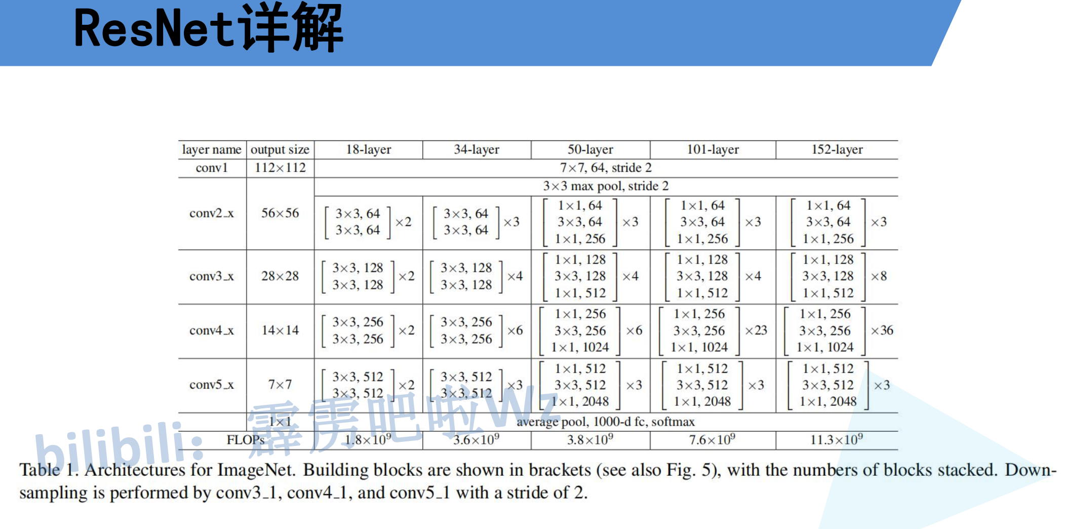
层名称	输出尺寸	ResNet-18	ResNet-34	ResNet-50	ResNet-101	ResNet-152
conv1	112×112	7×7, 64, stride 2	7×7, 64, stride 2	7×7, 64, stride 2	7×7, 64, stride 2	7×7, 64, stride 2
maxpool	56×56	3×3, stride 2	3×3, stride 2	3×3, stride 2	3×3, stride 2	3×3, stride 2
layer1	56×56	[3×3, 64] × 2	[3×3, 64] × 3	[1×1, 64; 3×3, 64; 1×1, 256] × 3	[1×1, 64; 3×3, 64; 1×1, 256] × 3	[1×1, 64; 3×3, 64; 1×1, 256] × 3
layer2	28×28	[3×3, 128] × 2	[3×3, 128] × 4	[1×1, 128; 3×3, 128; 1×1, 512] × 4	[1×1, 128; 3×3, 128; 1×1, 512] × 4	[1×1, 128; 3×3, 128; 1×1, 512] × 8
layer3	14×14	[3×3, 256] × 2	[3×3, 256] × 6	[1×1, 256; 3×3, 256; 1×1, 1024] × 6	[1×1, 256; 3×3, 256; 1×1, 1024] × 23	[1×1, 256; 3×3, 256; 1×1, 1024] × 36
layer4	7×7	[3×3, 512] × 2	[3×3, 512] × 3	[1×1, 512; 3×3, 512; 1×1, 2048] × 3	[1×1, 512; 3×3, 512; 1×1, 2048] × 3	[1×1, 512; 3×3, 512; 1×1, 2048] × 3
avgpool	1×1	全局平均池化	全局平均池化	全局平均池化	全局平均池化	全局平均池化
fc	num_classes	512 → num_classes	512 → num_classes	2048 → num_classes	2048 → num_classes	2048 → num_classes

3.3 虚线残差结构详解

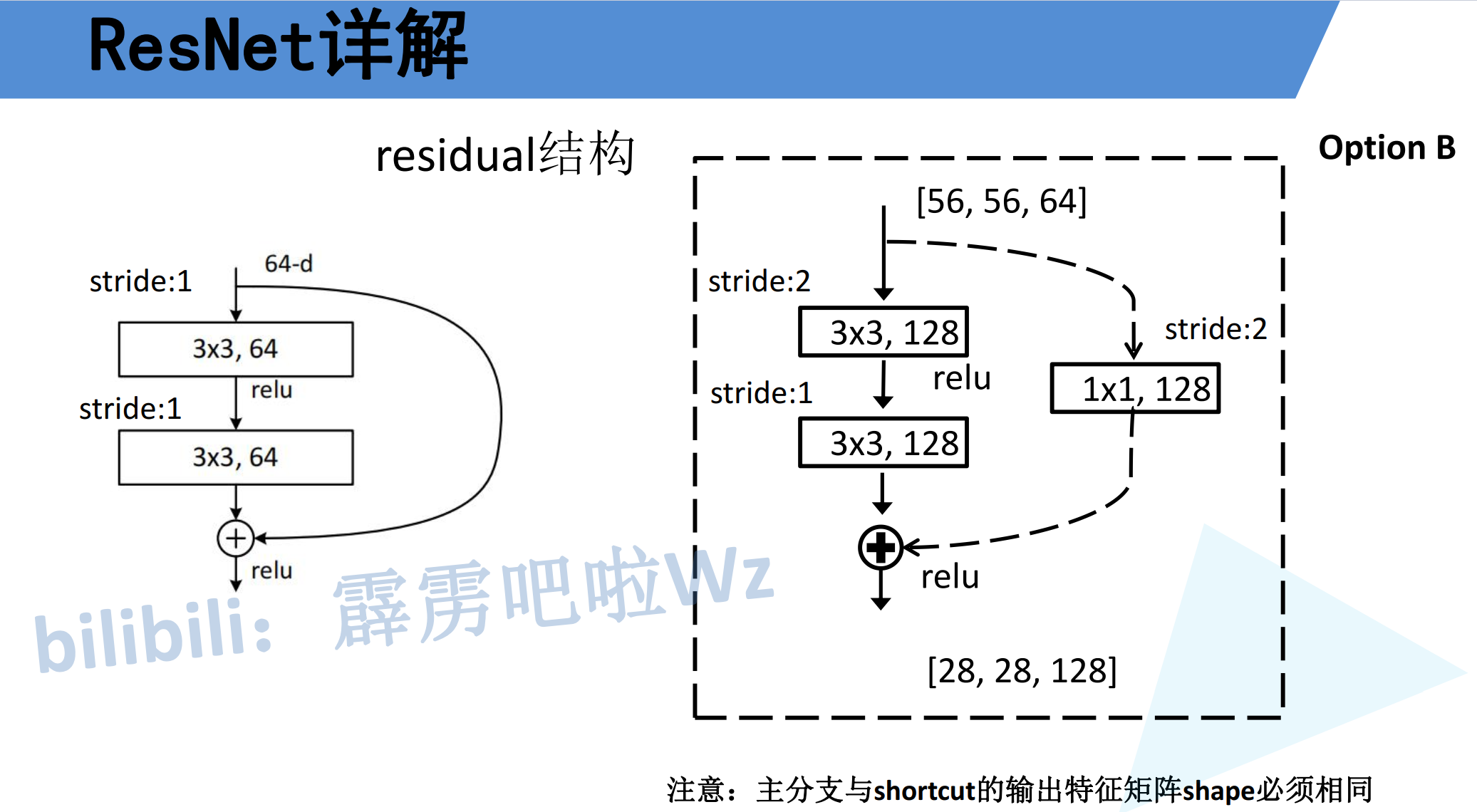
当输入输出维度不匹配时，需要通过downsample分支调整维度：

def _make_layer(self, block, channel, block_num, stride=1):
    downsample = None
    # 当stride不为1或输入输出通道不匹配时，需要downsample
    if stride != 1 or self.in_channel != channel * block.expansion:
        downsample = nn.Sequential(
            nn.Conv2d(self.in_channel, channel * block.expansion, 
                      kernel_size=1, stride=stride, bias=False),
            nn.BatchNorm2d(channel * block.expansion)
        )

    layers = []
    layers.append(block(self.in_channel, channel,
                        downsample=downsample,
                        stride=stride,
                        groups=self.groups,
                        width_per_group=self.width_per_group))
    self.in_channel = channel * block.expansion

    for _ in range(1, block_num):
        layers.append(block(self.in_channel, channel,
                            groups=self.groups,
                            width_per_group=self.width_per_group))

    return nn.Sequential(*layers)

3.4 BN层

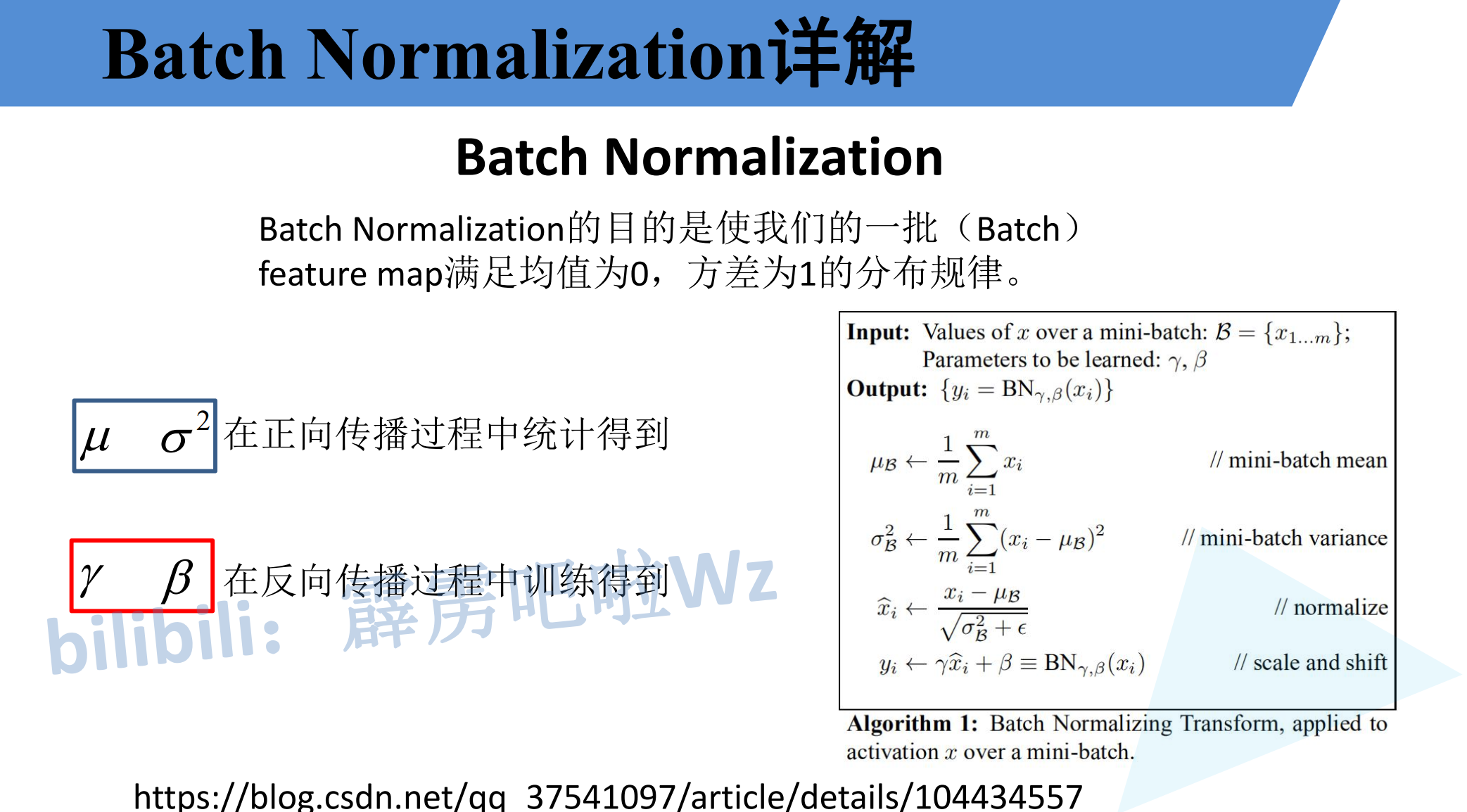
reset中引入了BN层：
Batch Normalization：每个卷积层后都接BN层，加速收敛。虽然数据预处理能够让输入满足均值为0，方差为1的分布规律。但经过卷积层之后就不一定满足了，因此reset提出了每个卷积层后都链接BN层，让其满足均值为0，方差为1的分布规律。

四、ResNet完整代码实现

4.1 完整网络代码

class ResNet(nn.Module):
    def __init__(self, block, blocks_num, num_classes=1000, include_top=True,
                 groups=1, width_per_group=64):
        super(ResNet, self).__init__()
        self.include_top = include_top
        self.in_channel = 64

        self.groups = groups
        self.width_per_group = width_per_group

        # 初始卷积层
        self.conv1 = nn.Conv2d(3, self.in_channel, kernel_size=7, stride=2,
                               padding=3, bias=False)
        self.bn1 = nn.BatchNorm2d(self.in_channel)
        self.relu = nn.ReLU(inplace=True)
        self.maxpool = nn.MaxPool2d(kernel_size=3, stride=2, padding=1)

        # 残差层
        self.layer1 = self._make_layer(block, 64, blocks_num[0])
        self.layer2 = self._make_layer(block, 128, blocks_num[1], stride=2)
        self.layer3 = self._make_layer(block, 256, blocks_num[2], stride=2)
        self.layer4 = self._make_layer(block, 512, blocks_num[3], stride=2)

        # 分类器
        if self.include_top:
            self.avgpool = nn.AdaptiveAvgPool2d((1, 1))
            self.fc = nn.Linear(512 * block.expansion, num_classes)

        # 权重初始化
        for m in self.modules():
            if isinstance(m, nn.Conv2d):
                nn.init.kaiming_normal_(m.weight, mode='fan_out', nonlinearity='relu')

    def forward(self, x):
        x = self.conv1(x)
        x = self.bn1(x)
        x = self.relu(x)
        x = self.maxpool(x)

        x = self.layer1(x)
        x = self.layer2(x)
        x = self.layer3(x)
        x = self.layer4(x)

        if self.include_top:
            x = self.avgpool(x)
            x = torch.flatten(x, 1)
            x = self.fc(x)

        return x

4.2 不同配置的ResNet

def resnet34(num_classes=1000, include_top=True):
    # ResNet-34: BasicBlock, [3, 4, 6, 3]
    return ResNet(BasicBlock, [3, 4, 6, 3], 
                  num_classes=num_classes, include_top=include_top)

def resnet50(num_classes=1000, include_top=True):
    # ResNet-50: Bottleneck, [3, 4, 6, 3]
    return ResNet(Bottleneck, [3, 4, 6, 3], 
                  num_classes=num_classes, include_top=include_top)

def resnet101(num_classes=1000, include_top=True):
    # ResNet-101: Bottleneck, [3, 4, 23, 3]
    return ResNet(Bottleneck, [3, 4, 23, 3], 
                  num_classes=num_classes, include_top=include_top)

def resnext50_32x4d(num_classes=1000, include_top=True):
    # ResNeXt-50: groups=32, width_per_group=4
    groups = 32
    width_per_group = 4
    return ResNet(Bottleneck, [3, 4, 6, 3],
                  num_classes=num_classes,
                  include_top=include_top,
                  groups=groups,
                  width_per_group=width_per_group)

---

五、训练过程

5.1 训练代码

def main():
    device = torch.device("cuda:0" if torch.cuda.is_available() else "cpu")

    # 数据预处理（使用ImageNet标准化）
    data_transform = {
        "train": transforms.Compose([
            transforms.RandomResizedCrop(224),
            transforms.RandomHorizontalFlip(),
            transforms.ToTensor(),
            transforms.Normalize([0.485, 0.456, 0.406], [0.229, 0.224, 0.225])
        ]),
        "val": transforms.Compose([
            transforms.Resize(256),
            transforms.CenterCrop(224),
            transforms.ToTensor(),
            transforms.Normalize([0.485, 0.456, 0.406], [0.229, 0.224, 0.225])
        ])
    }

    # 创建网络并加载预训练权重
    net = resnet34()
    model_weight_path = "./resnet34-pre.pth"
    net.load_state_dict(torch.load(model_weight_path, map_location='cpu'))

    # 修改全连接层以适应新的分类任务
    in_channel = net.fc.in_features
    net.fc = nn.Linear(in_channel, 5)  # 5类花卉分类
    net.to(device)

    # 损失函数和优化器
    loss_function = nn.CrossEntropyLoss()
    params = [p for p in net.parameters() if p.requires_grad]
    optimizer = optim.Adam(params, lr=0.0001)

    epochs = 3
    for epoch in range(epochs):
        net.train()
        for images, labels in train_loader:
            optimizer.zero_grad()
            logits = net(images.to(device))
            loss = loss_function(logits, labels.to(device))
            loss.backward()
            optimizer.step()

        # 验证
        net.eval()
        # ... 验证代码

5.2 训练技巧

1. Batch Normalization：模型内每个卷积层后都接BN层，加速收敛
2. 预训练权重：使用ImageNet预训练权重进行迁移学习
3. 学习率：使用较小的学习率（0.0001）进行微调
4. 数据增强：RandomResizedCrop、RandomHorizontalFlip
5. 标准化：使用ImageNet的均值和标准差进行归一化

---

六、迁移学习总结

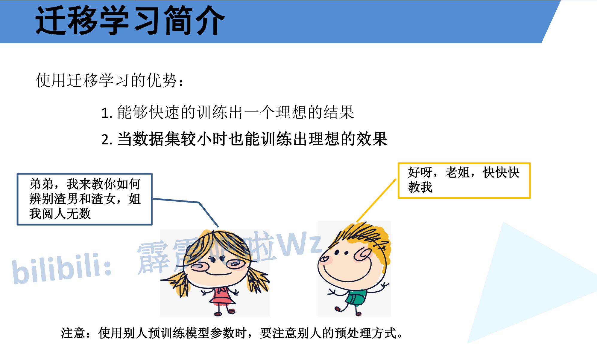
迁移学习的好处：
能够快速的训练出一个理想的结果

原因：我们不需要从随机初始化的参数开始训练。预训练模型已经具备了强大的、通用的特征提取能力。迁移学习相当于在一个非常高的起点上进行“微调”，让模型快速适应新任务的具体细节。

结果：极大地缩短了模型收敛所需的时间，能快速得到一个性能不错的模型。

当数据集较小时也能训练出理想的效果

原因：深度学习模型参数众多，从头训练需要海量数据来防止过拟合。如果我们的新任务数据集很小，直接训练复杂模型必然会失败。迁移学习利用了大模型在大数据上学到的、泛化能力强的特征作为基石，即使新数据很少，也能有效地进行微调。

结果：打破了“大数据依赖”，使得在小数据集上应用强大的深度学习模型成为可能，这是其最具实用价值的优势之一。

七、预测代码

import os
import json

import torch
from PIL import Image
from torchvision import transforms
import matplotlib.pyplot as plt

from model import resnet34


def main():
    device = torch.device("cuda:0" if torch.cuda.is_available() else "cpu")

    data_transform = transforms.Compose(
        [transforms.Resize(256),
         transforms.CenterCrop(224),
         transforms.ToTensor(),
         transforms.Normalize([0.485, 0.456, 0.406], [0.229, 0.224, 0.225])])

    # load image
    img_path = "../tulip.jpg"
    assert os.path.exists(img_path), "file: '{}' dose not exist.".format(img_path)
    img = Image.open(img_path)
    plt.imshow(img)
    # [N, C, H, W]
    img = data_transform(img)
    # expand batch dimension
    img = torch.unsqueeze(img, dim=0)

    # read class_indict
    json_path = './class_indices.json'
    assert os.path.exists(json_path), "file: '{}' dose not exist.".format(json_path)

    with open(json_path, "r") as f:
        class_indict = json.load(f)

    # create model
    model = resnet34(num_classes=5).to(device)

    # load model weights
    weights_path = "./resNet34.pth"
    assert os.path.exists(weights_path), "file: '{}' dose not exist.".format(weights_path)
    model.load_state_dict(torch.load(weights_path, map_location=device))

    # prediction
    model.eval()
    with torch.no_grad():
        # predict class
        output = torch.squeeze(model(img.to(device))).cpu()
        predict = torch.softmax(output, dim=0)
        predict_cla = torch.argmax(predict).numpy()

    print_res = "class: {}   prob: {:.3}".format(class_indict[str(predict_cla)],
                                                 predict[predict_cla].numpy())
    plt.title(print_res)
    for i in range(len(predict)):
        print("class: {:10}   prob: {:.3}".format(class_indict[str(i)],
                                                  predict[i].numpy()))
    plt.show()


if __name__ == '__main__':
    main()

没啥说的，都是以前模型提到的通用代码。

八、ResNet特点总结

8.1 优点

特点	说明
解决退化问题	残差学习使深层网络能够有效训练
缓解梯度消失	跳跃连接为梯度提供直接传播路径
易于优化	残差映射比直接映射更容易学习
参数高效	Bottleneck结构减少参数量
通用性强	可扩展到各种深度，广泛用于各种视觉任务

8.2 创新点

1. 残差学习框架：让网络学习残差映射而非直接映射
2. 跳跃连接：简单相加操作，不引入额外参数
3. Bottleneck结构：1×1卷积降维升维，大幅减少计算量
4. Batch Normalization：配合残差学习，加速深层网络训练

8.3 与其他网络对比

网络	年份	深度	Top-5错误率	核心创新
AlexNet	2012	8层	15.3%	ReLU、Dropout
VGG-16	2014	16层	7.3%	小卷积核堆叠
GoogLeNet	2014	22层	6.67%	Inception模块
ResNet-152	2015	152层	3.57%	残差学习

ResNet首次将网络深度提升到百层级别，并取得了超越人类的分类准确率，是深度学习发展史上的里程碑。

---

九、总结

ResNet通过引入残差学习框架和跳跃连接，成功解决了深度网络训练中的梯度消失和退化问题，使得训练超深层网络成为可能。其核心思想——让网络学习残差而非直接映射——简单而有效，对后续网络设计产生了深远影响。

ResNet的成功证明了：合理的网络结构设计比单纯增加深度更重要。残差连接已成为现代深度网络的标配组件，被广泛应用于各种架构中。

---