第七章 回归案例(三)客户流失预警逻辑回归
案例:客户流失预警
案例背景
本案例中所使用的数据集包括通信用户的流失与相关特征的数据,我们将使用逻辑回归,根据相关特征构建模型预测某用户的流失概率
数据读取读取与划分
在此案例中我们主要运用scipy库中的stats对数据做逻辑回归分析
import numpy as np
import pandas as pd
import seaborn as sns
import matplotlib.pyplot as plt

from scipy import stats
import statsmodels.api as sm
import statsmodels.formula.api as smf
首先,将我们的数据telecom_churn.csv读入,保存在变量churn中
然后我们对churn有个初步的认识
可以看到,有3463行数据,每组数据对应20个不同字段,且每个字段内包含的都是float64类型
churn = pd.read_csv('./telecom_churn.csv', skipinitialspace=True)
churn.head()
| subscriberID | churn | gender | AGE | edu_class | incomeCode | duration | feton | peakMinAv | peakMinDiff | posTrend | negTrend | nrProm | prom | curPlan | avgplan | planChange | posPlanChange | negPlanChange | call_10086 | |
|---|---|---|---|---|---|---|---|---|---|---|---|---|---|---|---|---|---|---|---|---|
| 0 | 19164958.0 | 1.0 | 0.0 | 20.0 | 2.0 | 12.0 | 16.0 | 0.0 | 113.666667 | -8.0 | 0.0 | 1.0 | 0.0 | 0.0 | 1.0 | 1.0 | 0.0 | 0.0 | 0.0 | 0.0 |
| 1 | 39244924.0 | 1.0 | 1.0 | 20.0 | 0.0 | 21.0 | 5.0 | 0.0 | 274.000000 | -371.0 | 0.0 | 1.0 | 2.0 | 1.0 | 3.0 | 2.0 | 2.0 | 1.0 | 0.0 | 1.0 |
| 2 | 39578413.0 | 1.0 | 0.0 | 11.0 | 1.0 | 47.0 | 3.0 | 0.0 | 392.000000 | -784.0 | 0.0 | 1.0 | 0.0 | 0.0 | 3.0 | 3.0 | 0.0 | 0.0 | 0.0 | 1.0 |
| 3 | 40992265.0 | 1.0 | 0.0 | 43.0 | 0.0 | 4.0 | 12.0 | 0.0 | 31.000000 | -76.0 | 0.0 | 1.0 | 2.0 | 1.0 | 3.0 | 3.0 | 0.0 | 0.0 | 0.0 | 1.0 |
| 4 | 43061957.0 | 1.0 | 1.0 | 60.0 | 0.0 | 9.0 | 14.0 | 0.0 | 129.333333 | -334.0 | 0.0 | 1.0 | 0.0 | 0.0 | 3.0 | 3.0 | 0.0 | 0.0 | 0.0 | 0.0 |
churn.info()
<class 'pandas.core.frame.DataFrame'>
RangeIndex: 3463 entries, 0 to 3462
Data columns (total 20 columns):
 #   Column         Non-Null Count  Dtype
---  ------         --------------  -----
 0   subscriberID   3463 non-null   float64
 1   churn          3463 non-null   float64
 2   gender         3463 non-null   float64
 3   AGE            3463 non-null   float64
 4   edu_class      3463 non-null   float64
 5   incomeCode     3463 non-null   float64
 6   duration       3463 non-null   float64
 7   feton          3463 non-null   float64
 8   peakMinAv      3463 non-null   float64
 9   peakMinDiff    3463 non-null   float64
 10  posTrend       3463 non-null   float64
 11  negTrend       3463 non-null   float64
 12  nrProm         3463 non-null   float64
 13  prom           3463 non-null   float64
 14  curPlan        3463 non-null   float64
 15  avgplan        3463 non-null   float64
 16  planChange     3463 non-null   float64
 17  posPlanChange  3463 non-null   float64
 18  negPlanChange  3463 non-null   float64
 19  call_10086     3463 non-null   float64
dtypes: float64(20)
memory usage: 541.2 KB
我们可以看到数据还是比较标准且基本无缺失值,为我们后续的研究提供了极大便利
首先,我们对数据进行简单的一元逻辑回归探索
猜想:posTrend 为 1,即流量使用有上升趋势时,更不容易流失(用得越多越不容易流失)
交叉表分析
cross_table = pd.crosstab(index=churn.posTrend, columns=churn.churn, margins=True)
cross_table
| churn | 0.0 | 1.0 | All |
|---|---|---|---|
| posTrend | |||
| 0.0 | 829 | 990 | 1819 |
| 1.0 | 1100 | 544 | 1644 |
| All | 1929 | 1534 | 3463 |
# 转化成百分比的形式:

def perConvert(ser):
    return ser/float(ser[-1])

cross_table.apply(perConvert, axis='columns')

# axis=1 也可以写成 axis='columns', 表示对列使用这个函数
# 发现的确如我们所想,流量使用有上升趋势的时候,流失的概率会下降
| churn | 0.0 | 1.0 | All |
|---|---|---|---|
| posTrend | |||
| 0.0 | 0.455745 | 0.544255 | 1.0 |
| 1.0 | 0.669100 | 0.330900 | 1.0 |
| All | 0.557031 | 0.442969 | 1.0 |
卡方检验
print("""chisq = %6.4f
p-value = %6.4f
dof = %i
expected_freq = %s""" % stats.chi2_contingency(observed=cross_table.iloc[:2, :2]))
# iloc 是因为 cross_table 添加了 margin 参数,也就是在最后一行和最后一列都显示 all,
 ## 卡方检验的时候我们只需要传入类别列即可,无需总列

# 发现检验结果还是比较显著的,说明 posTrend 这个变量有价值
chisq = 158.4433
p-value = 0.0000
dof = 1
expected_freq = [[1013.24025411  805.75974589]
 [ 915.75974589  728.24025411]]
一元逻辑回归模型搭建与训练
train = churn.sample(frac=0.7, random_state=1234).copy()
test = churn[~ churn.index.isin(train.index)].copy()
# ~ 表示取反,isin 表示在不在,这个知识点 pandas 非常常用
print(f'训练集样本量:{len(train)}, 测试集样本量:{len(test)}')
训练集样本量:2424, 测试集样本量:1039
statsmodels 库进行逻辑回归
# glm: general linear model - 也就是逻辑回归的别称:广义线性回归
lg = smf.glm(formula='churn ~ duration', data=churn,
            family=sm.families.Binomial(sm.families.links.logit())).fit()
            ## family=sm .... logit 这一大行看似难,其实只要是统计学库进行逻辑回归建模,
             ## 都是这样建,families 族群为 Binomial,即伯努利分布(0-1 分布)
lg.summary()
c:\environment\python38\lib\site-packages\statsmodels\genmod\families\links.py:13: FutureWarning: The logit link alias is deprecated. Use Logit instead. The logit link alias will be removed after the 0.15.0 release.
  warnings.warn(
| Dep. Variable: | churn | No. Observations: | 3463 |
|---|---|---|---|
| Model: | GLM | Df Residuals: | 3461 |
| Model Family: | Binomial | Df Model: | 1 |
| Link Function: | logit | Scale: | 1.0000 |
| Method: | IRLS | Log-Likelihood: | -1516.2 |
| Date: | Sat, 14 Oct 2023 | Deviance: | 3032.3 |
| Time: | 12:09:01 | Pearson chi2: | 2.78e+03 |
| No. Iterations: | 7 | Pseudo R-squ. (CS): | 0.3920 |
| Covariance Type: | nonrobust |
| coef | std err | z | P>|z| | [0.025 | 0.975] | |
|---|---|---|---|---|---|---|
| Intercept | 2.5883 | 0.100 | 25.767 | 0.000 | 2.391 | 2.785 |
| duration | -0.2482 | 0.009 | -26.424 | 0.000 | -0.267 | -0.230 |
从上面的结果可以看到逻辑回归的因变量是churn(是否流失),自变量duration(用户在网时长)的系数是-0.2482,说明用户在网时长每增加一个单位,客户流失的概率就平均下降24.82%,它的P值为0,说明它的结果在统计上显著可靠。
使用建模结果进行预测
# 预测流失的可能性
train['proba'] = lg.predict(train)
test['proba'] = lg.predict(test)
# 以 proba > 0.5 就设为流失作为预测结果
test['prediction'] = (test['proba'] > 0.5)*1

test[['churn', 'prediction']].sample(5)
| churn | prediction | |
|---|---|---|
| 722 | 1.0 | 0 |
| 2702 | 0.0 | 1 |
| 2397 | 0.0 | 0 |
| 3383 | 0.0 | 0 |
| 1786 | 0.0 | 1 |
检验预测结果
pd.crosstab(index=test.churn, columns=test.prediction, margins=True)
| prediction | 0 | 1 | All |
|---|---|---|---|
| churn | |||
| 0.0 | 427 | 156 | 583 |
| 1.0 | 88 | 368 | 456 |
| All | 515 | 524 | 1039 |
# 计算一下模型预测的准度如何
acc = sum(test['prediction'] == test['churn']) / len(test)
print(f'The accuracy is: {acc}')
The accuracy is: 0.7651588065447545
# sklearn 包绘制 Python 专门用来评估逻辑回归模型精度的 ROC 曲线
import sklearn.metrics as metrics
fpr_test, tpr_test, th_test = metrics.roc_curve(test.churn, test.proba)
fpr_train, tpr_train, th_train = metrics.roc_curve(train.churn, train.proba)

plt.figure(figsize=[3, 3])
plt.plot(fpr_test, tpr_test, 'b--')
plt.plot(fpr_train, tpr_train, 'r--')
plt.title('ROC curve'); plt.show()

# 还可以,其实越靠近左上角越好

print(f'AUC = {metrics.auc(fpr_test, tpr_test)}')
# 模型精度比较高
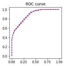
AUC = 0.8790154524389877
多元逻辑回归模型搭建与训练
逐步向前法筛选变量
逐步向前法是一种常用于特征选择的方法,特别适用于机器学习和统计建模中的回归分析。其基本思想是从一个空模型开始,逐步地向模型中加入一个个特征,每次加入一个特征后,评估模型的性能,并选择对性能改善最大的特征加入模型中,重复这个过程直到满足某个停止准则。
当然,这里的变量还不算特别特别多,还可以使用分层抽样,假设检验,方差分析等方法筛选
这里不用多解释了,逻辑回归的逐步向前法已有优秀前人的轮子,直接拿来用即可
逐步向前法筛选变量时,线性回归与逻辑回归的代码差别看下面这个代码框的注释即可
def forward_select(data, response):
    remaining = set(data.columns)
    remaining.remove(response)
    selected = []
    current_score, best_new_score = float('inf'), float('inf')
    while remaining:
        aic_with_candidates=[]
        for candidate in remaining:
            formula = "{} ~ {}".format(
                response,' + '.join(selected + [candidate]))
            aic = smf.glm(
                formula=formula, data=data,
                family=sm.families.Binomial(sm.families.links.logit())
                # 多元线性回归与多元逻辑回归的不同
            ).fit().aic
            aic_with_candidates.append((aic, candidate))
        aic_with_candidates.sort(reverse=True)
        best_new_score, best_candidate=aic_with_candidates.pop()
        if current_score > best_new_score:
            remaining.remove(best_candidate)
            selected.append(best_candidate)
            current_score = best_new_score
            print ('aic is {},continuing!'.format(current_score))
        else:
            print ('forward selection over!')
            break

    formula = "{} ~ {} ".format(response,' + '.join(selected))
    print('final formula is {}'.format(formula))
    model = smf.glm(
        formula=formula, data=data,
        family=sm.families.Binomial(sm.families.links.logit())
    ).fit()
    return(model)
# 待放入的变量,除了 subsriberID 没用外,其他都可以放进去看下
candidates = churn.columns.tolist()[1:]
data_for_select = train[candidates]
lg_m1 = forward_select(data=data_for_select, response='churn')
lg_m1.summary()
aic is 2139.9815513388403,continuing!
aic is 2015.248766843252,continuing!
aic is 1881.937082067902,continuing!
aic is 1824.2267798372745,continuing!
aic is 1768.3126157284164,continuing!
aic is 1720.3724820021637,continuing!
aic is 1698.6276836135844,continuing!
aic is 1694.3503537722104,continuing!
aic is 1685.9691682316302,continuing!
aic is 1683.5274343084689,continuing!
aic is 1677.5174259811881,continuing!
aic is 1675.025740842283,continuing!
| Dep. Variable: | churn | No. Observations: | 2424 |
|---|---|---|---|
| Model: | GLM | Df Residuals: | 2410 |
| Model Family: | Binomial | Df Model: | 13 |
| Link Function: | logit | Scale: | 1.0000 |
| Method: | IRLS | Log-Likelihood: | -823.14 |
| Date: | Sat, 14 Oct 2023 | Deviance: | 1646.3 |
| Time: | 12:09:03 | Pearson chi2: | 1.88e+03 |
| No. Iterations: | 7 | Pseudo R-squ. (CS): | 0.5009 |
| Covariance Type: | nonrobust |
| coef | std err | z | P>|z| | [0.025 | 0.975] | |
|---|---|---|---|---|---|---|
| Intercept | 4.7601 | 0.470 | 10.133 | 0.000 | 3.839 | 5.681 |
| duration | -0.2917 | 0.015 | -19.969 | 0.000 | -0.320 | -0.263 |
| feton | -1.4144 | 0.128 | -11.012 | 0.000 | -1.666 | -1.163 |
| gender | 1.4394 | 0.131 | 11.012 | 0.000 | 1.183 | 1.696 |
| call_10086 | -0.9040 | 0.126 | -7.161 | 0.000 | -1.151 | -0.657 |
| peakMinDiff | -0.0024 | 0.001 | -4.625 | 0.000 | -0.003 | -0.001 |
| edu_class | 0.5434 | 0.078 | 6.942 | 0.000 | 0.390 | 0.697 |
| AGE | -0.0195 | 0.005 | -4.255 | 0.000 | -0.029 | -0.011 |
| prom | 2.3925 | 0.693 | 3.451 | 0.001 | 1.034 | 3.751 |
| nrProm | -0.7430 | 0.248 | -2.993 | 0.003 | -1.230 | -0.256 |
| posTrend | -1.5598 | 0.416 | -3.747 | 0.000 | -2.376 | -0.744 |
| negTrend | -1.3003 | 0.414 | -3.138 | 0.002 | -2.113 | -0.488 |
| peakMinAv | 0.0011 | 0.000 | 2.289 | 0.022 | 0.000 | 0.002 |
| posPlanChange | -1.0211 | 0.624 | -1.637 | 0.102 | -2.244 | 0.202 |
方差膨胀因子检测
def vif(df, col_i):
    from statsmodels.formula.api import ols

    cols = list(df.columns)
    cols.remove(col_i)
    cols_noti = cols
    formula = col_i + '~' + '+'.join(cols_noti)
    r2 = ols(formula, df).fit().rsquared
    return 1. / (1. - r2)
after_select = lg_m1.params.index.tolist()[1:] # Intercept 不算
exog = train[after_select]
for i in exog.columns:
    print(i, '\t', vif(df=exog, col_i=i))
# 按照一般规则,大于10的就算全部超标,通常成对出现,只需要删除成对出现的一个即可。
 ## 这里我们挑成对出现中较大的删除
duration 	 1.161504699105813
feton 	 1.0328256567299994
gender 	 1.0133391644017549
call_10086 	 1.0312236075022612
peakMinDiff 	 1.751496545110971
edu_class 	 1.088991484453598
AGE 	 1.0509696212426345
prom 	 10.737528463052845
nrProm 	 10.65776904003062
posTrend 	 10.796864945899232
negTrend 	 10.721360755367611
peakMinAv 	 1.0986807256298052
posPlanChange 	 1.0556555380450348
# 删除 prom,posTrend
drop = ['prom', 'posTrend']
final_left = [x for x in after_select if x not in drop]

# 再来一次方差膨胀因子检测
exog = train[final_left]
for i in exog.columns:
    print(i, '\t', vif(df=exog, col_i=i))
# 方差膨胀因子合格了
duration 	 1.1589258261690667
feton 	 1.0319590476682936
gender 	 1.012938595864984
call_10086 	 1.0309266554767367
peakMinDiff 	 1.7195996869483132
edu_class 	 1.088768285735715
AGE 	 1.0479446481316026
nrProm 	 1.0040572241454906
negTrend 	 1.7000124717548541
peakMinAv 	 1.0469256802908604
posPlanChange 	 1.0120499617910743
再次进行建模与模型精度的检验
lg1 = smf.glm(formula='churn ~ duration + feton + gender + call_10086 + peakMinDiff + edu_class + AGE + nrProm + negTrend + peakMinAv + posPlanChange', data=churn,
            family=sm.families.Binomial(sm.families.links.logit())).fit()
# 预测流失的可能性
train['proba'] = lg1.predict(train)
test['proba'] = lg1.predict(test)
# 以 proba > 0.5 就设为流失作为预测结果
test['prediction'] = (test['proba'] > 0.5)*1
                        # 把 True 和 False 转化成 1 和 0
acc = sum(test['prediction'] == test['churn']) / len(test)
print(f'The accuracy is: {acc}')
The accuracy is: 0.8267564966313763
fpr_test, tpr_test, th_test = metrics.roc_curve(test.churn, test.proba)
fpr_train, tpr_train, th_train = metrics.roc_curve(train.churn, train.proba)

plt.figure(figsize=[3, 3])
plt.plot(fpr_test, tpr_test, 'b--')
plt.plot(fpr_train, tpr_train, 'r--')
plt.title('ROC curve')
plt.show()

# 还可以,其实越靠近左上角越好

print(f'AUC = {metrics.auc(fpr_test, tpr_test)}')
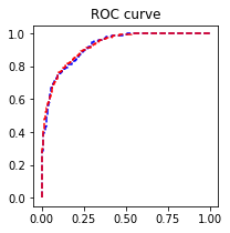
AUC = 0.9205861996328729

AtomGit 是由开放原子开源基金会联合 CSDN 等生态伙伴共同推出的新一代开源与人工智能协作平台。平台坚持“开放、中立、公益”的理念,把代码托管、模型共享、数据集托管、智能体开发体验和算力服务整合在一起,为开发者提供从开发、训练到部署的一站式体验。
更多推荐

 10
10 0
0- 0


 已为社区贡献6条内容

所有评论(0)