第七章 回归案例(一)波士顿房价预测
案例:波士顿房价预测
案例背景
在本小节中,我们将基于波士顿房价数据集建立线性回归模型,并对模型进行评估。该数据集可以使用sklearn自带的方法加载,我们将使用sklearn附带的一些工具来实现线性回归模型。sklearn.linear_model模块包含了常见的线性模型,即“预测目标能够表示成输入变量的线性组合形式”的模型。
数据读取与划分
首先我们导入将要使用的一些Python模块。
%matplotlib inline

import numpy as np
import pandas as pd
import scipy.stats as stats
import matplotlib.pyplot as plt
import statsmodels.api as sm
import sklearn
首先我们读入数据,并且打印数据的信息
bos = pd.read_csv("./input/data.csv")
bos.info()
<class 'pandas.core.frame.DataFrame'>
RangeIndex: 506 entries, 0 to 505
Data columns (total 14 columns):
 #   Column   Non-Null Count  Dtype
---  ------   --------------  -----
 0   CRIM     506 non-null    float64
 1   ZN       506 non-null    float64
 2   INDUS    506 non-null    float64
 3   CHAS     506 non-null    float64
 4   NOX      506 non-null    float64
 5   RM       506 non-null    float64
 6   AGE      506 non-null    float64
 7   DIS      506 non-null    float64
 8   RAD      506 non-null    float64
 9   TAX      506 non-null    float64
 10  PTRATIO  506 non-null    float64
 11  B        506 non-null    float64
 12  LSTAT    506 non-null    float64
 13  PRICE    506 non-null    float64
dtypes: float64(14)
memory usage: 55.5 KB
其中特征的解释如下(来自http://lib.stat.cmu.edu/datasets/boston)
| 特征 | 解释 |
|---|---|
| CRIM | per capita crime rate by town |
| ZN | proportion of residential land zoned for lots over 25,000 sq.ft. |
| INDUS | proportion of non-retail business acres per town |
| CHAS | Charles River dummy variable (= 1 if tract bounds river; 0 otherwise) |
| NOX | nitric oxides concentration (parts per 10 million) |
| RM | average number of rooms per dwelling |
| AGE | proportion of owner-occupied units built prior to 1940 |
| DIS | weighted distances to five Boston employment centres |
| RAD | index of accessibility to radial highways |
| TAX | full-value property-tax rate per $10,000 |
| PTRATIO | pupil-teacher ratio by town |
| B | 1000(Bk - 0.63)^2 where Bk is the proportion of blacks by town |
| LSTAT | % lower status of the population |
可见,数据集共包含506个样本。每个样本包含13个自变量和一个预测变量PRICE,接着打印数据的值
bos.head()
| CRIM | ZN | INDUS | CHAS | NOX | RM | AGE | DIS | RAD | TAX | PTRATIO | B | LSTAT | PRICE | |
|---|---|---|---|---|---|---|---|---|---|---|---|---|---|---|
| 0 | 0.00632 | 18.0 | 2.31 | 0.0 | 0.538 | 6.575 | 65.2 | 4.0900 | 1.0 | 296.0 | 15.3 | 396.90 | 4.98 | 24.0 |
| 1 | 0.02731 | 0.0 | 7.07 | 0.0 | 0.469 | 6.421 | 78.9 | 4.9671 | 2.0 | 242.0 | 17.8 | 396.90 | 9.14 | 21.6 |
| 2 | 0.02729 | 0.0 | 7.07 | 0.0 | 0.469 | 7.185 | 61.1 | 4.9671 | 2.0 | 242.0 | 17.8 | 392.83 | 4.03 | 34.7 |
| 3 | 0.03237 | 0.0 | 2.18 | 0.0 | 0.458 | 6.998 | 45.8 | 6.0622 | 3.0 | 222.0 | 18.7 | 394.63 | 2.94 | 33.4 |
| 4 | 0.06905 | 0.0 | 2.18 | 0.0 | 0.458 | 7.147 | 54.2 | 6.0622 | 3.0 | 222.0 | 18.7 | 396.90 | 5.33 | 36.2 |
线性回归模型搭建及训练
下面我们通过线性回归构建房价预测模型,回归系数使用最小二乘法来估计。
在我们的例子中 y = 波士顿房价。 X = 其余的输入变量。
首先,我们导入sklearn的linear_model模块。
然后将预测变量从DataFrame中删除。
最后创建一个线性模型对象lm。
from sklearn.linear_model import LinearRegression

X = bos.drop("PRICE", axis = 1)

lm = LinearRegression()
lm
LinearRegression()In a Jupyter environment, please rerun this cell to show the HTML representation or trust the notebook.
On GitHub, the HTML representation is unable to render, please try loading this page with nbviewer.org.
LinearRegression()
在进一步构建模型之前,我们简单介绍一下LinearRegression类。
它包含许多方法,其中以下三个方法是我们重点使用的方法。
lm.fit(): 训练一个线性模型lm.predict(): 利用训练好的线性模型进行预测lm.score():返回线性模型的决定系数R2R^2R2。
在完成模型训练后,我们可以通过lm.coef_和lm.intecept_获取回归系数和截距。
下面将使用13个自变量来预测房价。.fit()方法还有两个常用的参数可以设置:是否训练截距项和是否需要对数据进行标准化。
lm.fit(X, bos['PRICE'])
LinearRegression()In a Jupyter environment, please rerun this cell to show the HTML representation or trust the notebook.
On GitHub, the HTML representation is unable to render, please try loading this page with nbviewer.org.
LinearRegression()
查看回归系数和截距。
print("截距为:", lm.intercept_)
print ("回归系数为:", lm.coef_)
截距为: 36.45948838508977
回归系数为: [-1.08011358e-01  4.64204584e-02  2.05586264e-02  2.68673382e+00
 -1.77666112e+01  3.80986521e+00  6.92224640e-04 -1.47556685e+00
  3.06049479e-01 -1.23345939e-02 -9.52747232e-01  9.31168327e-03
 -5.24758378e-01]
为了便于分析,我们将特征、回归系数以及P值组合成一个DataFrame对象。
model = sm.OLS( bos['PRICE'], X).fit()
p_values = model.summary2().tables[1]['P>|t|']
pd.DataFrame(list(zip(X.columns, lm.coef_,p_values)), columns=["特征","回归系数","P值"])
| 特征 | 回归系数 | P值 | |
|---|---|---|---|
| 0 | CRIM | -0.108011 | 7.197130e-03 |
| 1 | ZN | 0.046420 | 7.762640e-04 |
| 2 | INDUS | 0.020559 | 9.497886e-01 |
| 3 | CHAS | 2.686734 | 1.689461e-03 |
| 4 | NOX | -17.766611 | 3.935067e-01 |
| 5 | RM | 3.809865 | 1.179476e-61 |
| 6 | AGE | 0.000692 | 5.989795e-01 |
| 7 | DIS | -1.475567 | 1.016889e-06 |
| 8 | RAD | 0.306049 | 1.064354e-02 |
| 9 | TAX | -0.012335 | 1.698772e-02 |
| 10 | PTRATIO | -0.952747 | 3.925055e-04 |
| 11 | B | 0.009312 | 5.266943e-08 |
| 12 | LSTAT | -0.524758 | 2.142519e-15 |
数据可视化与分析
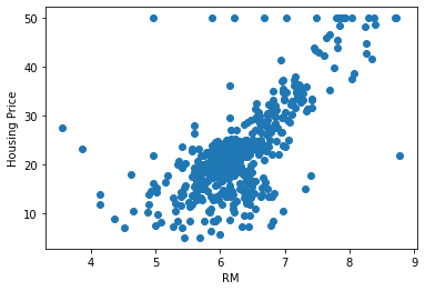
plt.scatter(bos.RM,bos.PRICE)
plt.xlabel("RM")
plt.ylabel("Housing Price")
plt.show()
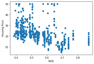
plt.scatter(bos.NOX,bos.PRICE)
plt.xlabel("NOX")
plt.ylabel("Housing Price")
plt.show()
首先我们通过训练好的线性模型得到模型在数据集上的预测值。
lm.predict(X)[0:5]
array([30.00384338, 25.02556238, 30.56759672, 28.60703649, 27.94352423])
绘制散点图,对比模型预测的房价与真实房价之间的关系。
plt.scatter(bos.PRICE,lm.predict(X))
plt.plot([0,50], [0,50], linewidth=1, color='red')
plt.xlabel("Prices: $y_i$")
plt.ylabel("Predicted prices: $\hat{y}_i$")
plt.show()
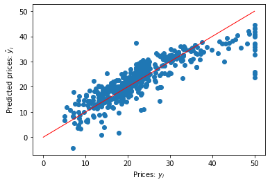
可见模型并不能100%准确预测房价,模型会有预测误差。特别是在高房价的房子中,模型的预测效果较差。
最常见的评估模型误差的指标为均方误差。
mseFull = np.mean((bos.PRICE - lm.predict(X))**2)
print("mseFull", mseFull)
mseFull 21.894831181729206
模型评估
上述均方误差是在训练集上计算的。实际项目中我们需要一份单独的测试数据用来测试模型效果。
在sklearn中我们可以使用model_selection模块的train_test_split方法进行训练集和测试集划分。
X_train, X_test, Y_train, Y_test = sklearn.model_selection.train_test_split(X, bos.PRICE,
    test_size=0.33, random_state=5)
使用训练集训练线性模型。
lm = LinearRegression()
lm.fit(X_train, Y_train)
pred_train = lm.predict(X_train)
pred_test = lm.predict(X_test)
print ("训练误差为:", np.mean((Y_train - pred_train) ** 2))
print ("测试误差为:", np.mean((Y_test - pred_test) ** 2))
训练误差为: 19.546758473534663
测试误差为: 28.530458765974643
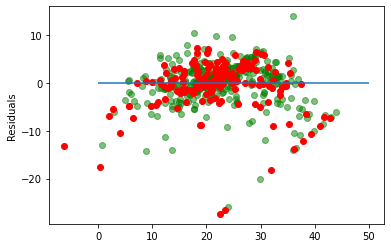
残差图是一种用来诊断回归模型效果的图。在残差图中,如果点随机分布在0附近,则说明回归效果较好。
如果在残差图中发现了某种结构,则说明回归效果不佳,需要重新建模。
plt.scatter(pred_train, pred_train - Y_train, c="g", alpha=0.5)
plt.scatter(pred_test, pred_test - Y_test, c="r")
plt.hlines(y=0, xmin=0, xmax=50)
plt.ylabel("Residuals")
Text(0, 0.5, 'Residuals')

AtomGit 是由开放原子开源基金会联合 CSDN 等生态伙伴共同推出的新一代开源与人工智能协作平台。平台坚持“开放、中立、公益”的理念,把代码托管、模型共享、数据集托管、智能体开发体验和算力服务整合在一起,为开发者提供从开发、训练到部署的一站式体验。
更多推荐

 10
10 0
0- 0


 已为社区贡献6条内容

所有评论(0)