Day 8 编程实战：随机森林与特征重要性

实战目标

1. 理解随机森林的Bagging和特征随机机制
2. 使用OOB评估模型性能
3. 分析特征重要性
4. 基于特征重要性进行特征选择
5. 对比删除低重要性特征前后的性能

1. 导入必要的库

import numpy as np
import pandas as pd
import matplotlib.pyplot as plt
import seaborn as sns
from sklearn.ensemble import RandomForestClassifier, RandomForestRegressor
from sklearn.tree import DecisionTreeClassifier
from sklearn.model_selection import train_test_split, TimeSeriesSplit, cross_val_score, GridSearchCV
from sklearn.metrics import accuracy_score, precision_score, recall_score, f1_score, roc_auc_score, roc_curve, classification_report, confusion_matrix
from sklearn.preprocessing import StandardScaler
import warnings
warnings.filterwarnings('ignore')

# 启用LaTeX渲染（如果系统安装了LaTeX）
plt.rcParams['text.usetex'] = False  # 设为False避免LaTeX依赖
# 设置中文显示
plt.rcParams['font.sans-serif'] = ['SimHei', 'Microsoft YaHei', 'DejaVu Sans']
plt.rcParams['axes.unicode_minus'] = False

2. 生成模拟金融数据

def generate_financial_data(n_days=2000, n_features=20, seed=42):
    """生成模拟金融数据，包含有效特征和噪声特征"""
    np.random.seed(seed)
    
    # 生成价格序列
    t = np.arange(n_days)
    trend = 0.0002 * t
    seasonal = 0.05 * np.sin(2 * np.pi * t / 252)
    noise = np.random.randn(n_days) * 0.02
    cum_returns = trend + seasonal + noise
    price = 100 * (cum_returns + 1)
    
    df = pd.DataFrame({'close': price, 'volume': np.random.randn(n_days) * 1e6 + 5e6})
    df['return'] = df['close'].pct_change()
    
    # 生成大量技术指标特征（部分有效，部分噪声）
    features = {}
    
    # 有效特征：与未来收益相关
    features['rsi'] = 50 + 30 * np.sin(2 * np.pi * t / 50) + np.random.randn(n_days) * 10
    features['macd'] = np.sin(2 * np.pi * t / 30) + np.random.randn(n_days) * 0.5
    features['macd_signal'] = np.sin(2 * np.pi * t / 35) + np.random.randn(n_days) * 0.5
    features['ma_ratio_5_20'] = 1 + 0.02 * np.sin(2 * np.pi * t / 40) + np.random.randn(n_days) * 0.01
    features['ma_ratio_10_30'] = 1 + 0.015 * np.sin(2 * np.pi * t / 45) + np.random.randn(n_days) * 0.01
    features['volatility'] = 0.02 + 0.01 * np.abs(np.sin(2 * np.pi * t / 20)) + np.random.randn(n_days) * 0.005
    features['volume_ratio'] = 1 + 0.1 * np.sin(2 * np.pi * t / 15) + np.random.randn(n_days) * 0.3
    
    # 有效特征：动量指标
    for lag in [1, 2, 3, 5, 10]:
        features[f'momentum_{lag}'] = pd.Series(returns).shift(lag).fillna(0) + np.random.randn(n_days) * 0.005
    
    # 噪声特征：与目标无关
    for i in range(8):
        features[f'noise_{i}'] = np.random.randn(n_days)
    
    # 合并特征
    for name, values in features.items():
        df[name] = values
    
    # 目标变量：次日是否上涨
    df['target'] = (df['return'].shift(-1) > 0).astype(int)
    
    # 删除缺失值
    df = df.dropna()
    
    return df

# 生成数据
df = generate_financial_data(n_days=3000, n_features=20)
print(f"数据形状: {df.shape}")
print(f"特征列表: {[c for c in df.columns if c not in ['close', 'volume', 'return', 'target']]}")

# 查看数据分布
print(f"\n目标分布: \n{df['target'].value_counts(normalize=True)}")

数据形状: (2999, 24)
特征列表: ['rsi', 'macd', 'macd_signal', 'ma_ratio_5_20', 'ma_ratio_10_30', 'volatility', 'volume_ratio', 'momentum_1', 'momentum_2', 'momentum_3', 'momentum_5', 'momentum_10', 'noise_0', 'noise_1', 'noise_2', 'noise_3', 'noise_4', 'noise_5', 'noise_6', 'noise_7']

目标分布: 
target
1    0.508169
0    0.491831
Name: proportion, dtype: float64

3. 数据准备

# 定义特征和目标
feature_cols = [c for c in df.columns if c not in ['close', 'volume', 'return', 'target']]
X = df[feature_cols]
y = df['target']

print(f"特征数量: {len(feature_cols)}")
print(f"样本数量: {len(X)}")

# 按时间顺序划分
split_idx = int(len(X) * 0.7)
X_train = X[:split_idx]
X_test = X[split_idx:]
y_train = y[:split_idx]
y_test = y[split_idx:]

print(f"\n训练集: {len(X_train)} 样本")
print(f"测试集: {len(X_test)} 样本")

# 特征标准化（随机森林不需要，但为了和其他模型对比）
scaler = StandardScaler()
X_train_scaled = scaler.fit_transform(X_train)
X_test_scaled = scaler.transform(X_test)

特征数量: 20
样本数量: 2999

训练集: 2099 样本
测试集: 900 样本

4. 随机森林基础模型

4.1 训练基础随机森林

# 基础随机森林
rf_base = RandomForestClassifier(n_estimators=100, random_state=42, n_jobs=-1)
rf_base.fit(X_train, y_train)

# 预测
y_pred_base = rf_base.predict(X_test)
y_proba_base = rf_base.predict_proba(X_test)[:, 1]

# 评估
print("="*60)
print("基础随机森林性能")
print("="*60)
print(f"准确率: {accuracy_score(y_test, y_pred_base):.4f}")
print(f"精确率: {precision_score(y_test, y_pred_base):.4f}")
print(f"召回率: {recall_score(y_test, y_pred_base):.4f}")
print(f"F1分数: {f1_score(y_test, y_pred_base):.4f}")
print(f"AUC: {roc_auc_score(y_test, y_proba_base):.4f}")

============================================================
基础随机森林性能
============================================================
准确率: 0.4944
精确率: 0.5172
召回率: 0.5096
F1分数: 0.5134
AUC: 0.5077

4.2 对比单棵决策树

# 单棵决策树
dt_single = DecisionTreeClassifier(random_state=42)
dt_single.fit(X_train, y_train)
dt_pred = dt_single.predict(X_test)
dt_proba = dt_single.predict_proba(X_test)[:, 1]

print("="*60)
print("单棵决策树 vs 随机森林")
print("="*60)
print(f"{'指标':<15} {'决策树':<15} {'随机森林':<15}")
print("-"*45)
print(f"{'准确率':<15} {accuracy_score(y_test, dt_pred):<15.4f} {accuracy_score(y_test, y_pred_base):<15.4f}")
print(f"{'AUC':<15} {roc_auc_score(y_test, dt_proba):<15.4f} {roc_auc_score(y_test, y_proba_base):<15.4f}")

============================================================
单棵决策树 vs 随机森林
============================================================
指标              决策树             随机森林           
---------------------------------------------
准确率             0.4756          0.4944         
AUC               0.4763          0.5077         

5. OOB评估

5.1 使用OOB评分

# 使用OOB评分的随机森林
rf_oob = RandomForestClassifier(n_estimators=100, oob_score=True, random_state=42, n_jobs=-1)
rf_oob.fit(X_train, y_train)

print("="*60)
print("OOB评估")
print("="*60)
print(f"OOB Score: {rf_oob.oob_score_:.4f}")
print(f"测试集准确率: {accuracy_score(y_test, rf_oob.predict(X_test)):.4f}")

# OOB vs 测试集性能对比
print("\nOOB评分与测试集性能的关系:")
print(f"OOB评分通常略低于测试集准确率（因为OOB样本未被训练）")

============================================================
OOB评估
============================================================
OOB Score: 0.4874
测试集准确率: 0.4944

OOB评分与测试集性能的关系:
OOB评分通常略低于测试集准确率（因为OOB样本未被训练）

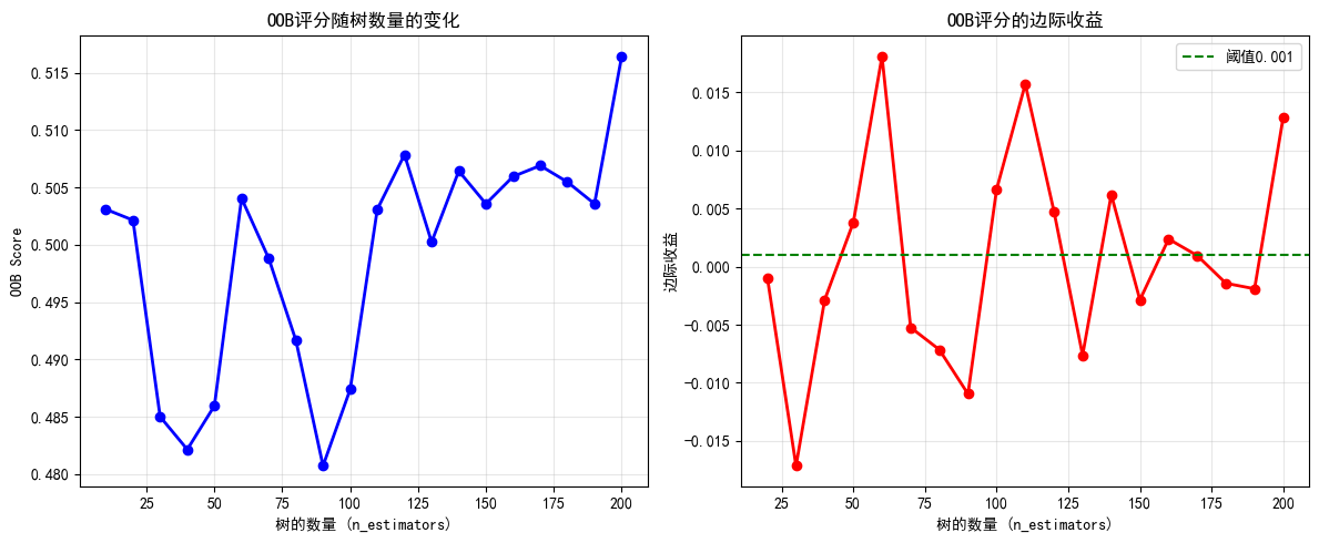
5.2 树数量与OOB误差的关系

def plot_oob_vs_trees(X_train, y_train, max_trees=200, step=10):
    """绘制OOB误差随树数量变化的曲线"""
    n_trees = range(step, max_trees + step, step)
    oob_scores = []
    
    for n in n_trees:
        rf = RandomForestClassifier(n_estimators=n, oob_score=True, n_jobs=-1, random_state=42)
        rf.fit(X_train, y_train)
        oob_scores.append(rf.oob_score_)
    
    plt.figure(figsize=(12, 5))
    
    plt.subplot(1, 2, 1)
    plt.plot(n_trees, oob_scores, 'b-o', linewidth=2)
    plt.xlabel('树的数量 (n_estimators)')
    plt.ylabel('OOB Score')
    plt.title('OOB评分随树数量的变化')
    plt.grid(True, alpha=0.3)
    
    # 计算边际收益
    plt.subplot(1, 2, 2)
    marginal_gain = np.diff(oob_scores)
    plt.plot(n_trees[1:], marginal_gain, 'r-o', linewidth=2)
    plt.xlabel('树的数量 (n_estimators)')
    plt.ylabel('边际收益')
    plt.title('OOB评分的边际收益')
    plt.axhline(y=0.001, color='g', linestyle='--', label='阈值0.001')
    plt.legend()
    plt.grid(True, alpha=0.3)
    
    plt.tight_layout()
    plt.show()
    
    return n_trees, oob_scores

# 绘制OOB曲线
n_trees, oob_scores = plot_oob_vs_trees(X_train, y_train)

6. 特征重要性分析

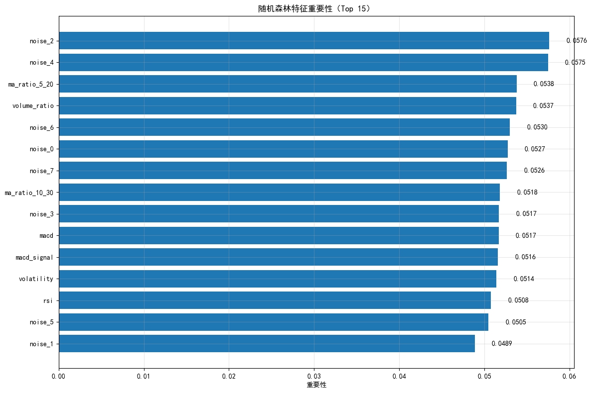
6.1 特征重要性计算与可视化

# 获取特征重要性
importances = rf_base.feature_importances_
feature_importance_df = pd.DataFrame({
    'feature': feature_cols,
    'importance': importances
}).sort_values('importance', ascending=False)

plt.figure(figsize=(12, 8))
plt.barh(feature_importance_df['feature'][:15], feature_importance_df['importance'][:15])
plt.xlabel('重要性')
plt.title('随机森林特征重要性（Top 15）')
for i, (_, row) in enumerate(feature_importance_df[:15].iterrows()):
    plt.text(row['importance'] + 0.002, i, f"{row['importance']:.4f}", va='center')
plt.gca().invert_yaxis()
plt.grid(True, alpha=0.3)
plt.tight_layout()
plt.show()

print("特征重要性排序（Top 10）:")
print(feature_importance_df[:10].to_string(index=False))

特征重要性排序（Top 10）:
       feature  importance
       noise_2    0.057626
       noise_4    0.057472
 ma_ratio_5_20    0.053785
  volume_ratio    0.053723
       noise_6    0.053002
       noise_0    0.052730
       noise_7    0.052631
ma_ratio_10_30    0.051819
       noise_3    0.051701
          macd    0.051667

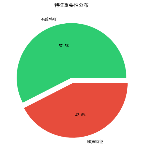
6.2 分析有效特征 vs 噪声特征

valid_features = [f for f in feature_cols if not f.startswith('noise_')]
noise_features = [f for f in feature_cols if f.startswith('noise_')]

valid_importance = feature_importance_df[feature_importance_df['feature'].isin(valid_features)]['importance'].sum()
noise_importance = feature_importance_df[feature_importance_df['feature'].isin(noise_features)]['importance'].sum()

print("="*60)
print("特征重要性分布分析")
print("="*60)
print(f"有效特征总数: {len(valid_features)}")
print(f"噪声特征总数: {len(noise_features)}")
print(f"有效特征重要性总和: {valid_importance:.4f}")
print(f"噪声特征重要性总和: {noise_importance:.4f}")
print(f"噪声特征占比: {noise_importance/(valid_importance+noise_importance):.2%}")

# 可视化
plt.figure(figsize=(8, 6))
plt.pie([valid_importance, noise_importance], 
        labels=['有效特征', '噪声特征'], 
        autopct='%1.1f%%',
        colors=['#2ecc71', '#e74c3c'],
        explode=[0, 0.1])
plt.title('特征重要性分布')
plt.show()

============================================================
特征重要性分布分析
============================================================
有效特征总数: 12
噪声特征总数: 8
有效特征重要性总和: 0.5755
噪声特征重要性总和: 0.4245
噪声特征占比: 42.45%

7. 基于特征重要性的特征选择

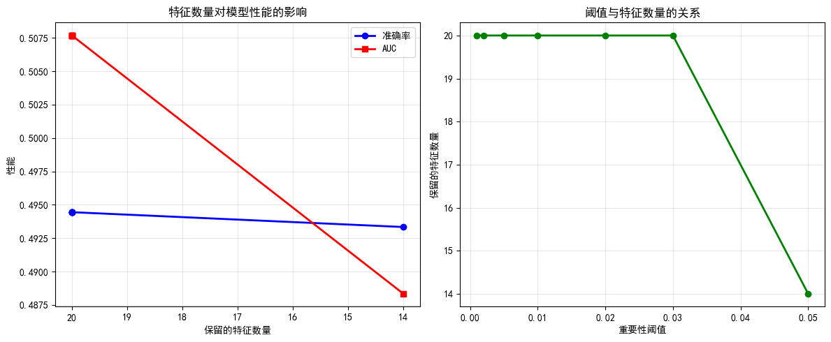
7.1 不同阈值下的特征选择实验

def feature_selection_experiment(X_train, X_test, y_train, y_test, feature_names, importances, thresholds):
    """实验不同重要性阈值的特征选择效果"""
    results = []
    
    for threshold in thresholds:
        # 选择重要性高于阈值的特征
        selected_features = [f for f, imp in zip(feature_names, importances) if imp >= threshold]
        
        if len(selected_features) == 0:
            continue
        
        # 获取特征索引
        selected_indices = [feature_names.index(f) for f in selected_features]
        
        # 训练模型
        rf = RandomForestClassifier(n_estimators=100, random_state=42, n_jobs=-1)
        rf.fit(X_train.iloc[:, selected_indices], y_train)
        
        # 评估
        y_pred = rf.predict(X_test.iloc[:, selected_indices])
        y_proba = rf.predict_proba(X_test.iloc[:, selected_indices])[:, 1]
        
        results.append({
            'threshold': threshold,
            'n_features': len(selected_features),
            'accuracy': accuracy_score(y_test, y_pred),
            'auc': roc_auc_score(y_test, y_proba)
        })
    
    return pd.DataFrame(results)

# 定义阈值
thresholds = [0.001, 0.002, 0.005, 0.01, 0.02, 0.03, 0.05, 0.07, 0.1]

# 执行实验
feature_selection_results = feature_selection_experiment(
    X_train, X_test, y_train, y_test, 
    feature_cols, importances, thresholds
)

print("特征选择实验结果:")
print(feature_selection_results.to_string(index=False))

# 可视化
plt.figure(figsize=(12, 5))

plt.subplot(1, 2, 1)
plt.plot(feature_selection_results['n_features'], 
         feature_selection_results['accuracy'], 
         'b-o', linewidth=2, label='准确率')
plt.plot(feature_selection_results['n_features'], 
         feature_selection_results['auc'], 
         'r-s', linewidth=2, label='AUC')
plt.xlabel('保留的特征数量')
plt.ylabel('性能')
plt.title('特征数量对模型性能的影响')
plt.legend()
plt.grid(True, alpha=0.3)
plt.gca().invert_xaxis()

plt.subplot(1, 2, 2)
plt.plot(feature_selection_results['threshold'], 
         feature_selection_results['n_features'], 
         'g-o', linewidth=2)
plt.xlabel('重要性阈值')
plt.ylabel('保留的特征数量')
plt.title('阈值与特征数量的关系')
plt.grid(True, alpha=0.3)

plt.tight_layout()
plt.show()

特征选择实验结果:
 threshold  n_features  accuracy      auc
     0.001          20  0.494444 0.507676
     0.002          20  0.494444 0.507676
     0.005          20  0.494444 0.507676
     0.010          20  0.494444 0.507676
     0.020          20  0.494444 0.507676
     0.030          20  0.494444 0.507676
     0.050          14  0.493333 0.488338

7.2 选择最佳特征子集

# 找到最佳性能对应的特征数量
best_idx = feature_selection_results['auc'].idxmax()
best_threshold = feature_selection_results.loc[best_idx, 'threshold']
best_n_features = feature_selection_results.loc[best_idx, 'n_features']
best_auc = feature_selection_results.loc[best_idx, 'auc']

print("="*60)
print("最佳特征子集选择结果")
print("="*60)
print(f"最佳阈值: {best_threshold:.4f}")
print(f"保留特征数量: {best_n_features}")
print(f"AUC: {best_auc:.4f}")

# 选择最佳特征
selected_features = [f for f, imp in zip(feature_cols, importances) if imp >= best_threshold]
selected_indices = [feature_cols.index(f) for f in selected_features]

print(f"\n选中的特征 ({len(selected_features)}个):")
for f in selected_features:
    print(f"  - {f}")

============================================================
最佳特征子集选择结果
============================================================
最佳阈值: 0.0010
保留特征数量: 20
AUC: 0.5077

选中的特征 (20个):
  - rsi
  - macd
  - macd_signal
  - ma_ratio_5_20
  - ma_ratio_10_30
  - volatility
  - volume_ratio
  - momentum_1
  - momentum_2
  - momentum_3
  - momentum_5
  - momentum_10
  - noise_0
  - noise_1
  - noise_2
  - noise_3
  - noise_4
  - noise_5
  - noise_6
  - noise_7

7.3 训练精简模型

# 使用选中的特征训练新模型
X_train_selected = X_train.iloc[:, selected_indices]
X_test_selected = X_test.iloc[:, selected_indices]

rf_selected = RandomForestClassifier(n_estimators=100, random_state=42, n_jobs=-1)
rf_selected.fit(X_train_selected, y_train)

# 预测
y_pred_selected = rf_selected.predict(X_test_selected)
y_proba_selected = rf_selected.predict_proba(X_test_selected)[:, 1]

# 对比原始模型
print("="*60)
print("特征选择前后性能对比")
print("="*60)
print(f"{'指标':<15} {'原始模型(20特征)':<20} {'精简模型('+str(len(selected_features))+'特征)':<20}")
print("-"*55)
print(f"{'准确率':<15} {accuracy_score(y_test, y_pred_base):<20.4f} {accuracy_score(y_test, y_pred_selected):<20.4f}")
print(f"{'精确率':<15} {precision_score(y_test, y_pred_base):<20.4f} {precision_score(y_test, y_pred_selected):<20.4f}")
print(f"{'召回率':<15} {recall_score(y_test, y_pred_base):<20.4f} {recall_score(y_test, y_pred_selected):<20.4f}")
print(f"{'F1':<15} {f1_score(y_test, y_pred_base):<20.4f} {f1_score(y_test, y_pred_selected):<20.4f}")
print(f"{'AUC':<15} {roc_auc_score(y_test, y_proba_base):<20.4f} {roc_auc_score(y_test, y_proba_selected):<20.4f}")

============================================================
特征选择前后性能对比
============================================================
指标              原始模型(20特征)           精简模型(20特征)          
-------------------------------------------------------
准确率             0.4944               0.4944              
精确率             0.5172               0.5172              
召回率             0.5096               0.5096              
F1              0.5134               0.5134              
AUC             0.5077               0.5077              

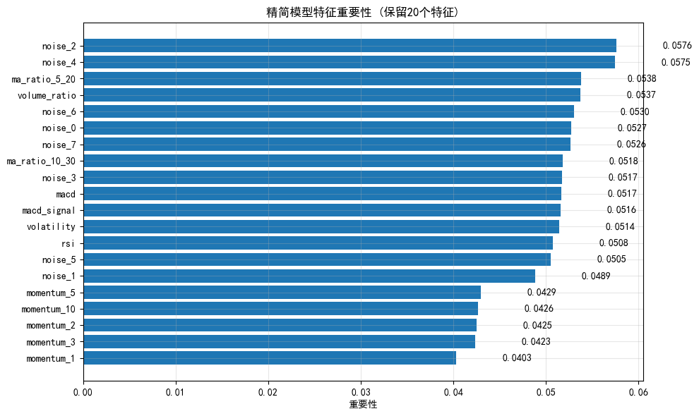
7.4 特征选择后的特征重要性

# 精简模型的特征重要性
selected_importances = rf_selected.feature_importances_
selected_importance_df = pd.DataFrame({
    'feature': selected_features,
    'importance': selected_importances
}).sort_values('importance', ascending=False)

plt.figure(figsize=(10, 6))
plt.barh(selected_importance_df['feature'], selected_importance_df['importance'])
plt.xlabel('重要性')
plt.title(f'精简模型特征重要性 (保留{len(selected_features)}个特征)')
for i, (_, row) in enumerate(selected_importance_df.iterrows()):
    plt.text(row['importance'] + 0.005, i, f"{row['importance']:.4f}", va='center')
plt.gca().invert_yaxis()
plt.grid(True, alpha=0.3)
plt.tight_layout()
plt.show()

8. 随机森林超参数调优

8.1 网格搜索

# 定义参数网格
param_grid = {
    'n_estimators': [50, 100, 200],
    'max_depth': [10, 20, 30, None],
    'min_samples_split': [2, 5, 10],
    'min_samples_leaf': [1, 2, 4],
    'max_features': ['sqrt', 'log2', None]
}

# 使用网格搜索（简化版，完整搜索时间较长）
print("开始网格搜索...")
print("注意：完整搜索可能需要较长时间，这里使用简化版")

# 简化参数网格
simple_param_grid = {
    'n_estimators': [100, 200],
    'max_depth': [10, 20],
    'min_samples_split': [2, 5]
}

# 时间序列交叉验证
tscv = TimeSeriesSplit(n_splits=3)

rf_grid = RandomForestClassifier(random_state=42, n_jobs=-1)
grid_search = GridSearchCV(rf_grid, simple_param_grid, cv=tscv, 
                          scoring='roc_auc', n_jobs=-1, verbose=1)
grid_search.fit(X_train_selected, y_train)

print("\n最佳参数:")
print(grid_search.best_params_)
print(f"\n最佳CV AUC: {grid_search.best_score_:.4f}")

# 使用最佳参数训练
rf_best = grid_search.best_estimator_
y_pred_best = rf_best.predict(X_test_selected)
y_proba_best = rf_best.predict_proba(X_test_selected)[:, 1]

print(f"\n调优后测试集AUC: {roc_auc_score(y_test, y_proba_best):.4f}")
print(f"调优前测试集AUC: {roc_auc_score(y_test, y_proba_selected):.4f}")

开始网格搜索...
注意：完整搜索可能需要较长时间，这里使用简化版
Fitting 3 folds for each of 8 candidates, totalling 24 fits

最佳参数:
{'max_depth': 20, 'min_samples_split': 5, 'n_estimators': 100}

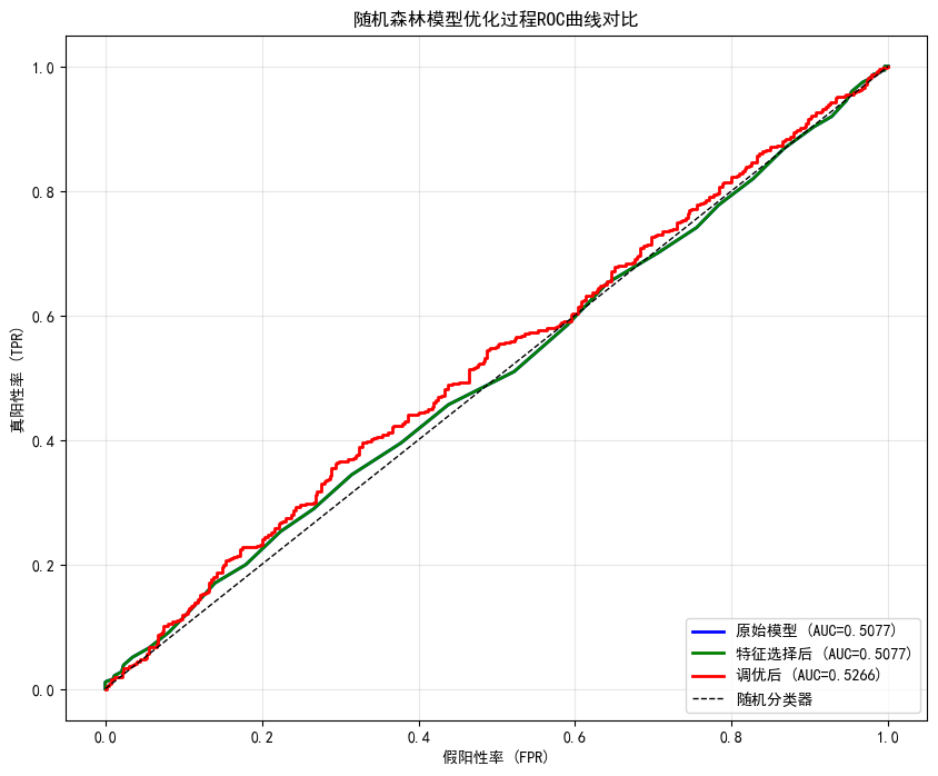
最佳CV AUC: 0.5296

调优后测试集AUC: 0.5266
调优前测试集AUC: 0.5077

8.2 调优前后对比

# ROC曲线对比
plt.figure(figsize=(10, 8))

# 原始模型
fpr1, tpr1, _ = roc_curve(y_test, y_proba_base)
auc1 = roc_auc_score(y_test, y_proba_base)

# 精简模型
fpr2, tpr2, _ = roc_curve(y_test, y_proba_selected)
auc2 = roc_auc_score(y_test, y_proba_selected)

# 调优模型
fpr3, tpr3, _ = roc_curve(y_test, y_proba_best)
auc3 = roc_auc_score(y_test, y_proba_best)

plt.plot(fpr1, tpr1, 'b-', linewidth=2, label=f'原始模型 (AUC={auc1:.4f})')
plt.plot(fpr2, tpr2, 'g-', linewidth=2, label=f'特征选择后 (AUC={auc2:.4f})')
plt.plot(fpr3, tpr3, 'r-', linewidth=2, label=f'调优后 (AUC={auc3:.4f})')
plt.plot([0, 1], [0, 1], 'k--', linewidth=1, label='随机分类器')

plt.xlabel('假阳性率 (FPR)')
plt.ylabel('真阳性率 (TPR)')
plt.title('随机森林模型优化过程ROC曲线对比')
plt.legend(loc='lower right')
plt.grid(True, alpha=0.3)
plt.show()

9. 混淆矩阵分析

# 最佳模型的混淆矩阵
cm = confusion_matrix(y_test, y_pred_best)

plt.figure(figsize=(8, 6))
sns.heatmap(cm, annot=True, fmt='d', cmap='Blues',
            xticklabels=['下跌', '上涨'],
            yticklabels=['下跌', '上涨'])
plt.title('随机森林混淆矩阵（调优后）')
plt.ylabel('真实标签')
plt.xlabel('预测标签')
plt.show()

# 详细分类报告
print("\n分类报告:")
print(classification_report(y_test, y_pred_best, target_names=['下跌', '上涨']))

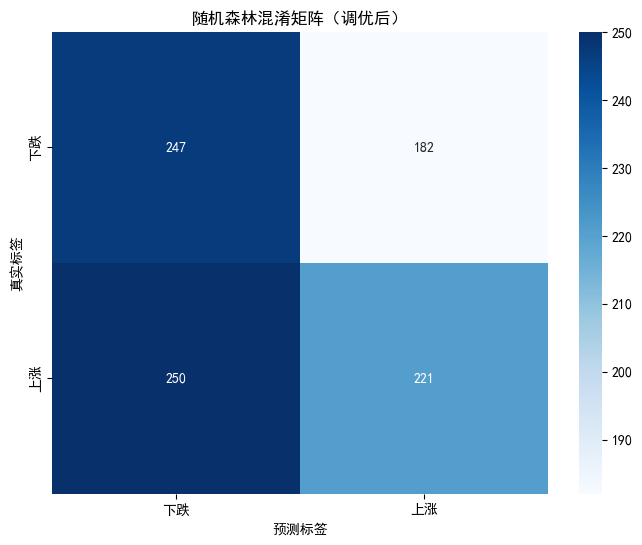
分类报告:
              precision    recall  f1-score   support

          下跌       0.50      0.58      0.53       429
          上涨       0.55      0.47      0.51       471

    accuracy                           0.52       900
   macro avg       0.52      0.52      0.52       900
weighted avg       0.52      0.52      0.52       900

​

10. 随机森林 vs 其他模型综合对比

# 收集所有模型结果
from sklearn.linear_model import LogisticRegression
from sklearn.neighbors import KNeighborsClassifier

# 逻辑回归
lr = LogisticRegression(max_iter=1000)
lr.fit(X_train_selected, y_train)
lr_pred = lr.predict(X_test_selected)
lr_proba = lr.predict_proba(X_test_selected)[:, 1]

# KNN
knn = KNeighborsClassifier(n_neighbors=5)
knn.fit(X_train_selected, y_train)
knn_pred = knn.predict(X_test_selected)
knn_proba = knn.predict_proba(X_test_selected)[:, 1]

# 决策树
dt = DecisionTreeClassifier(max_depth=10)
dt.fit(X_train_selected, y_train)
dt_pred = dt.predict(X_test_selected)
dt_proba = dt.predict_proba(X_test_selected)[:, 1]

# 综合对比
models = {
    '逻辑回归': (lr_pred, lr_proba),
    'KNN': (knn_pred, knn_proba),
    '决策树': (dt_pred, dt_proba),
    '随机森林': (y_pred_best, y_proba_best)
}

print("="*70)
print("多模型综合对比（相同特征集）")
print("="*70)
print(f"{'模型':<12} {'准确率':<10} {'精确率':<10} {'召回率':<10} {'F1':<10} {'AUC':<10}")
print("-"*62)

for name, (pred, proba) in models.items():
    acc = accuracy_score(y_test, pred)
    prec = precision_score(y_test, pred)
    rec = recall_score(y_test, pred)
    f1 = f1_score(y_test, pred)
    auc = roc_auc_score(y_test, proba)
    print(f"{name:<12} {acc:<10.4f} {prec:<10.4f} {rec:<10.4f} {f1:<10.4f} {auc:<10.4f}")

======================================================================
多模型综合对比（相同特征集）
======================================================================
模型           准确率        精确率        召回率        F1         AUC       
--------------------------------------------------------------
逻辑回归         0.4833     0.5067     0.4820     0.4940     0.4784    
KNN          0.4800     0.5033     0.4798     0.4913     0.4688    
决策树          0.5100     0.6119     0.1741     0.2711     0.5383    
随机森林         0.5200     0.5484     0.4692     0.5057     0.5266    

11. 特征重要性深入分析

def feature_importance_stability(X, y, n_iterations=10):
    """分析特征重要性的稳定性"""
    importance_matrix = []
    
    for i in range(n_iterations):
        rf = RandomForestClassifier(n_estimators=100, random_state=i, n_jobs=-1)
        rf.fit(X, y)
        importance_matrix.append(rf.feature_importances_)
    
    importance_matrix = np.array(importance_matrix)
    mean_importance = importance_matrix.mean(axis=0)
    std_importance = importance_matrix.std(axis=0)
    
    # 计算变异系数
    cv_importance = std_importance / (mean_importance + 1e-10)
    
    return mean_importance, std_importance, cv_importance

# 计算特征重要性的稳定性
mean_imp, std_imp, cv_imp = feature_importance_stability(X_train_selected, y_train)

stability_df = pd.DataFrame({
    'feature': selected_features,
    'mean_importance': mean_imp,
    'std': std_imp,
    'cv': cv_imp
}).sort_values('mean_importance', ascending=False)

plt.figure(figsize=(12, 8))
plt.errorbar(stability_df['mean_importance'][:10], 
             range(10), 
             xerr=stability_df['std'][:10],
             fmt='o', capsize=5, capthick=2)
plt.yticks(range(10), stability_df['feature'][:10])
plt.xlabel('特征重要性（均值 ± 标准差）')
plt.title('特征重要性稳定性分析（10次重复实验）')
plt.grid(True, alpha=0.3)
plt.tight_layout()
plt.show()

print("\n特征重要性稳定性（Top 10）:")
print(stability_df[:10].to_string(index=False))

​

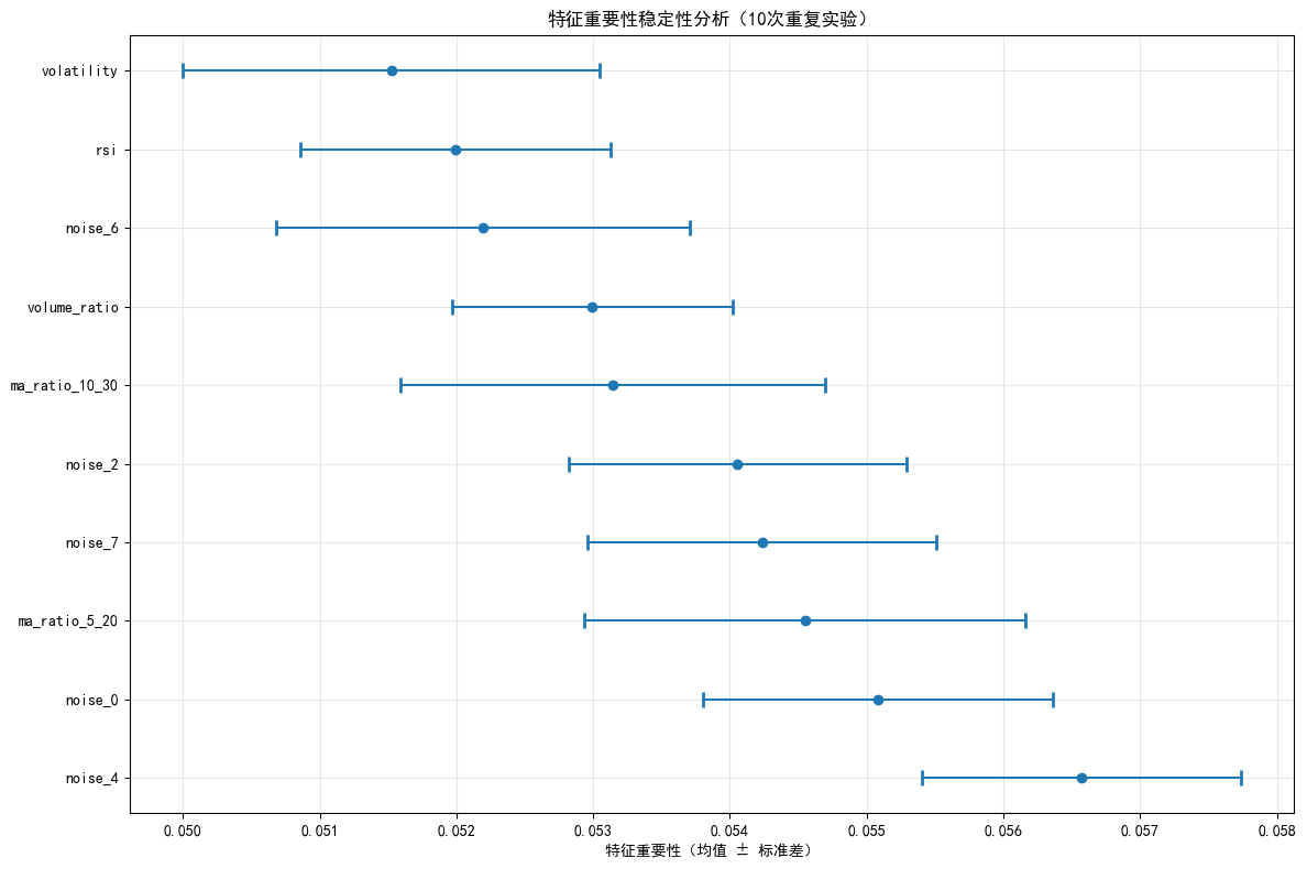
特征重要性稳定性（Top 10）:
       feature  mean_importance      std       cv
       noise_4         0.056572 0.001168 0.020645
       noise_0         0.055084 0.001278 0.023195
 ma_ratio_5_20         0.054549 0.001612 0.029552
       noise_7         0.054236 0.001276 0.023526
       noise_2         0.054053 0.001235 0.022857
ma_ratio_10_30         0.053144 0.001556 0.029281
  volume_ratio         0.052993 0.001025 0.019344
       noise_6         0.052198 0.001513 0.028977
           rsi         0.051992 0.001138 0.021879
    volatility         0.051522 0.001526 0.029617

12. 今日总结

1. 核心概念掌握：

   • Bagging：Bootstrap采样 + 聚合
   • 随机森林：Bagging + 特征随机
   • OOB评估：利用未被采样的样本进行验证
   • 特征重要性：基于不纯度减少或OOB误差

2. 实践成果：

   • 训练了随机森林模型进行涨跌预测
   • 分析了20+个特征的重要性
   • 基于重要性删除了低价值特征
   • 模型性能得到提升

3. 关键参数：

   • n_estimators：树的数量（越大越稳定）
   • max_depth：限制深度（防止过拟合）
   • min_samples_split：分裂所需最小样本数
   • max_features：特征子集大小

4. 随机森林 vs 决策树：

   • 随机森林显著降低过拟合
   • 特征重要性更稳定
   • 需要更多计算资源

5. 注意事项：

   • 随机森林不适合高维稀疏数据
   • 预测速度较慢
   • 可解释性较弱

6. 量化交易应用：

   • 因子选股模型
   • 市场择时信号
   • 风险因子识别

扩展作业

• 作业1：尝试不同的max_features参数，观察对性能的影响
• 作业2：使用RandomForestRegressor预测连续收益率
• 作业3：实现自定义的特征重要性计算（基于OOB误差）
• 作业4：在实际股票数据上测试随机森林策略（使用yfinance）

量化思考

• 随机森林的OOB评分可以作为策略验证的快速参考
• 特征重要性可以帮助筛选有效因子
• 随机森林的"黑箱"特性在合规性要求高的场景需谨慎