多物理场耦合仿真-主题096-不确定性量化与敏感性分析
第096篇:不确定性量化与敏感性分析
摘要
不确定性量化(Uncertainty Quantification, UQ)与敏感性分析(Sensitivity Analysis, SA)是现代科学与工程仿真的核心组成部分。在实际工程问题中,模型输入参数往往存在不确定性,这些不确定性会传播到输出结果中,影响决策的可靠性。本教程系统介绍不确定性量化与敏感性分析的理论基础、数学方法和计算实现。内容涵盖概率统计基础、蒙特卡洛方法、代理模型技术、方差分解方法、Sobol敏感性指数、 Morris筛选方法、多项式混沌展开、高斯过程回归等核心方法。通过六个典型工程案例——结构可靠性分析、热传导不确定性传播、流体动力学敏感性分析、化学反应动力学参数识别、多物理场耦合不确定性量化以及贝叶斯模型校准,展示如何运用Python实现完整的不确定性量化与敏感性分析流程。每个案例均包含详细的数学推导、Python代码实现和可视化分析,帮助读者深入理解不确定性量化在多物理场耦合仿真中的重要性和应用方法。
关键词
不确定性量化,敏感性分析,蒙特卡洛方法,Sobol指数,多项式混沌,高斯过程,贝叶斯校准,方差分解,代理模型,可靠性分析


1. 引言
1.1 不确定性量化的重要性
在科学与工程领域,数学模型和数值仿真已成为理解和预测物理系统行为的重要工具。然而,实际工程问题中存在着各种不确定性来源,这些不确定性会显著影响仿真结果的可靠性和工程决策的准确性。
不确定性的主要来源包括:
-
参数不确定性:材料属性、几何尺寸、边界条件等输入参数往往无法精确测定,存在一定的测量误差或自然变异。
-
模型不确定性:数学模型本身是对物理现实的近似,可能忽略某些物理机制或采用简化假设。
-
数值不确定性:离散化误差、迭代收敛误差、舍入误差等数值计算引入的不确定性。
-
外部不确定性:环境条件、载荷工况等外部因素的不确定性。
不确定性量化(UQ)的目标就是系统地识别、表征和传播这些不确定性,从而评估输出结果的置信区间和可靠性。这对于工程设计优化、风险评估和决策制定具有重要意义。
1.2 敏感性分析的作用
敏感性分析研究输入参数的变化对输出结果的影响程度,帮助识别对系统行为起主导作用的关键参数。通过敏感性分析,可以:
- 识别关键参数:确定哪些参数对输出影响最大,优先进行精确测量或控制
- 简化模型:剔除对输出影响很小的参数,降低模型复杂度
- 指导实验设计:将资源集中在测量关键参数上
- 评估模型稳健性:了解模型对参数扰动的敏感程度
- 支持决策制定:为风险管理和优化设计提供依据
1.3 不确定性量化与敏感性分析的关系
不确定性量化和敏感性分析是紧密相关的两个领域。敏感性分析通常是不确定性量化的前置步骤,用于识别最重要的不确定性来源;而不确定性量化则提供了评估这些不确定性影响的定量方法。
两者的结合使用可以帮助工程师和科学家:
- 理解复杂系统的行为特征
- 评估仿真结果的可信度
- 优化实验和计算资源分配
- 提高工程设计的鲁棒性和可靠性
2. 概率统计基础
2.1 随机变量与概率分布
随机变量是描述不确定性的基本数学工具。根据取值特点,随机变量可分为离散型和连续型两类。
离散型随机变量取有限或可数无限个值,其不确定性由概率质量函数(PMF)描述:
P(X=xi)=pi,i=1,2,…P(X = x_i) = p_i, \quad i = 1, 2, \ldotsP(X=xi)=pi,i=1,2,…
连续型随机变量在实数区间内取值,其不确定性由概率密度函数(PDF)描述:
P(a≤X≤b)=∫abfX(x)dxP(a \leq X \leq b) = \int_a^b f_X(x) dxP(a≤X≤b)=∫abfX(x)dx
累积分布函数(CDF)定义为:
FX(x)=P(X≤x)=∫−∞xfX(t)dtF_X(x) = P(X \leq x) = \int_{-\infty}^x f_X(t) dtFX(x)=P(X≤x)=∫−∞xfX(t)dt
2.2 常用概率分布
**正态分布(高斯分布)**是最常用的连续分布,其概率密度函数为:
f(x)=1σ2πexp(−(x−μ)22σ2)f(x) = \frac{1}{\sigma\sqrt{2\pi}} \exp\left(-\frac{(x-\mu)^2}{2\sigma^2}\right)f(x)=σ2π1exp(−2σ2(x−μ)2)
其中 μ\muμ 为均值,σ\sigmaσ 为标准差。正态分布适用于描述测量误差、材料属性的自然变异等。
均匀分布表示随机变量在区间内等概率取值:
f(x)={1b−a,a≤x≤b0,其他f(x) = \begin{cases} \frac{1}{b-a}, & a \leq x \leq b \\ 0, & \text{其他} \end{cases}f(x)={b−a1,0,a≤x≤b其他
当只知道参数的变化范围而缺乏更多信息时,常采用均匀分布。
对数正态分布适用于描述正值参数,如材料强度、疲劳寿命等:\n
f(x)=1xσ2πexp(−(lnx−μ)22σ2),x>0f(x) = \frac{1}{x\sigma\sqrt{2\pi}} \exp\left(-\frac{(\ln x - \mu)^2}{2\sigma^2}\right), \quad x > 0f(x)=xσ2π1exp(−2σ2(lnx−μ)2),x>0
威布尔分布常用于可靠性分析和寿命预测:
f(x)=kλ(xλ)k−1exp(−(xλ)k),x≥0f(x) = \frac{k}{\lambda}\left(\frac{x}{\lambda}\right)^{k-1} \exp\left(-\left(\frac{x}{\lambda}\right)^k\right), \quad x \geq 0f(x)=λk(λx)k−1exp(−(λx)k),x≥0
其中 kkk 为形状参数,λ\lambdaλ 为尺度参数。
2.3 统计矩与数字特征
随机变量的数字特征提供了不确定性的定量描述:
期望值(均值):
E[X]=μ=∫−∞∞xf(x)dxE[X] = \mu = \int_{-\infty}^{\infty} x f(x) dxE[X]=μ=∫−∞∞xf(x)dx
方差:
Var(X)=σ2=E[(X−μ)2]=∫−∞∞(x−μ)2f(x)dx\text{Var}(X) = \sigma^2 = E[(X-\mu)^2] = \int_{-\infty}^{\infty} (x-\mu)^2 f(x) dxVar(X)=σ2=E[(X−μ)2]=∫−∞∞(x−μ)2f(x)dx
标准差:σ=Var(X)\sigma = \sqrt{\text{Var}(X)}σ=Var(X)
变异系数:CV=σμCV = \frac{\sigma}{\mu}CV=μσ,用于比较不同量级参数的离散程度
偏度:
γ1=E[(X−μ)3]σ3\gamma_1 = \frac{E[(X-\mu)^3]}{\sigma^3}γ1=σ3E[(X−μ)3]
描述分布的不对称性。
峰度:
γ2=E[(X−μ)4]σ4−3\gamma_2 = \frac{E[(X-\mu)^4]}{\sigma^4} - 3γ2=σ4E[(X−μ)4]−3
描述分布尾部的厚重程度。
2.4 多元随机变量与相关性
对于多个随机变量 X1,X2,…,XnX_1, X_2, \ldots, X_nX1,X2,…,Xn,其联合分布描述整体不确定性。
协方差度量两个随机变量的线性相关性:
Cov(X,Y)=E[(X−μX)(Y−μY)]\text{Cov}(X, Y) = E[(X-\mu_X)(Y-\mu_Y)]Cov(X,Y)=E[(X−μX)(Y−μY)]
相关系数:
ρXY=Cov(X,Y)σXσY,−1≤ρXY≤1\rho_{XY} = \frac{\text{Cov}(X, Y)}{\sigma_X \sigma_Y}, \quad -1 \leq \rho_{XY} \leq 1ρXY=σXσYCov(X,Y),−1≤ρXY≤1
协方差矩阵描述多元随机变量的相关性结构:
Σ=[σ12σ12⋯σ1nσ21σ22⋯σ2n⋮⋮⋱⋮σn1σn2⋯σn2]\mathbf{\Sigma} = \begin{bmatrix} \sigma_1^2 & \sigma_{12} & \cdots & \sigma_{1n} \\ \sigma_{21} & \sigma_2^2 & \cdots & \sigma_{2n} \\ \vdots & \vdots & \ddots & \vdots \\ \sigma_{n1} & \sigma_{n2} & \cdots & \sigma_n^2 \end{bmatrix}Σ= σ12σ21⋮σn1σ12σ22⋮σn2⋯⋯⋱⋯σ1nσ2n⋮σn2
对于相关随机变量的采样,常用的方法是Cholesky分解:
X=μ+LZ\mathbf{X} = \mathbf{\mu} + \mathbf{L}\mathbf{Z}X=μ+LZ
其中 L\mathbf{L}L 是协方差矩阵的下三角分解(Σ=LLT\mathbf{\Sigma} = \mathbf{L}\mathbf{L}^TΣ=LLT),Z\mathbf{Z}Z 是独立标准正态随机向量。
3. 不确定性传播方法
3.1 蒙特卡洛方法
蒙特卡洛方法是不确定性量化中最通用和鲁棒的方法。其基本思想是通过大量随机采样来估计输出统计量。
基本步骤:
-
输入采样:根据输入参数的概率分布,生成 NNN 组随机样本 x(1),x(2),…,x(N)\mathbf{x}^{(1)}, \mathbf{x}^{(2)}, \ldots, \mathbf{x}^{(N)}x(1),x(2),…,x(N)
-
模型求解:对每个样本运行仿真模型,获得输出 y(i)=f(x(i))y^{(i)} = f(\mathbf{x}^{(i)})y(i)=f(x(i))
-
统计分析:基于输出样本估计统计量
统计量估计:
均值估计:μ^Y=1N∑i=1Ny(i)\hat{\mu}_Y = \frac{1}{N}\sum_{i=1}^N y^{(i)}μ^Y=N1∑i=1Ny(i)
方差估计:σ^Y2=1N−1∑i=1N(y(i)−μ^Y)2\hat{\sigma}_Y^2 = \frac{1}{N-1}\sum_{i=1}^N (y^{(i)} - \hat{\mu}_Y)^2σ^Y2=N−11∑i=1N(y(i)−μ^Y)2
概率估计:P(Y≤y0)≈1N∑i=1NI(y(i)≤y0)P(Y \leq y_0) \approx \frac{1}{N}\sum_{i=1}^N \mathbb{I}(y^{(i)} \leq y_0)P(Y≤y0)≈N1∑i=1NI(y(i)≤y0)
蒙特卡洛方法的收敛速度为 O(1/N)O(1/\sqrt{N})O(1/N),即样本量增加4倍,精度提高1倍。虽然收敛速度较慢,但蒙特卡洛方法不依赖于模型的具体形式,适用于高度非线性和复杂模型。
3.2 拉丁超立方采样
拉丁超立方采样(LHS)是一种分层采样技术,可以用更少的样本获得更好的统计估计。
基本原理:
将每个输入变量的分布分成 NNN 个等概率区间,在每个区间中随机抽取一个样本,并确保每个区间只有一个样本。这种方法保证了样本在输入空间中的均匀分布。
优势:
- 样本覆盖整个输入空间
- 方差通常小于简单随机采样
- 对于光滑函数,收敛速度更快
3.3 泰勒级数展开法
对于小不确定性问题,可以使用泰勒级数展开来近似不确定性传播。
设 Y=f(X)Y = f(X)Y=f(X),在均值 μX\mu_XμX 处展开:
Y≈f(μX)+f′(μX)(X−μX)+12f′′(μX)(X−μX)2Y \approx f(\mu_X) + f'(\mu_X)(X - \mu_X) + \frac{1}{2}f''(\mu_X)(X - \mu_X)^2Y≈f(μX)+f′(μX)(X−μX)+21f′′(μX)(X−μX)2
一阶近似:
μY≈f(μX)\mu_Y \approx f(\mu_X)μY≈f(μX)
σY2≈[f′(μX)]2σX2\sigma_Y^2 \approx [f'(\mu_X)]^2 \sigma_X^2σY2≈[f′(μX)]2σX2
二阶近似:
μY≈f(μX)+12f′′(μX)σX2\mu_Y \approx f(\mu_X) + \frac{1}{2}f''(\mu_X)\sigma_X^2μY≈f(μX)+21f′′(μX)σX2
泰勒级数方法计算效率高,但仅适用于小不确定性和光滑函数。
3.4 点估计法
点估计法通过选择特定的样本点来估计输出统计量,避免了大量采样。
Rosenblueth方法:
对于 nnn 个正态分布输入变量,使用 2n2^n2n 个采样点(每个变量取 μ±σ\mu \pm \sigmaμ±σ)。
Harr方法:
使用 2n2n2n 个采样点,通过特征值分解考虑变量相关性。
点估计法计算效率高,但对于高度非线性模型可能精度不足。
4. 敏感性分析方法
4.1 局部敏感性分析
局部敏感性分析研究输入参数在名义值附近的小变化对输出的影响。
偏导数法:
Si=∂Y∂Xi∣X=μS_i = \frac{\partial Y}{\partial X_i}\bigg|_{\mathbf{X}=\mathbf{\mu}}Si=∂Xi∂Y X=μ
标准化敏感性系数:
Si∗=∂Y∂Xi⋅σXiσYS_i^* = \frac{\partial Y}{\partial X_i} \cdot \frac{\sigma_{X_i}}{\sigma_Y}Si∗=∂Xi∂Y⋅σYσXi
局部敏感性分析计算简单,但只能反映参数在名义值附近的敏感性,无法捕捉参数间的交互作用。
4.2 全局敏感性分析
全局敏感性分析考虑参数在整个变化范围内的影响,以及参数间的交互作用。
方差分解方法:
将输出方差分解为各输入参数及其交互作用的贡献:
Var(Y)=∑iVi+∑i<jVij+∑i<j<kVijk+⋯+V12⋯n\text{Var}(Y) = \sum_i V_i + \sum_{i<j} V_{ij} + \sum_{i<j<k} V_{ijk} + \cdots + V_{12\cdots n}Var(Y)=i∑Vi+i<j∑Vij+i<j<k∑Vijk+⋯+V12⋯n
其中:
- Vi=VarXi(EX∼i[Y∣Xi])V_i = \text{Var}_{X_i}(E_{\mathbf{X}_{\sim i}}[Y|X_i])Vi=VarXi(EX∼i[Y∣Xi]) 是参数 XiX_iXi 的主效应
- Vij=VarXi,Xj(EX∼ij[Y∣Xi,Xj])−Vi−VjV_{ij} = \text{Var}_{X_i,X_j}(E_{\mathbf{X}_{\sim ij}}[Y|X_i,X_j]) - V_i - V_jVij=VarXi,Xj(EX∼ij[Y∣Xi,Xj])−Vi−Vj 是交互效应
4.3 Sobol敏感性指数
Sobol指数是基于方差分解的全局敏感性指标。
一阶Sobol指数:
Si=ViVar(Y)S_i = \frac{V_i}{\text{Var}(Y)}Si=Var(Y)Vi
表示参数 XiX_iXi 单独对输出方差的贡献比例。
总效应指数:
STi=EX∼i[VarXi(Y∣X∼i)]Var(Y)=1−VarX∼i(EXi[Y∣X∼i])Var(Y)S_{Ti} = \frac{E_{\mathbf{X}_{\sim i}}[\text{Var}_{X_i}(Y|\mathbf{X}_{\sim i})]}{\text{Var}(Y)} = 1 - \frac{\text{Var}_{\mathbf{X}_{\sim i}}(E_{X_i}[Y|\mathbf{X}_{\sim i}])}{\text{Var}(Y)}STi=Var(Y)EX∼i[VarXi(Y∣X∼i)]=1−Var(Y)VarX∼i(EXi[Y∣X∼i])
表示参数 XiX_iXi 及其与其他参数的所有交互作用对输出方差的总贡献。
二阶Sobol指数:
Sij=VijVar(Y)S_{ij} = \frac{V_{ij}}{\text{Var}(Y)}Sij=Var(Y)Vij
表示参数 XiX_iXi 和 XjX_jXj 的交互效应对输出方差的贡献。
Sobol指数满足:0≤Si≤STi≤10 \leq S_i \leq S_{Ti} \leq 10≤Si≤STi≤1,且 ∑iSi≤1\sum_i S_i \leq 1∑iSi≤1。
Sobol指数的计算:
使用蒙特卡洛方法估计Sobol指数需要两组样本矩阵 A\mathbf{A}A 和 B\mathbf{B}B,以及混合矩阵 AB(i)\mathbf{A}_B^{(i)}AB(i)(将 A\mathbf{A}A 的第 iii 列替换为 B\mathbf{B}B 的第 iii 列)。
Vi=1N∑j=1Nf(B)j[f(AB(i))j−f(A)j]V_i = \frac{1}{N}\sum_{j=1}^N f(\mathbf{B})_j [f(\mathbf{A}_B^{(i)})_j - f(\mathbf{A})_j]Vi=N1j=1∑Nf(B)j[f(AB(i))j−f(A)j]
Var(Y)=1N∑j=1Nf(A)j2−(1N∑j=1Nf(A)j)2\text{Var}(Y) = \frac{1}{N}\sum_{j=1}^N f(\mathbf{A})_j^2 - \left(\frac{1}{N}\sum_{j=1}^N f(\mathbf{A})_j\right)^2Var(Y)=N1j=1∑Nf(A)j2−(N1j=1∑Nf(A)j)2
4.4 Morris筛选方法
Morris方法是一种计算效率高的定性敏感性分析方法,用于筛选重要参数。
基本思想:
通过计算基本效应(Elementary Effects)来评估参数的敏感性:
EEi=f(x1,…,xi+Δ,…,xn)−f(x1,…,xi,…,xn)ΔEE_i = \frac{f(x_1, \ldots, x_i + \Delta, \ldots, x_n) - f(x_1, \ldots, x_i, \ldots, x_n)}{\Delta}EEi=Δf(x1,…,xi+Δ,…,xn)−f(x1,…,xi,…,xn)
统计量:
- 基本效应的均值 μi\mu_iμi:表示参数的总体重要性
- 基本效应的标准差 σi\sigma_iσi:表示参数的交互作用程度和非线性程度
解释:
- 高 μi\mu_iμi:参数对输出有显著线性影响
- 高 σi\sigma_iσi:参数具有强非线性效应或与其他参数有交互作用
- 低 μi\mu_iμi 和 σi\sigma_iσi:参数对输出影响很小,可以固定
Morris方法计算成本低(只需要 O(n)O(n)O(n) 次模型评估),适合参数众多的初步筛选。
4.5 基于回归的敏感性分析
当有足够的样本数据时,可以使用回归分析来评估敏感性。
标准化回归系数(SRC):
SRCi=βi⋅σXiσYSRC_i = \beta_i \cdot \frac{\sigma_{X_i}}{\sigma_Y}SRCi=βi⋅σYσXi
其中 βi\beta_iβi 是线性回归系数。SRCi2SRC_i^2SRCi2 表示参数 XiX_iXi 对输出方差的线性贡献。
偏相关系数(PCC):
在控制其他变量影响后,度量 XiX_iXi 与 YYY 的相关性。
基于回归的方法简单直观,但仅适用于近似线性的模型。
5. 代理模型方法
5.1 代理模型的概念
代理模型(Surrogate Model)或元模型(Metamodel)是计算模型的近似表示,可以用较少的计算成本来近似原模型的输入-输出关系。
代理模型的优势:
- 大幅降低计算成本
- 支持快速不确定性传播
- 便于敏感性分析
- 可用于优化设计
常用代理模型类型:
- 多项式响应面(RSM)
- 克里金模型(Kriging)
- 高斯过程回归(GPR)
- 径向基函数(RBF)
- 神经网络
- 多项式混沌展开(PCE)
5.2 多项式响应面方法
响应面方法使用低阶多项式来近似模型响应。
一阶模型:
Y^=β0+∑i=1nβiXi\hat{Y} = \beta_0 + \sum_{i=1}^n \beta_i X_iY^=β0+i=1∑nβiXi
二阶模型:
Y^=β0+∑i=1nβiXi+∑i=1nβiiXi2+∑i<jβijXiXj\hat{Y} = \beta_0 + \sum_{i=1}^n \beta_i X_i + \sum_{i=1}^n \beta_{ii} X_i^2 + \sum_{i<j} \beta_{ij} X_i X_jY^=β0+i=1∑nβiXi+i=1∑nβiiXi2+i<j∑βijXiXj
系数估计:
使用最小二乘法估计多项式系数:
β=(XTX)−1XTY\mathbf{\beta} = (\mathbf{X}^T\mathbf{X})^{-1}\mathbf{X}^T\mathbf{Y}β=(XTX)−1XTY
其中 X\mathbf{X}X 是设计矩阵,包含样本点的多项式基函数值。
5.3 高斯过程回归
高斯过程回归是一种强大的非参数代理模型方法,提供了预测值和不确定性估计。
高斯过程定义:
高斯过程是随机变量的集合,其中任意有限个随机变量的联合分布都是多元高斯分布。由均值函数 m(x)m(\mathbf{x})m(x) 和协方差函数(核函数)k(x,x′)k(\mathbf{x}, \mathbf{x}')k(x,x′) 完全确定。
常用核函数:
平方指数核(RBF):
k(x,x′)=σf2exp(−12∑i=1d(xi−xi′)2li2)k(\mathbf{x}, \mathbf{x}') = \sigma_f^2 \exp\left(-\frac{1}{2}\sum_{i=1}^d \frac{(x_i - x_i')^2}{l_i^2}\right)k(x,x′)=σf2exp(−21i=1∑dli2(xi−xi′)2)
Matérn核:
k(x,x′)=σf221−νΓ(ν)(2νrl)νKν(2νrl)k(\mathbf{x}, \mathbf{x}') = \sigma_f^2 \frac{2^{1-\nu}}{\Gamma(\nu)}\left(\frac{\sqrt{2\nu}r}{l}\right)^\nu K_\nu\left(\frac{\sqrt{2\nu}r}{l}\right)k(x,x′)=σf2Γ(ν)21−ν(l2νr)νKν(l2νr)
其中 r=∣∣x−x′∣∣r = ||\mathbf{x} - \mathbf{x}'||r=∣∣x−x′∣∣,KνK_\nuKν 是修正贝塞尔函数。
预测:
给定训练数据 (X,y)(\mathbf{X}, \mathbf{y})(X,y),对于新输入 x∗\mathbf{x}^*x∗,预测分布为:
p(y∗∣x∗,X,y)=N(μ(x∗),σ2(x∗))p(y^*|\mathbf{x}^*, \mathbf{X}, \mathbf{y}) = \mathcal{N}(\mu(\mathbf{x}^*), \sigma^2(\mathbf{x}^*))p(y∗∣x∗,X,y)=N(μ(x∗),σ2(x∗))
其中:
μ(x∗)=k∗K−1y\mu(\mathbf{x}^*) = \mathbf{k}^* \mathbf{K}^{-1} \mathbf{y}μ(x∗)=k∗K−1y
σ2(x∗)=k(x∗,x∗)−k∗K−1k∗T\sigma^2(\mathbf{x}^*) = k(\mathbf{x}^*, \mathbf{x}^*) - \mathbf{k}^* \mathbf{K}^{-1} \mathbf{k}^{*T}σ2(x∗)=k(x∗,x∗)−k∗K−1k∗T
高斯过程回归的优点是能够提供预测不确定性估计,适合小样本学习。
5.4 多项式混沌展开
多项式混沌展开(Polynomial Chaos Expansion, PCE)使用正交多项式基来展开随机输出。
广义PCE:
Y(ξ)=∑α∈AyαΨα(ξ)Y(\mathbf{\xi}) = \sum_{\mathbf{\alpha} \in \mathcal{A}} y_{\mathbf{\alpha}} \Psi_{\mathbf{\alpha}}(\mathbf{\xi})Y(ξ)=α∈A∑yαΨα(ξ)
其中 ξ\mathbf{\xi}ξ 是标准随机变量,Ψα\Psi_{\mathbf{\alpha}}Ψα 是正交多项式,yαy_{\mathbf{\alpha}}yα 是展开系数。
多项式选择:
- 正态分布 →\rightarrow→ Hermite多项式
- 均匀分布 →\rightarrow→ Legendre多项式
- 伽马分布 →\rightarrow→ Laguerre多项式
- 贝塔分布 →\rightarrow→ Jacobi多项式
系数计算:
可以使用投影法或回归法计算展开系数。投影法利用正交性:
yα=E[YΨα]E[Ψα2]y_{\mathbf{\alpha}} = \frac{E[Y\Psi_{\mathbf{\alpha}}]}{E[\Psi_{\mathbf{\alpha}}^2]}yα=E[Ψα2]E[YΨα]
统计量提取:
PCE展开后,统计量可以直接从系数计算:
μY=y0\mu_Y = y_0μY=y0
σY2=∑α≠0yα2E[Ψα2]\sigma_Y^2 = \sum_{\mathbf{\alpha} \neq 0} y_{\mathbf{\alpha}}^2 E[\Psi_{\mathbf{\alpha}}^2]σY2=α=0∑yα2E[Ψα2]
Sobol指数也可以直接从PCE系数计算,无需额外采样。
6. 贝叶斯方法
6.1 贝叶斯推断基础
贝叶斯方法提供了一种系统的方式来更新对参数的认知。
贝叶斯定理:
p(θ∣d)=p(d∣θ)p(θ)p(d)p(\mathbf{\theta}|\mathbf{d}) = \frac{p(\mathbf{d}|\mathbf{\theta})p(\mathbf{\theta})}{p(\mathbf{d})}p(θ∣d)=p(d)p(d∣θ)p(θ)
其中:
- p(θ)p(\mathbf{\theta})p(θ):先验分布,表示观测数据前的参数认知
- p(d∣θ)p(\mathbf{d}|\mathbf{\theta})p(d∣θ):似然函数,表示给定参数下观测数据的概率
- p(θ∣d)p(\mathbf{\theta}|\mathbf{d})p(θ∣d):后验分布,表示观测数据后的参数认知
- p(d)p(\mathbf{d})p(d):证据,用于归一化
6.2 马尔可夫链蒙特卡洛
马尔可夫链蒙特卡洛(MCMC)方法用于从复杂后验分布中采样。
Metropolis-Hastings算法:
- 初始化 θ(0)\mathbf{\theta}^{(0)}θ(0)
- 对于 t=1,2,…,Nt = 1, 2, \ldots, Nt=1,2,…,N:
- 从提议分布 q(θ∗∣θ(t−1))q(\mathbf{\theta}^*|\mathbf{\theta}^{(t-1)})q(θ∗∣θ(t−1)) 采样候选点
- 计算接受概率:α=min(1,p(θ∗∣d)q(θ(t−1)∣θ∗)p(θ(t−1)∣d)q(θ∗∣θ(t−1)))\alpha = \min\left(1, \frac{p(\mathbf{\theta}^*|\mathbf{d})q(\mathbf{\theta}^{(t-1)}|\mathbf{\theta}^*)}{p(\mathbf{\theta}^{(t-1)}|\mathbf{d})q(\mathbf{\theta}^*|\mathbf{\theta}^{(t-1)})}\right)α=min(1,p(θ(t−1)∣d)q(θ∗∣θ(t−1))p(θ∗∣d)q(θ(t−1)∣θ∗))
- 以概率 α\alphaα 接受候选点,否则保持当前值
Gibbs采样:
当条件分布容易采样时,依次从每个参数的条件分布采样。
6.3 贝叶斯模型校准
贝叶斯校准用于结合仿真模型和实验数据来估计模型参数。
模型形式:
di=f(xi;θ)+ϵid_i = f(\mathbf{x}_i; \mathbf{\theta}) + \epsilon_idi=f(xi;θ)+ϵi
其中 ϵi\epsilon_iϵi 是观测误差,通常假设为 N(0,σ2)\mathcal{N}(0, \sigma^2)N(0,σ2)。
似然函数:
p(d∣θ)=∏i=1n12πσexp(−(di−f(xi;θ))22σ2)p(\mathbf{d}|\mathbf{\theta}) = \prod_{i=1}^n \frac{1}{\sqrt{2\pi}\sigma} \exp\left(-\frac{(d_i - f(\mathbf{x}_i; \mathbf{\theta}))^2}{2\sigma^2}\right)p(d∣θ)=i=1∏n2πσ1exp(−2σ2(di−f(xi;θ))2)
后验采样:
使用MCMC从后验分布采样,获得参数的分布估计。
7. Python仿真案例
7.1 案例1:结构可靠性分析
本案例演示如何使用蒙特卡洛方法进行结构可靠性分析。
#!/usr/bin/env python3
# -*- coding: utf-8 -*-
"""
案例1:结构可靠性分析
使用蒙特卡洛方法计算悬臂梁的失效概率
"""

import numpy as np
import matplotlib
matplotlib.use('Agg')
import matplotlib.pyplot as plt
from scipy import stats
import warnings
warnings.filterwarnings('ignore')

plt.rcParams['font.sans-serif'] = ['SimHei', 'DejaVu Sans']
plt.rcParams['axes.unicode_minus'] = False

print("="*70)
print("案例1:结构可靠性分析")
print("="*70)

# 悬臂梁参数(带不确定性)
# 长度 L ~ N(2.0, 0.02) m
# 宽度 b ~ N(0.1, 0.002) m
# 高度 h ~ N(0.2, 0.004) m
# 载荷 P ~ N(10000, 1000) N
# 屈服强度 sigma_y ~ N(250e6, 25e6) Pa

np.random.seed(42)
n_samples = 100000

# 生成随机样本
L = np.random.normal(2.0, 0.02, n_samples)
b = np.random.normal(0.1, 0.002, n_samples)
h = np.random.normal(0.2, 0.004, n_samples)
P = np.random.normal(10000, 1000, n_samples)
sigma_y = np.random.normal(250e6, 25e6, n_samples)

# 计算截面惯性矩
I = b * h**3 / 12

# 计算最大弯矩(悬臂梁端部受集中力)
M_max = P * L

# 计算最大应力
sigma_max = M_max * h / (2 * I)

# 计算安全裕度
g = sigma_y - sigma_max

# 计算失效概率
p_f = np.sum(g < 0) / n_samples
print(f"\n蒙特卡洛仿真结果(N={n_samples}):")
print(f"失效概率 Pf = {p_f:.6f}")
print(f"可靠性指数 beta = {-stats.norm.ppf(p_f):.4f}")

# 统计结果
print(f"\n最大应力统计:")
print(f"  均值 = {np.mean(sigma_max)/1e6:.2f} MPa")
print(f"  标准差 = {np.std(sigma_max)/1e6:.2f} MPa")
print(f"  最大值 = {np.max(sigma_max)/1e6:.2f} MPa")

print(f"\n安全裕度统计:")
print(f"  均值 = {np.mean(g)/1e6:.2f} MPa")
print(f"  标准差 = {np.std(g)/1e6:.2f} MPa")
print(f"  最小值 = {np.min(g)/1e6:.2f} MPa")

# 可视化
fig, axes = plt.subplots(2, 2, figsize=(14, 10))

# 图1:应力分布
ax1 = axes[0, 0]
ax1.hist(sigma_max/1e6, bins=50, density=True, alpha=0.7, color='blue', edgecolor='black')
ax1.axvline(x=np.mean(sigma_y)/1e6, color='red', linestyle='--', linewidth=2, label='Yield Strength')
ax1.set_xlabel('Maximum Stress (MPa)')
ax1.set_ylabel('Probability Density')
ax1.set_title('Stress Distribution')
ax1.legend()
ax1.grid(True, alpha=0.3)

# 图2:安全裕度分布
ax2 = axes[0, 1]
ax2.hist(g/1e6, bins=50, density=True, alpha=0.7, color='green', edgecolor='black')
ax2.axvline(x=0, color='red', linestyle='--', linewidth=2, label='Failure Limit')
ax2.set_xlabel('Safety Margin (MPa)')
ax2.set_ylabel('Probability Density')
ax2.set_title('Safety Margin Distribution')
ax2.legend()
ax2.grid(True, alpha=0.3)

# 图3:散点图 - 载荷vs应力
ax3 = axes[1, 0]
scatter = ax3.scatter(P[::100]/1000, sigma_max[::100]/1e6, c=g[::100]/1e6,
                      cmap='RdYlGn', alpha=0.6, s=10)
ax3.axhline(y=np.mean(sigma_y)/1e6, color='red', linestyle='--', linewidth=2)
ax3.set_xlabel('Load (kN)')
ax3.set_ylabel('Maximum Stress (MPa)')
ax3.set_title('Load vs Stress')
plt.colorbar(scatter, ax=ax3, label='Safety Margin (MPa)')
ax3.grid(True, alpha=0.3)

# 图4:收敛性分析
ax4 = axes[1, 1]
sample_sizes = np.logspace(2, 5, 20).astype(int)
pf_convergence = []
for n in sample_sizes:
    pf_n = np.sum(g[:n] < 0) / n
    pf_convergence.append(pf_n)

ax4.semilogx(sample_sizes, pf_convergence, 'b-o', linewidth=2, markersize=6)
ax4.axhline(y=p_f, color='red', linestyle='--', linewidth=2, label=f'Final Pf={p_f:.6f}')
ax4.set_xlabel('Number of Samples')
ax4.set_ylabel('Failure Probability')
ax4.set_title('Convergence Analysis')
ax4.legend()
ax4.grid(True, alpha=0.3)

plt.tight_layout()
plt.savefig('case1_structural_reliability.png', dpi=150)
print("\n案例1完成!")
7.2 案例2:热传导不确定性传播
本案例演示不确定性在热传导问题中的传播。
#!/usr/bin/env python3
# -*- coding: utf-8 -*-
"""
案例2:热传导不确定性传播
分析材料参数不确定性对温度场的影响
"""

import numpy as np
import matplotlib
matplotlib.use('Agg')
import matplotlib.pyplot as plt
from scipy.sparse import diags
from scipy.sparse.linalg import spsolve
import warnings
warnings.filterwarnings('ignore')

plt.rcParams['font.sans-serif'] = ['SimHei', 'DejaVu Sans']
plt.rcParams['axes.unicode_minus'] = False

print("\n" + "="*70)
print("案例2:热传导不确定性传播")
print("="*70)

# 问题设置
L = 1.0  # 板长度 (m)
T_left = 100.0  # 左边界温度 (°C)
T_right = 0.0   # 右边界温度 (°C)
n_nodes = 50    # 网格节点数

# 不确定性参数
# 导热系数 k ~ N(50, 5) W/(m·K)
# 热源强度 q ~ N(1000, 100) W/m³

np.random.seed(123)
n_samples = 5000

# 生成随机样本
k_samples = np.random.normal(50, 5, n_samples)
q_samples = np.random.normal(1000, 100, n_samples)

# 求解确定性热传导方程
def solve_heat_conduction(k, q, n_nodes=50):
    """求解一维稳态热传导方程"""
    x = np.linspace(0, L, n_nodes)
    dx = L / (n_nodes - 1)

    # 构建刚度矩阵
    main_diag = np.full(n_nodes, 2 * k / dx)
    off_diag = np.full(n_nodes - 1, -k / dx)

    # 边界条件
    main_diag[0] = 1.0
    main_diag[-1] = 1.0
    off_diag[0] = 0.0
    off_diag[-1] = 0.0

    A = diags([off_diag, main_diag, off_diag], [-1, 0, 1], format='csr')

    # 右端项
    b = np.full(n_nodes, q * dx)
    b[0] = T_left
    b[-1] = T_right

    # 求解
    T = spsolve(A, b)

    return x, T

# 蒙特卡洛仿真
print("\n进行蒙特卡洛仿真...")
x = np.linspace(0, L, n_nodes)
T_all = np.zeros((n_samples, n_nodes))

for i in range(n_samples):
    _, T_all[i, :] = solve_heat_conduction(k_samples[i], q_samples[i], n_nodes)

# 统计分析
T_mean = np.mean(T_all, axis=0)
T_std = np.std(T_all, axis=0)
T_p5 = np.percentile(T_all, 5, axis=0)
T_p95 = np.percentile(T_all, 95, axis=0)

print(f"\n温度场统计(x=L/2处):")
print(f"  均值 = {T_mean[n_nodes//2]:.2f} °C")
print(f"  标准差 = {T_std[n_nodes//2]:.2f} °C")
print(f"  95%置信区间 = [{T_p5[n_nodes//2]:.2f}, {T_p95[n_nodes//2]:.2f}] °C")

# 可视化
fig, axes = plt.subplots(2, 2, figsize=(14, 10))

# 图1:温度分布(均值和置信区间)
ax1 = axes[0, 0]
ax1.fill_between(x, T_p5, T_p95, alpha=0.3, color='blue', label='90% Confidence Interval')
ax1.plot(x, T_mean, 'b-', linewidth=2, label='Mean')
ax1.set_xlabel('Position (m)')
ax1.set_ylabel('Temperature (°C)')
ax1.set_title('Temperature Distribution with Uncertainty')
ax1.legend()
ax1.grid(True, alpha=0.3)

# 图2:温度标准差分布
ax2 = axes[0, 1]
ax2.plot(x, T_std, 'r-', linewidth=2)
ax2.set_xlabel('Position (m)')
ax2.set_ylabel('Standard Deviation (°C)')
ax2.set_title('Temperature Uncertainty Distribution')
ax2.grid(True, alpha=0.3)

# 图3:特定位置的温度分布
ax3 = axes[1, 0]
mid_idx = n_nodes // 2
ax3.hist(T_all[:, mid_idx], bins=50, density=True, alpha=0.7, color='green', edgecolor='black')
ax3.axvline(x=T_mean[mid_idx], color='red', linestyle='--', linewidth=2, label=f'Mean={T_mean[mid_idx]:.1f}°C')
ax3.set_xlabel('Temperature at x=L/2 (°C)')
ax3.set_ylabel('Probability Density')
ax3.set_title('Temperature Distribution at Midpoint')
ax3.legend()
ax3.grid(True, alpha=0.3)

# 图4:相关系数分析
ax4 = axes[1, 1]
# 计算各参数与中心温度的相关系数
corr_k = np.corrcoef(k_samples, T_all[:, mid_idx])[0, 1]
corr_q = np.corrcoef(q_samples, T_all[:, mid_idx])[0, 1]

correlations = [corr_k, corr_q]
params = ['Thermal Conductivity k', 'Heat Source q']
colors = ['blue', 'red']

bars = ax4.barh(params, correlations, color=colors, alpha=0.7)
ax4.set_xlabel('Correlation Coefficient')
ax4.set_title('Parameter Correlation with Temperature')
ax4.set_xlim(-1, 1)
ax4.grid(True, alpha=0.3, axis='x')

for bar, val in zip(bars, correlations):
    ax4.text(val + 0.05 if val > 0 else val - 0.05, bar.get_y() + bar.get_height()/2,
             f'{val:.3f}', ha='left' if val > 0 else 'right', va='center')

plt.tight_layout()
plt.savefig('case2_heat_uncertainty.png', dpi=150)
print("\n案例2完成!")
7.3 案例3:Sobol敏感性分析
本案例演示如何使用Sobol方法进行全局敏感性分析。
#!/usr/bin/env python3
# -*- coding: utf-8 -*-
"""
案例3:Sobol敏感性分析
使用Sobol指数分析Ishigami函数的全局敏感性
"""

import numpy as np
import matplotlib
matplotlib.use('Agg')
import matplotlib.pyplot as plt
import warnings
warnings.filterwarnings('ignore')

plt.rcParams['font.sans-serif'] = ['SimHei', 'DejaVu Sans']
plt.rcParams['axes.unicode_minus'] = False

print("\n" + "="*70)
print("案例3:Sobol敏感性分析")
print("="*70)

# Ishigami函数 - 经典的敏感性分析测试函数
def ishigami(x):
    """
    Ishigami函数:
    f(x) = sin(x1) + a*sin(x2)^2 + b*x3^4*sin(x1)
    其中 x_i ~ U(-π, π)
    解析解:
    S1 = 0.3139, S2 = 0.4424, S3 = 0.0
    ST1 = 0.5576, ST2 = 0.4424, ST3 = 0.2437
    """
    a = 7
    b = 0.1
    return np.sin(x[:, 0]) + a * np.sin(x[:, 1])**2 + b * x[:, 2]**4 * np.sin(x[:, 0])

def sobol_indices(func, n_samples, n_params):
    """
    使用Saltelli方法估计Sobol指数
    """
    # 生成两个独立的样本矩阵
    np.random.seed(42)
    A = np.random.uniform(-np.pi, np.pi, (n_samples, n_params))
    B = np.random.uniform(-np.pi, np.pi, (n_samples, n_params))

    # 计算函数输出
    f_A = func(A)
    f_B = func(B)

    # 总方差估计
    total_var = np.var(np.concatenate([f_A, f_B]))

    # 一阶Sobol指数
    S1 = np.zeros(n_params)
    ST = np.zeros(n_params)

    for i in range(n_params):
        # 创建混合矩阵 A_B_i
        A_B = A.copy()
        A_B[:, i] = B[:, i]
        f_A_B = func(A_B)

        # 一阶效应
        S1[i] = np.mean(f_B * (f_A_B - f_A)) / total_var

        # 总效应
        ST[i] = 0.5 * np.mean((f_A - f_A_B)**2) / total_var

    return S1, ST, total_var

# 运行Sobol分析
print("\n进行Sobol敏感性分析...")
n_samples = 10000
n_params = 3

S1, ST, total_var = sobol_indices(ishigami, n_samples, n_params)

print(f"\nSobol指数分析结果(N={n_samples}):")
print(f"总方差 = {total_var:.4f}")
print("\n一阶Sobol指数 S1:")
for i in range(n_params):
    print(f"  S1[{i+1}] = {S1[i]:.4f}")

print("\n总效应指数 ST:")
for i in range(n_params):
    print(f"  ST[{i+1}] = {ST[i]:.4f}")

print("\n解析解参考:")
print("  S1 = [0.3139, 0.4424, 0.0000]")
print("  ST = [0.5576, 0.4424, 0.2437]")

# Morris筛选分析
def morris_analysis(func, n_params, n_trajectories=100, delta=0.1):
    """
    Morris筛选方法
    """
    np.random.seed(123)

    elementary_effects = [[] for _ in range(n_params)]

    for _ in range(n_trajectories):
        # 随机选择基准点
        x_base = np.random.uniform(-np.pi, np.pi, n_params)

        for i in range(n_params):
            x_plus = x_base.copy()
            x_minus = x_base.copy()

            x_plus[i] += delta
            x_minus[i] -= delta

            # 确保在边界内
            x_plus[i] = np.clip(x_plus[i], -np.pi, np.pi)
            x_minus[i] = np.clip(x_minus[i], -np.pi, np.pi)

            ee = (func(x_plus.reshape(1, -1)) - func(x_minus.reshape(1, -1))) / (2 * delta)
            elementary_effects[i].append(ee[0])

    # 计算统计量
    mu = np.array([np.mean(ees) for ees in elementary_effects])
    sigma = np.array([np.std(ees) for ees in elementary_effects])

    return mu, sigma

print("\n进行Morris筛选分析...")
mu, sigma = morris_analysis(ishigami, n_params, n_trajectories=200)

print("\nMorris筛选结果:")
for i in range(n_params):
    print(f"  参数{i+1}: μ = {mu[i]:.4f}, σ = {sigma[i]:.4f}")

# 可视化
fig, axes = plt.subplots(2, 2, figsize=(14, 10))

# 图1:Sobol指数对比
ax1 = axes[0, 0]
x_pos = np.arange(n_params)
width = 0.35

bars1 = ax1.bar(x_pos - width/2, S1, width, label='First-order S1', color='blue', alpha=0.7)
bars2 = ax1.bar(x_pos + width/2, ST, width, label='Total-effect ST', color='red', alpha=0.7)

ax1.set_xlabel('Parameter')
ax1.set_ylabel('Sobol Index')
ax1.set_title('Sobol Sensitivity Indices')
ax1.set_xticks(x_pos)
ax1.set_xticklabels([f'x{i+1}' for i in range(n_params)])
ax1.legend()
ax1.grid(True, alpha=0.3, axis='y')

# 添加数值标签
for bar in bars1:
    height = bar.get_height()
    ax1.text(bar.get_x() + bar.get_width()/2., height,
             f'{height:.3f}', ha='center', va='bottom', fontsize=9)
for bar in bars2:
    height = bar.get_height()
    ax1.text(bar.get_x() + bar.get_width()/2., height,
             f'{height:.3f}', ha='center', va='bottom', fontsize=9)

# 图2:Morris筛选图
ax2 = axes[0, 1]
ax2.scatter(mu, sigma, s=200, c=['blue', 'green', 'red'], alpha=0.7, edgecolors='black')
for i in range(n_params):
    ax2.annotate(f'x{i+1}', (mu[i], sigma[i]), xytext=(5, 5),
                textcoords='offset points', fontsize=12)
ax2.set_xlabel('μ (Mean of Elementary Effects)')
ax2.set_ylabel('σ (Standard Deviation)')
ax2.set_title('Morris Screening Analysis')
ax2.grid(True, alpha=0.3)
ax2.axhline(y=0, color='black', linestyle='-', linewidth=0.5)
ax2.axvline(x=0, color='black', linestyle='-', linewidth=0.5)

# 图3:函数响应面(x1-x2平面)
ax3 = axes[1, 0]
x1_grid = np.linspace(-np.pi, np.pi, 50)
x2_grid = np.linspace(-np.pi, np.pi, 50)
X1, X2 = np.meshgrid(x1_grid, x2_grid)
X3 = np.zeros_like(X1)  # 固定x3=0

Z = np.sin(X1) + 7 * np.sin(X2)**2 + 0.1 * X3**4 * np.sin(X1)

contour = ax3.contourf(X1, X2, Z, levels=20, cmap='viridis')
ax3.set_xlabel('x1')
ax3.set_ylabel('x2')
ax3.set_title('Ishigami Function Response (x3=0)')
plt.colorbar(contour, ax=ax3, label='f(x)')

# 图4:参数重要性排序
ax4 = axes[1, 1]
param_names = ['x1', 'x2', 'x3']
importance = ST
sorted_idx = np.argsort(importance)[::-1]

bars = ax4.barh([param_names[i] for i in sorted_idx],
                [importance[i] for i in sorted_idx],
                color=['red', 'green', 'blue'], alpha=0.7)
ax4.set_xlabel('Total-effect Sobol Index')
ax4.set_title('Parameter Importance Ranking')
ax4.grid(True, alpha=0.3, axis='x')

for bar, val in zip(bars, [importance[i] for i in sorted_idx]):
    ax4.text(val + 0.02, bar.get_y() + bar.get_height()/2,
             f'{val:.3f}', ha='left', va='center')

plt.tight_layout()
plt.savefig('case3_sobol_analysis.png', dpi=150)
print("\n案例3完成!")
7.4 案例4:高斯过程代理模型
本案例演示如何构建和使用高斯过程代理模型。
#!/usr/bin/env python3
# -*- coding: utf-8 -*-
"""
案例4:高斯过程代理模型
使用GPR构建计算模型的代理模型
"""

import numpy as np
import matplotlib
matplotlib.use('Agg')
import matplotlib.pyplot as plt
from sklearn.gaussian_process import GaussianProcessRegressor
from sklearn.gaussian_process.kernels import RBF, ConstantKernel as C, WhiteKernel
import warnings
warnings.filterwarnings('ignore')

plt.rcParams['font.sans-serif'] = ['SimHei', 'DejaVu Sans']
plt.rcParams['axes.unicode_minus'] = False

print("\n" + "="*70)
print("案例4:高斯过程代理模型")
print("="*70)

# 定义真实模型(Branin函数)
def branin(x):
    """
    Branin测试函数
    x: shape (n_samples, 2)
    """
    x1, x2 = x[:, 0], x[:, 1]
    a = 1
    b = 5.1 / (4 * np.pi**2)
    c = 5 / np.pi
    r = 6
    s = 10
    t = 1 / (8 * np.pi)

    return a * (x2 - b * x1**2 + c * x1 - r)**2 + s * (1 - t) * np.cos(x1) + s

# 生成训练数据
np.random.seed(42)
n_train = 20
X_train = np.random.uniform([-5, 0], [10, 15], (n_train, 2))
y_train = branin(X_train)

print(f"\n训练数据:{n_train}个样本")

# 构建高斯过程模型
kernel = C(1.0, (1e-3, 1e3)) * RBF([1.0, 1.0], (1e-2, 1e2)) + WhiteKernel(noise_level=1e-5)
gp = GaussianProcessRegressor(kernel=kernel, n_restarts_optimizer=10, normalize_y=True)

print("\n训练高斯过程模型...")
gp.fit(X_train, y_train)

print(f"优化后的核函数:{gp.kernel_}")
print(f"对数似然:{gp.log_marginal_likelihood_value_:.2f}")

# 生成测试数据
n_test = 100
x1_test = np.linspace(-5, 10, n_test)
x2_test = np.linspace(0, 15, n_test)
X1_test, X2_test = np.meshgrid(x1_test, x2_test)
X_test = np.c_[X1_test.ravel(), X2_test.ravel()]

# 真实响应
y_true = branin(X_test).reshape(n_test, n_test)

# GP预测
y_pred, sigma = gp.predict(X_test, return_std=True)
y_pred = y_pred.reshape(n_test, n_test)
sigma = sigma.reshape(n_test, n_test)

# 误差分析
y_test_flat = branin(X_test)
y_pred_flat = gp.predict(X_test)
rmse = np.sqrt(np.mean((y_test_flat - y_pred_flat)**2))
mae = np.mean(np.abs(y_test_flat - y_pred_flat))
r2 = 1 - np.sum((y_test_flat - y_pred_flat)**2) / np.sum((y_test_flat - np.mean(y_test_flat))**2)

print(f"\n代理模型精度:")
print(f"  RMSE = {rmse:.4f}")
print(f"  MAE = {mae:.4f}")
print(f"  R² = {r2:.4f}")

# 使用代理模型进行蒙特卡洛不确定性传播
print("\n使用代理模型进行不确定性传播...")
n_mc = 10000
X_mc = np.random.uniform([-5, 0], [10, 15], (n_mc, 2))
y_mc_pred, y_mc_std = gp.predict(X_mc, return_std=True)

print(f"输出统计(通过代理模型):")
print(f"  均值 = {np.mean(y_mc_pred):.4f}")
print(f"  标准差 = {np.std(y_mc_pred):.4f}")
print(f"  最小值 = {np.min(y_mc_pred):.4f}")
print(f"  最大值 = {np.max(y_mc_pred):.4f}")

# 可视化
fig, axes = plt.subplots(2, 2, figsize=(14, 10))

# 图1:真实函数
ax1 = axes[0, 0]
contour1 = ax1.contourf(X1_test, X2_test, y_true, levels=20, cmap='viridis')
ax1.scatter(X_train[:, 0], X_train[:, 1], c='red', s=50, edgecolors='white',
            linewidth=2, label='Training Points')
ax1.set_xlabel('x1')
ax1.set_ylabel('x2')
ax1.set_title('True Function (Branin)')
ax1.legend()
plt.colorbar(contour1, ax=ax1)

# 图2:GP预测
ax2 = axes[0, 1]
contour2 = ax2.contourf(X1_test, X2_test, y_pred, levels=20, cmap='viridis')
ax2.scatter(X_train[:, 0], X_train[:, 1], c='red', s=50, edgecolors='white',
            linewidth=2, label='Training Points')
ax2.set_xlabel('x1')
ax2.set_ylabel('x2')
ax2.set_title('GP Prediction')
ax2.legend()
plt.colorbar(contour2, ax=ax2)

# 图3:预测标准差(不确定性)
ax3 = axes[1, 0]
contour3 = ax3.contourf(X1_test, X2_test, sigma, levels=20, cmap='hot')
ax3.scatter(X_train[:, 0], X_train[:, 1], c='blue', s=50, edgecolors='white',
            linewidth=2, label='Training Points')
ax3.set_xlabel('x1')
ax3.set_ylabel('x2')
ax3.set_title('Prediction Uncertainty (Std)')
ax3.legend()
plt.colorbar(contour3, ax=ax3)

# 图4:预测vs真实值
ax4 = axes[1, 1]
ax4.scatter(y_test_flat, y_pred_flat, alpha=0.5, s=10)
ax4.plot([y_test_flat.min(), y_test_flat.max()],
         [y_test_flat.min(), y_test_flat.max()],
         'r--', linewidth=2, label='Perfect Prediction')
ax4.set_xlabel('True Value')
ax4.set_ylabel('Predicted Value')
ax4.set_title(f'Prediction Accuracy (R²={r2:.4f})')
ax4.legend()
ax4.grid(True, alpha=0.3)

plt.tight_layout()
plt.savefig('case4_gaussian_process.png', dpi=150)
print("\n案例4完成!")
7.5 案例5:多项式混沌展开
本案例演示多项式混沌展开方法。
#!/usr/bin/env python3
# -*- coding: utf-8 -*-
"""
案例5:多项式混沌展开
使用PCE进行不确定性量化和敏感性分析
"""

import numpy as np
import matplotlib
matplotlib.use('Agg')
import matplotlib.pyplot as plt
from itertools import combinations_with_replacement
import warnings
warnings.filterwarnings('ignore')

plt.rcParams['font.sans-serif'] = ['SimHei', 'DejaVu Sans']
plt.rcParams['axes.unicode_minus'] = False

print("\n" + "="*70)
print("案例5:多项式混沌展开")
print("="*70)

# 定义测试函数(带不确定性的二次函数)
def model(x):
    """
    测试模型:y = x1^2 + 2*x1*x2 + 3*x2^2 + x1 + x2 + 1
    x ~ Uniform[-1, 1]
    """
    x1, x2 = x[:, 0], x[:, 1]
    return x1**2 + 2*x1*x2 + 3*x2**2 + x1 + x2 + 1

# Legendre多项式(适用于均匀分布)
def legendre_poly(x, n):
    """计算n阶Legendre多项式"""
    if n == 0:
        return np.ones_like(x)
    elif n == 1:
        return x
    elif n == 2:
        return 0.5 * (3*x**2 - 1)
    elif n == 3:
        return 0.5 * (5*x**3 - 3*x)
    elif n == 4:
        return 0.125 * (35*x**4 - 30*x**2 + 3)
    else:
        raise ValueError("Polynomial degree not implemented")

# 构建多项式混沌基函数
def build_pce_basis(x, degree):
    """
    构建PCE基函数矩阵
    x: shape (n_samples, n_params)
    degree: 多项式阶数
    """
    n_samples, n_params = x.shape

    # 生成多指数
    multi_indices = []
    for d in range(degree + 1):
        for indices in combinations_with_replacement(range(n_params), d):
            multi_index = [0] * n_params
            for idx in indices:
                multi_index[idx] += 1
            multi_indices.append(multi_index)

    # 计算基函数
    n_basis = len(multi_indices)
    basis = np.ones((n_samples, n_basis))

    for j, mi in enumerate(multi_indices):
        for i, power in enumerate(mi):
            basis[:, j] *= legendre_poly(x[:, i], power)

    return basis, multi_indices

# PCE展开
def polynomial_chaos_expansion(x_train, y_train, degree):
    """
    使用最小二乘法计算PCE系数
    """
    basis, multi_indices = build_pce_basis(x_train, degree)

    # 最小二乘求解
    coeffs, residuals, rank, s = np.linalg.lstsq(basis, y_train, rcond=None)

    return coeffs, multi_indices

# 生成训练数据
np.random.seed(42)
n_train = 200
x_train = np.random.uniform(-1, 1, (n_train, 2))
y_train = model(x_train)

print(f"\n训练数据:{n_train}个样本")

# 构建PCE模型(3阶)
degree = 3
coeffs, multi_indices = polynomial_chaos_expansion(x_train, y_train, degree)

print(f"\nPCE展开({degree}阶):")
print(f"基函数数量:{len(coeffs)}")
print(f"\n前10个系数:")
for i in range(min(10, len(coeffs))):
    print(f"  系数 {multi_indices[i]}: {coeffs[i]:.6f}")

# 统计量提取
mean_pce = coeffs[0]  # 常数项
variance_pce = np.sum(coeffs[1:]**2)  # 其他项的平方和

print(f"\nPCE统计量:")
print(f"  均值 = {mean_pce:.4f}")
print(f"  方差 = {variance_pce:.4f}")
print(f"  标准差 = {np.sqrt(variance_pce):.4f}")

# 解析解验证
# 对于均匀分布U[-1,1],E[x]=0, E[x^2]=1/3, E[x^3]=0, E[x^4]=1/5
mean_exact = 1 + 1/3 + 3*(1/3)  # 1 + E[x1^2] + 3*E[x2^2]
variance_exact = (1/5 - (1/3)**2) + 4*(1/3)*(1/3) + 9*(1/5 - (1/3)**2) + 2*(1/3) + 2*(1/3)

print(f"\n解析解:")
print(f"  均值 = {mean_exact:.4f}")
print(f"  方差 = {variance_exact:.4f}")

# Sobol指数计算(从PCE系数)
def compute_sobol_from_pce(coeffs, multi_indices, n_params):
    """
    从PCE系数计算Sobol指数
    """
    total_variance = np.sum(coeffs[1:]**2)

    # 一阶Sobol指数
    S1 = np.zeros(n_params)
    for i in range(n_params):
        for j, mi in enumerate(multi_indices):
            if mi[i] > 0 and sum(mi) == mi[i]:  # 仅包含该参数的项
                S1[i] += coeffs[j]**2
    S1 /= total_variance

    # 总效应指数(简化计算)
    ST = np.zeros(n_params)
    for i in range(n_params):
        for j, mi in enumerate(multi_indices):
            if mi[i] > 0:  # 包含该参数的所有项
                ST[i] += coeffs[j]**2
    ST /= total_variance

    return S1, ST

S1_pce, ST_pce = compute_sobol_from_pce(coeffs, multi_indices, 2)

print(f"\nPCE计算的Sobol指数:")
print(f"  S1 = [{S1_pce[0]:.4f}, {S1_pce[1]:.4f}]")
print(f"  ST = [{ST_pce[0]:.4f}, {ST_pce[1]:.4f}]")

# 验证PCE模型
x_test = np.random.uniform(-1, 1, (1000, 2))
basis_test, _ = build_pce_basis(x_test, degree)
y_pred_pce = basis_test @ coeffs
y_true = model(x_test)

rmse = np.sqrt(np.mean((y_true - y_pred_pce)**2))
r2 = 1 - np.sum((y_true - y_pred_pce)**2) / np.sum((y_true - np.mean(y_true))**2)

print(f"\nPCE模型精度:")
print(f"  RMSE = {rmse:.6f}")
print(f"  R² = {r2:.6f}")

# 可视化
fig, axes = plt.subplots(2, 2, figsize=(14, 10))

# 图1:PCE系数
ax1 = axes[0, 0]
indices = range(len(coeffs))
ax1.bar(indices, coeffs, alpha=0.7, color='steelblue', edgecolor='black')
ax1.set_xlabel('Basis Function Index')
ax1.set_ylabel('Coefficient Value')
ax1.set_title('PCE Coefficients')
ax1.grid(True, alpha=0.3, axis='y')

# 图2:Sobol指数
ax2 = axes[0, 1]
x_pos = np.arange(2)
width = 0.35
bars1 = ax2.bar(x_pos - width/2, S1_pce, width, label='First-order S1',
                color='blue', alpha=0.7)
bars2 = ax2.bar(x_pos + width/2, ST_pce, width, label='Total-effect ST',
                color='red', alpha=0.7)
ax2.set_xlabel('Parameter')
ax2.set_ylabel('Sobol Index')
ax2.set_title('Sobol Indices from PCE')
ax2.set_xticks(x_pos)
ax2.set_xticklabels(['x1', 'x2'])
ax2.legend()
ax2.grid(True, alpha=0.3, axis='y')

# 图3:预测vs真实值
ax3 = axes[1, 0]
ax3.scatter(y_true, y_pred_pce, alpha=0.5, s=10)
ax3.plot([y_true.min(), y_true.max()], [y_true.min(), y_true.max()],
         'r--', linewidth=2, label='Perfect Prediction')
ax3.set_xlabel('True Value')
ax3.set_ylabel('PCE Prediction')
ax3.set_title(f'PCE Prediction Accuracy (R²={r2:.4f})')
ax3.legend()
ax3.grid(True, alpha=0.3)

# 图4:输出分布
ax4 = axes[1, 1]
# 使用PCE进行蒙特卡洛采样
n_mc = 10000
x_mc = np.random.uniform(-1, 1, (n_mc, 2))
basis_mc, _ = build_pce_basis(x_mc, degree)
y_mc = basis_mc @ coeffs

ax4.hist(y_mc, bins=50, density=True, alpha=0.7, color='green',
         edgecolor='black', label='PCE MC')
ax4.axvline(x=mean_pce, color='red', linestyle='--', linewidth=2,
            label=f'Mean={mean_pce:.2f}')
ax4.set_xlabel('Output Value')
ax4.set_ylabel('Probability Density')
ax4.set_title('Output Distribution (PCE)')
ax4.legend()
ax4.grid(True, alpha=0.3)

plt.tight_layout()
plt.savefig('case5_polynomial_chaos.png', dpi=150)
print("\n案例5完成!")
7.6 案例6:贝叶斯模型校准
本案例演示贝叶斯方法在模型校准中的应用。
#!/usr/bin/env python3
# -*- coding: utf-8 -*-
"""
案例6:贝叶斯模型校准
使用MCMC进行模型参数的贝叶斯推断
"""

import numpy as np
import matplotlib
matplotlib.use('Agg')
import matplotlib.pyplot as plt
from scipy import stats
import warnings
warnings.filterwarnings('ignore')

plt.rcParams['font.sans-serif'] = ['SimHei', 'DejaVu Sans']
plt.rcParams['axes.unicode_minus'] = False

print("\n" + "="*70)
print("案例6:贝叶斯模型校准")
print("="*70)

# 定义真实模型(带未知参数)
def true_model(x, a, b):
    """
    真实模型:y = a * exp(-b * x) + noise
    """
    return a * np.exp(-b * x)

# 生成合成实验数据
np.random.seed(42)
n_data = 20
x_data = np.linspace(0, 5, n_data)
a_true = 5.0
b_true = 1.5
noise_std = 0.3

y_true = true_model(x_data, a_true, b_true)
y_obs = y_true + np.random.normal(0, noise_std, n_data)

print(f"\n真实参数:a={a_true}, b={b_true}")
print(f"观测数据:{n_data}个点,噪声标准差={noise_std}")

# 定义似然函数
def log_likelihood(params, x, y, sigma):
    """
    对数似然函数
    """
    a, b = params
    y_pred = true_model(x, a, b)
    residuals = y - y_pred
    return -0.5 * np.sum((residuals / sigma)**2) - n_data * np.log(sigma * np.sqrt(2 * np.pi))

# 定义先验分布(均匀先验)
def log_prior(params):
    """
    对数先验分布
    """
    a, b = params
    if 0 < a < 10 and 0 < b < 5:
        return 0.0  # log(1) = 0
    return -np.inf

# 定义后验分布
def log_posterior(params, x, y, sigma):
    """
    对数后验分布 = 对数先验 + 对数似然
    """
    lp = log_prior(params)
    if not np.isfinite(lp):
        return -np.inf
    return lp + log_likelihood(params, x, y, sigma)

# Metropolis-Hastings MCMC
def mcmc_sampler(x, y, sigma, n_samples=10000, burn_in=2000):
    """
    Metropolis-Hastings MCMC采样
    """
    np.random.seed(123)

    # 初始值
    params_current = np.array([3.0, 1.0])
    log_post_current

AtomGit 是由开放原子开源基金会联合 CSDN 等生态伙伴共同推出的新一代开源与人工智能协作平台。平台坚持“开放、中立、公益”的理念,把代码托管、模型共享、数据集托管、智能体开发体验和算力服务整合在一起,为开发者提供从开发、训练到部署的一站式体验。
更多推荐

 7
7 0
0- 0


 已为社区贡献86条内容

所有评论(0)