第085篇：生物电现象

摘要

生物电现象是生物体内普遍存在的电生理过程，涉及离子跨膜运输、细胞膜电位变化、动作电位传导等复杂的电化学耦合过程。本教程系统介绍生物电现象的物理机制，包括Hodgkin-Huxley模型、电缆理论、心脏电生理模型等核心理论。通过六个典型仿真案例——神经元动作电位传导、电缆方程数值求解、心脏电兴奋传播、电刺激神经激活、心电图模拟以及神经肌肉接头信号传递，深入理解生物电现象的多物理场耦合特性。本教程结合理论推导与Python数值实现，为生物医学工程、神经科学和心脏电生理研究提供仿真分析基础。

关键词

生物电现象，Hodgkin-Huxley模型，动作电位，心脏电生理，电缆理论，电刺激，神经传导，多物理场耦合

---

1. 生物电现象概述

1.1 生物电的历史发现

生物电现象的研究可以追溯到18世纪末。意大利科学家路易吉·伽伐尼（Luigi Galvani）在1780年代进行了一系列经典实验，发现青蛙腿肌肉在受到电刺激时会发生收缩。这一发现揭示了生物组织具有电活性，开创了生物电生理学的新纪元。

19世纪，德国生理学家杜波依斯-雷蒙德（Du Bois-Reymond）首次直接测量了神经和肌肉组织的电活动，证明了动作电位的存在。20世纪初，英国生理学家基思·卢卡斯（Keith Lucas）和埃德加·阿德里安（Edgar Adrian）系统地研究了神经冲动的传导特性，奠定了现代神经生理学的基础。

1952年，英国生理学家艾伦·霍奇金（Alan Hodgkin）和安德鲁·赫胥黎（Andrew Huxley）通过对乌贼巨轴突的电压钳实验，建立了描述动作电位产生的数学模型——Hodgkin-Huxley模型。这一里程碑式的工作不仅解释了动作电位的离子机制，也为他们赢得了1963年的诺贝尔生理学或医学奖。

1.2 生物电的物理基础

生物电现象的本质是带电离子在生物膜两侧的分布和运动。细胞膜是由磷脂双分子层构成的半透膜，对离子的通透性具有选择性。主要参与生物电过程的离子包括：

• 钠离子（Na⁺）：细胞外浓度高，受电压门控钠通道调控
• 钾离子（K⁺）：细胞内浓度高，受电压门控钾通道调控
• 钙离子（Ca²⁺）：参与多种细胞功能，包括肌肉收缩和神经递质释放
• 氯离子（Cl⁻）：维持电荷平衡，参与抑制性突触传递

细胞膜上的离子通道蛋白是生物电产生的分子基础。这些通道具有选择性通透特性，并受电压、配体或机械力等因素调控。离子泵（如Na⁺/K⁺-ATPase）通过主动运输维持跨膜离子浓度梯度，为电信号的产生提供能量基础。

1.3 静息电位与动作电位

静息电位是细胞在静息状态下膜内外的电位差，通常为-70mV至-90mV（膜内为负）。静息电位的产生主要由以下因素决定：

1. 离子浓度梯度：Na⁺/K⁺-ATPase维持[K⁺]ᵢ > [K⁺]ₒ和[Na⁺]ᵢ < [Na⁺]ₒ
2. 膜的选择通透性：静息时膜对K⁺的通透性远高于Na⁺
3. Donnan平衡：不可通透的阴离子（蛋白质）影响离子分布

静息电位可用Goldman-Hodgkin-Katz方程描述：

$$E_m=\frac{RT}{F}\ln \left(\frac{P_K[K^{+}{]}_o+P_{Na}[N{a}^{+}{]}_o+P_{Cl}[C{l}^{-}{]}_i}{P_K[K^{+}{]}_i+P_{Na}[N{a}^{+}{]}_i+P_{Cl}[C{l}^{-}{]}_o}\right)$$

其中，$R$为气体常数，$T$为绝对温度，$F$为法拉第常数，$P$为各离子的相对通透性。

动作电位是可兴奋细胞（神经元、肌细胞）受到足够强度刺激时产生的快速、可传播的膜电位反转现象。动作电位的典型特征包括：

1. 去极化相：Na⁺通道快速开放，Na⁺内流使膜电位迅速上升至+30mV左右
2. 复极化相：Na⁺通道失活，K⁺通道开放，K⁺外流使膜电位恢复
3. 超极化相：K⁺通道延迟关闭，导致短暂的超极化
4. 不应期：绝对不应期和相对不应期保证单向传导

动作电位的全或无特性、不衰减传导和不应期等特征，使其成为神经系统信息编码和传递的基础。

1.4 生物电的多物理场耦合特性

生物电现象涉及多种物理场的耦合作用：

电-化学耦合：离子浓度梯度（化学势）与电位梯度（电势）共同驱动离子跨膜运输，遵循Nernst-Planck方程：

$${\vec{J}}_i=-D_i\nabla c_i-\frac{z_{i}F}{RT}{D}_i{c}_i\nabla \varphi$$

其中，${\vec{J}}_i$为离子$i$的通量，$D_i$为扩散系数，$c_i$为浓度，$z_i$为电荷数，$\varphi$为电位。

电-机械耦合：在心肌细胞中，动作电位触发钙离子释放，进而激活肌丝滑行产生收缩力。这种电-机械耦合是心室泵血功能的生理基础。

热-电耦合：组织电阻产生焦耳热，温度变化又影响离子通道动力学和膜电导。在射频消融等治疗应用中，热-电耦合是关键的物理过程。

流-电耦合：血液流动产生的流动电位、细胞外液中离子对流输运等，都是生物电现象与流体场的耦合表现。

理解这些多物理场耦合机制，对于深入认识生物电现象的生理意义、病理机制以及开发电生理治疗方法具有重要意义。

---

2. Hodgkin-Huxley模型

2.1 模型的建立背景

Hodgkin-Huxley模型是描述可兴奋细胞膜电位动力学的经典数学模型。1952年，Hodgkin和Huxley通过对乌贼巨轴突的电压钳实验，定量分析了钠电流和钾电流的动力学特性，建立了描述动作电位产生的微分方程组。

乌贼巨轴突直径可达1mm，为电生理实验提供了理想的材料。电压钳技术由Kenneth Cole在1940年代发明，能够将膜电位固定在设定值，从而测量不同电压下的离子电流。Hodgkin和Huxley利用这一技术，系统地研究了：

1. 钠电流的快速激活和失活特性
2. 钾电流的延迟整流特性
3. 漏电流的线性欧姆特性
4. 各电流成分对动作电位的贡献

2.2 模型的数学形式

Hodgkin-Huxley模型将细胞膜等效为电路模型，包含膜电容、钠电导、钾电导和漏电导四个并联元件。膜电位$V$的变化遵循：

$$C_m\frac{dV}{dt}=-{\bar{g}}_{Na}{m}^{3}h(V-E_{Na})-{\bar{g}}_K{n}^4(V-E_K)-g_L(V-E_L)+I_{ext}$$

其中：

• $C_m$：膜电容（约1μF/cm²）
• ${\bar{g}}_{Na}$：最大钠电导（约120mS/cm²）
• ${\bar{g}}_K$：最大钾电导（约36mS/cm²）
• $g_L$：漏电导（约0.3mS/cm²）
• $E_{Na}$、$E_K$、$E_L$：各离子的平衡电位
• $I_{ext}$：外部刺激电流

门控变量$m$、$h$、$n$分别代表钠激活、钠失活和钾激活的概率，其动力学由以下方程描述：

$$\frac{dm}{dt}={\alpha }_m(V)(1-m)-{\beta }_m(V)m$$
$$\frac{dh}{dt}={\alpha }_h(V)(1-h)-{\beta }_h(V)h$$
$$\frac{dn}{dt}={\alpha }_n(V)(1-n)-{\beta }_n(V)n$$

速率常数$\alpha$和$\beta$是膜电位的函数，由实验数据拟合得到：

$${\alpha }_m=\frac{0.1(V+40)}{1-\exp [-(V+40)/10]}$$
$${\beta }_m=4\exp [-(V+65)/18]$$
$${\alpha }_h=0.07\exp [-(V+65)/20]$$
$${\beta }_h=\frac{1}{1+\exp [-(V+35)/10]}$$
$${\alpha }_n=\frac{0.01(V+55)}{1-\exp [-(V+55)/10]}$$
$${\beta }_n=0.125\exp [-(V+65)/80]$$

这些经验公式描述了门控变量对膜电位的依赖性，是Hodgkin-Huxley模型的核心。

2.3 门控变量的物理意义

门控变量代表了离子通道处于开放状态的概率。Hodgkin和Huxley假设：

1. 钠通道激活（m）：需要3个独立的激活门同时开放，概率为$m^3$
2. 钠通道失活（h）：1个失活门处于开放状态，概率为$h$
3. 钾通道激活（n）：需要4个激活门同时开放，概率为$n^4$

虽然这种门控机制是对真实离子通道结构的简化，但它成功地再现了实验观察到的电流动力学。

门控变量的稳态值和时间常数可以从速率常数计算：

$$m_{\infty }=\frac{{\alpha }_m}{{\alpha }_m+{\beta }_m},{\tau }_m=\frac{1}{{\alpha }_m+{\beta }_m}$$
$$h_{\infty }=\frac{{\alpha }_h}{{\alpha }_h+{\beta }_h},{\tau }_h=\frac{1}{{\alpha }_h+{\beta }_h}$$
$$n_{\infty }=\frac{{\alpha }_n}{{\alpha }_n+{\beta }_n},{\tau }_n=\frac{1}{{\alpha }_n+{\beta }_n}$$

这些参数显示了电压依赖性：去极化促进$m$和$n$的激活，但促进$h$的失活。

2.4 模型的数值求解

Hodgkin-Huxley方程组是刚性常微分方程组，需要采用适当的数值方法求解。常用的方法包括：

显式欧拉法：
$$V_{n+1}=V_n+\Delta t\cdot f(V_n,m_n,h_n,n_n)$$

简单但稳定性差，需要很小的时间步长（$\Delta t<0.01$ms）。

四阶Runge-Kutta法：
提供更高的精度和稳定性，是求解HH方程的常用选择。

隐式方法：
对于长时间仿真，可采用隐式欧拉法或Crank-Nicolson方法，具有无条件稳定性。

现代计算中，Python的scipy.integrate.solve_ivp函数提供了方便的ODE求解接口，支持多种算法和自适应步长控制。

2.5 模型的扩展与应用

Hodgkin-Huxley模型虽然基于乌贼轴突数据，但其基本框架具有普适性。针对不同细胞类型，研究者开发了多种扩展模型：

神经元模型：

• 在HH模型基础上添加钙电流、钙激活钾电流等
• 发展出多种神经元类型模型（如快速放电、规则放电、爆发型）
• 用于神经网络仿真和脑功能研究

心肌细胞模型：

• Beeler-Reuter模型（1977）：首个哺乳动物心室细胞模型
• Luo-Rudy模型（1991, 1994）：详细描述心脏离子电流
• Ten Tusscher模型（2004, 2006）：人心脏细胞电生理模型

这些模型包含了更多的离子电流类型（$I_{CaL}$、$I_{to}$、$I_{K1}$、$I_{Kr}$、$I_{Ks}$等），更准确地描述了心肌细胞的动作电位形态和心率依赖性。

病理模型：

• 长QT综合征：IKr或IKs电流异常
• Brugada综合征：INa电流减小
• 癫痫：神经元网络过度兴奋

Hodgkin-Huxley模型框架为理解这些疾病的电生理机制和开发治疗策略提供了重要工具。

---

3. 电缆理论与神经传导

3.1 电缆方程的推导

神经元具有细长的轴突结构，动作电位在轴突上的传导可以用电缆理论描述。电缆理论将轴突视为具有轴向电阻和膜电容、膜电阻的电缆结构。

考虑轴突的一个微小段$\Delta x$，应用基尔霍夫电流定律：

$$\frac{\partial V}{\partial t}=\frac{1}{C_m}\left(\frac{1}{r_a}\frac{{\partial }^{2}V}{\partial x^2}-i_{ion}\right)$$

其中：

• $r_a$：单位长度轴向电阻（Ω/cm）
• $C_m$：单位长度膜电容（μF/cm）
• $i_{ion}$：单位长度离子电流（μA/cm）

这就是电缆方程的基本形式。对于被动膜（无主动离子通道），$i_{ion}=V/R_m$，方程变为：

$${\tau }_m\frac{\partial V}{\partial t}+V={\lambda }^2\frac{{\partial }^{2}V}{\partial x^2}$$

其中：

• 膜时间常数：${\tau }_m=R_m{C}_m$
• 空间常数（长度常数）：$\lambda =\sqrt{R_m/r_a}$

空间常数$\lambda$表征了电位信号在轴突上的衰减特性，典型值为0.1-1mm。

3.2 动作电位的传导

对于具有主动膜特性的轴突，电缆方程与HH模型耦合：

$$C_m\frac{\partial V}{\partial t}=\frac{a}{2R_i}\frac{{\partial }^{2}V}{\partial x^2}-{\bar{g}}_{Na}{m}^{3}h(V-E_{Na})-{\bar{g}}_K{n}^4(V-E_K)-g_L(V-E_L)$$

其中$a$为轴突半径，$R_i$为细胞内液电阻率。

动作电位的传导速度$v$可以通过量纲分析估计：

$$v\propto \sqrt{\frac{a}{R_i{C}_m{\bar{g}}_{ion}}}$$

这表明：

1. 轴突直径越大，传导速度越快（与$\sqrt{a}$成正比）
2. 髓鞘通过增加膜电阻、减小膜电容，显著提高传导速度
3. 郎飞结的存在使动作电位跳跃式传导，进一步加快速度

3.3 数值求解方法

电缆方程是时空耦合的偏微分方程，需要采用数值方法求解。常用方法包括：

有限差分法：
空间离散：$\frac{{\partial }^{2}V}{\partial x^2}\approx \frac{V_{i+1}-2V_i+V_{i-1}}{\Delta x^2}$
时间离散：前向欧拉、后向欧拉或Crank-Nicolson格式

算子分裂法：
将空间扩散和局部反应分开处理：

1. 扩散步：$\frac{\partial V}{\partial t}=D\frac{{\partial }^{2}V}{\partial x^2}$
2. 反应步：$\frac{\partial V}{\partial t}=f(V,m,h,n)$

这种方法允许对两个子问题采用不同的数值策略，提高计算效率。

谱方法：
对于规则几何，可采用傅里叶谱方法，具有指数收敛精度。

3.4 突触传递模型

神经元之间的信号传递通过突触进行。突触传递涉及复杂的电-化学-机械耦合过程：

化学突触：

1. 动作电位到达突触前末梢，激活电压门控钙通道
2. Ca²⁺内流触发突触囊泡融合，释放神经递质
3. 神经递质扩散通过突触间隙，结合突触后受体
4. 受体激活引起突触后膜电位变化（EPSP或IPSP）

突触后电流可用alpha函数或双指数函数描述：

$$I_{syn}(t)=g_{syn}(t)(V_{post}-E_{syn})$$
$$g_{syn}(t)={\bar{g}}_{syn}\frac{t}{{\tau }_{peak}}\exp \left(1-\frac{t}{{\tau }_{peak}}\right)$$

电突触（缝隙连接）：
允许离子和小分子直接通过，电导为常数：

$$I_{gap}=g_{gap}(V_{pre}-V_{post})$$

电突触传递速度快、双向，在同步化活动中起重要作用。

---

4. 心脏电生理模型

4.1 心脏电生理基础

心脏的节律性收缩由特殊的电传导系统控制。心脏电活动包括：

1. 起搏：窦房结（SA结）细胞自发产生动作电位，频率约60-100次/分
2. 传导：电信号通过心房、房室结、希氏束、浦肯野纤维传导至心室
3. 兴奋-收缩耦联：动作电位触发钙释放，引起心肌收缩

心脏动作电位与神经动作电位有显著差异：

• 平台期：Ca²⁺内流与K⁺外流平衡，形成长平台期（200-400ms）
• 不应期长：有效不应期覆盖整个收缩期，防止强直收缩
• 分级响应：心肌细胞对刺激强度呈分级响应，无全或无特性

4.2 心室细胞模型

Beeler-Reuter模型（1977）：
首个详细描述哺乳动物心室细胞电生理的模型，包含：

• 快钠电流$I_{Na}$
• 慢内向电流（主要Ca²⁺）$I_s$
• 延迟整流钾电流$I_x$
• 背景钾电流$I_{K1}$

Luo-Rudy模型（1991, 1994）：
更详细地描述了心脏离子电流，包括：

• $I_{Na}$：快钠电流
• $I_{Ca,L}$：L型钙电流
• $I_{to}$：瞬时外向钾电流
• $I_{Kr}$、$I_{Ks}$：快速和慢速延迟整流钾电流
• $I_{K1}$：内向整流钾电流
• $I_{NaCa}$：钠钙交换电流
• $I_{NaK}$：钠钾泵电流

Ten Tusscher模型（2004, 2006）：
基于人心脏细胞数据，描述了心外膜、心内膜和中层心肌细胞的电生理差异，广泛用于心脏电生理仿真。

4.3 心脏组织电传导

心脏组织中的电传导可以用反应-扩散方程描述：

$$\chi C_m\frac{\partial V}{\partial t}=\nabla \cdot (\mathbf{D}\nabla V)-\chi I_{ion}(V,\vec{y})$$
$$\frac{\partial \vec{y}}{\partial t}=\vec{f}(V,\vec{y})$$

其中：

• $\chi$：膜面积与体积比
• $\mathbf{D}$：电导张量（各向异性）
• $\vec{y}$：门控变量和离子浓度向量

心脏组织的各向异性显著影响电传导：

• 沿纤维方向传导速度快（约0.6-1.0m/s）
• 跨纤维方向传导速度慢（约0.2-0.4m/s）
• 各向异性比约2-3:1

4.4 心律失常机制

心律失常是心脏电活动异常导致的疾病，常见机制包括：

折返（Reentry）：
电信号在闭合环路中持续传导，形成心动过速。折返需要：

1. 单向传导阻滞
2. 缓慢传导区域
3. 环路长度大于波长（波长=传导速度×不应期）

触发活动：

• 早期后除极（EADs）：平台期复极不完全引起的再次去极化
• 延迟后除极（DADs）：舒张期钙超载引起的去极化

自律性异常：

• 异常自律性：非起搏细胞获得自律性
• 触发活动：后除极达到阈值引发异常冲动

电生理仿真在理解这些机制、预测抗心律失常药物效果和优化治疗方案中发挥重要作用。

---

5. 电刺激与神经调控

5.1 电刺激的基本原理

电刺激是利用外加电流或电场激活神经或肌肉组织的技术。电刺激的应用包括：

• 心脏起搏器
• 深部脑刺激（DBS）治疗帕金森病
• 脊髓刺激治疗慢性疼痛
• 功能性电刺激（FES）恢复运动功能

电刺激的激活机制：

1. 外加电场改变膜电位
2. 去极化达到阈值，激活电压门控钠通道
3. 产生动作电位

刺激强度-持续时间曲线：
描述产生动作电位所需的最小刺激强度与刺激持续时间的关系：

$$I_{th}=I_{rh}\left(1+\frac{{\tau }_{chron}}{t_{pulse}}\right)$$

其中$I_{rh}$为基强度（rheobase），${\tau }_{chron}$为时值（chronaxie）。

5.2 电极-组织界面

电极与生物组织之间的界面涉及复杂的电化学过程：

双电层电容：
电极表面与电解质溶液之间形成双电层，可用恒相元件（CPE）描述：

$$Z_{CPE}=\frac{1}{(j\omega {)}^{\alpha }Q}$$

其中$\alpha$接近1时表示纯电容。

法拉第反应：
电荷转移反应（如氧化还原反应）产生法拉第电流，遵循Butler-Volmer方程：

$$i=i_0\left[\exp \left(\frac{{\alpha }_{a}nF\eta }{RT}\right)-\exp \left(-\frac{{\alpha }_{c}nF\eta }{RT}\right)\right]$$

电极极化：
大电流密度导致电极电位偏离平衡值，可能引起电解水、金属溶解等副反应。

5.3 电场分布计算

电刺激产生的电场分布可以用准静态近似下的拉普拉斯方程描述：

$$\nabla \cdot (\sigma \nabla \varphi )=0$$

其中$\sigma$为组织电导率，$\varphi$为电位。

对于简单几何，有解析解：

• 点电极：$\varphi =\frac{I}{4\pi \sigma r}$
• 双极电极：叠加两个点源电位

对于复杂几何，需要数值求解（有限元法、边界元法）。

组织的非均匀性和各向异性显著影响电场分布：

• 白质和灰质电导率不同
• 神经纤维取向影响兴奋阈值
• 脑脊液、颅骨等低电导层改变电流路径

5.4 神经选择性刺激

选择性激活特定神经纤维是神经调控的关键挑战。选择性策略包括：

空间选择性：

• 多电极阵列实现空间聚焦
• 电流转向技术（current steering）

纤维直径选择性：

• 大直径纤维兴奋阈值低，但利用刺激强度差异可实现选择性
• 高频阻断优先阻断大纤维

时间选择性：

• 不对称双相波形优先激活特定纤维
• 阳极阻断技术

仿真在优化电极设计、刺激参数和预测选择性方面发挥重要作用。

---

6. 仿真案例

案例1：神经元动作电位仿真

本案例使用Hodgkin-Huxley模型仿真单个神经元的动作电位产生过程，分析不同刺激强度下的响应特性。

案例2：电缆方程数值求解

本案例求解一维电缆方程，仿真动作电位在轴突上的传导过程，研究轴突直径和髓鞘化对传导速度的影响。

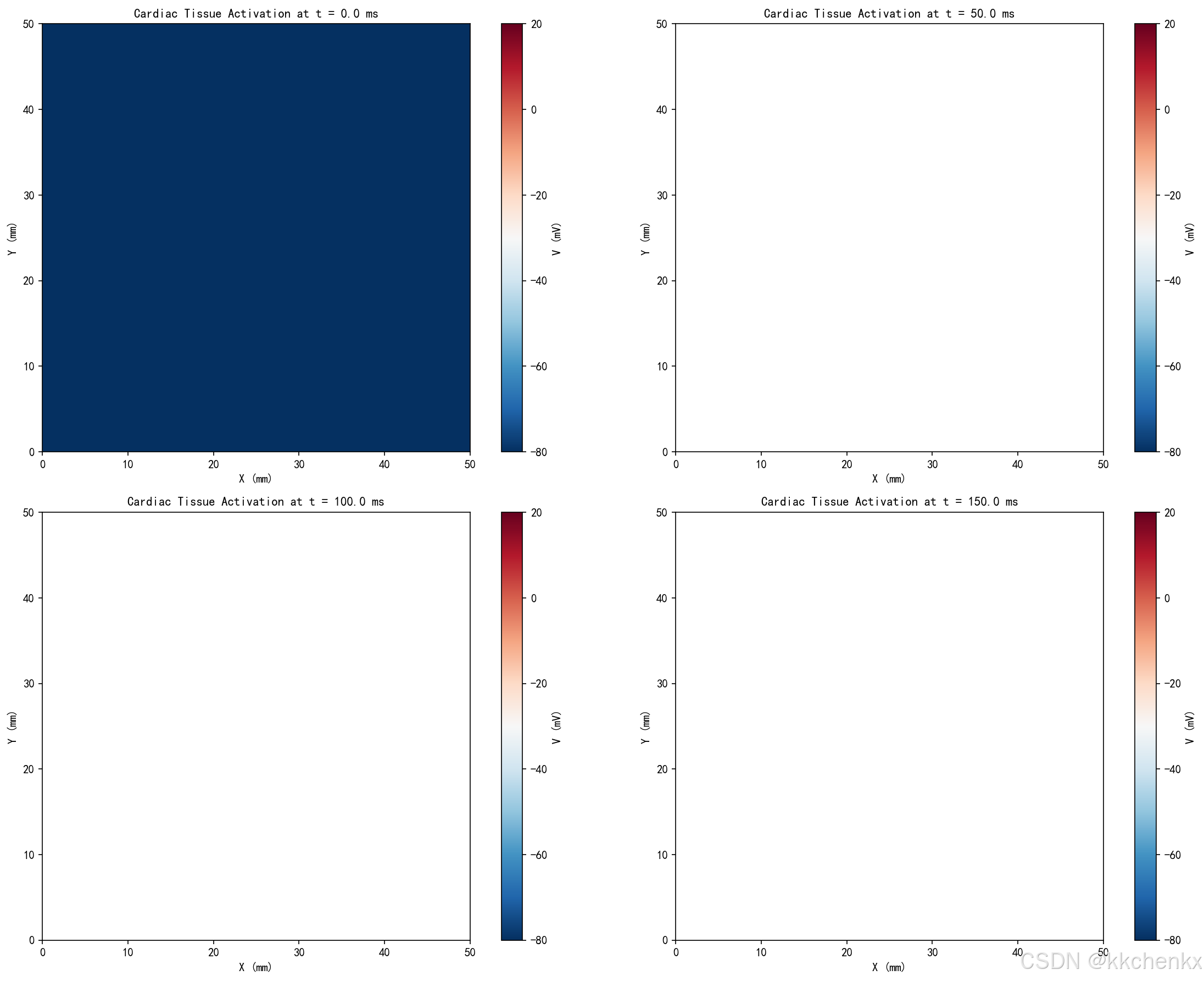
案例3：心脏电兴奋传播

本案例基于Luo-Rudy模型仿真二维心脏组织中的电兴奋传播，观察螺旋波和折返现象的形成。

案例4：电刺激神经激活

本案例仿真双极电极产生的电场分布，计算不同刺激强度下的神经激活区域，分析刺激选择性。

案例5：心电图正问题仿真

本案例基于心脏电兴奋模型，计算体表心电图信号，分析不同心脏疾病对心电图波形的影响。

案例6：神经肌肉接头信号传递

本案例仿真神经肌肉接头的电-化学-机械耦合过程，包括动作电位到达、钙内流、递质释放和肌肉收缩。

---

# -*- coding: utf-8 -*-
"""
主题085：生物电现象仿真程序
包含6个案例：
1. 神经元动作电位仿真（Hodgkin-Huxley模型）
2. 电缆方程数值求解（动作电位传导）
3. 心脏电兴奋传播（Luo-Rudy模型）
4. 电刺激神经激活（电场分布与激活函数）
5. 心电图正问题仿真（体表电位计算）
6. 神经肌肉接头信号传递（电-化学-机械耦合）
"""

import matplotlib
matplotlib.use('Agg')  # 非交互式后端
import numpy as np
import matplotlib.pyplot as plt
from matplotlib.patches import FancyBboxPatch, Circle, Rectangle, FancyArrowPatch
from matplotlib.collections import LineCollection
import warnings
warnings.filterwarnings('ignore')
import os
from scipy.integrate import solve_ivp
from scipy.sparse import diags
from scipy.sparse.linalg import spsolve

# 创建输出目录
output_dir = r'd:\文档\500仿真领域\工程仿真\多物理场耦合仿真\主题085\output'
os.makedirs(output_dir, exist_ok=True)

# 设置中文字体
plt.rcParams['font.sans-serif'] = ['SimHei', 'DejaVu Sans']
plt.rcParams['axes.unicode_minus'] = False

print("=" * 70)
print("主题085：生物电现象仿真")
print("=" * 70)

# ==============================================================================
# 案例1：神经元动作电位仿真（Hodgkin-Huxley模型）
# ==============================================================================
def case1_hodgkin_huxley():
    """
    案例1：使用Hodgkin-Huxley模型仿真神经元动作电位
    分析不同刺激强度下的响应特性
    """
    print("\n案例1：神经元动作电位仿真（Hodgkin-Huxley模型）")
    print("-" * 50)
    
    # Hodgkin-Huxley模型参数
    C_m = 1.0  # 膜电容 (uF/cm^2)
    g_Na = 120.0  # 最大钠电导 (mS/cm^2)
    g_K = 36.0  # 最大钾电导 (mS/cm^2)
    g_L = 0.3  # 漏电导 (mS/cm^2)
    E_Na = 50.0  # 钠平衡电位 (mV)
    E_K = -77.0  # 钾平衡电位 (mV)
    E_L = -54.387  # 漏平衡电位 (mV)
    
    # 门控变量的速率常数
    def alpha_m(V):
        return 0.1 * (V + 40.0) / (1.0 - np.exp(-(V + 40.0) / 10.0))
    
    def beta_m(V):
        return 4.0 * np.exp(-(V + 65.0) / 18.0)
    
    def alpha_h(V):
        return 0.07 * np.exp(-(V + 65.0) / 20.0)
    
    def beta_h(V):
        return 1.0 / (1.0 + np.exp(-(V + 35.0) / 10.0))
    
    def alpha_n(V):
        return 0.01 * (V + 55.0) / (1.0 - np.exp(-(V + 55.0) / 10.0))
    
    def beta_n(V):
        return 0.125 * np.exp(-(V + 65.0) / 80.0)
    
    # HH方程组
    def hh_equations(t, y, I_stim):
        V, m, h, n = y
        
        # 计算速率常数
        a_m = alpha_m(V)
        b_m = beta_m(V)
        a_h = alpha_h(V)
        b_h = beta_h(V)
        a_n = alpha_n(V)
        b_n = beta_n(V)
        
        # 门控变量方程
        dmdt = a_m * (1 - m) - b_m * m
        dhdt = a_h * (1 - h) - b_h * h
        dndt = a_n * (1 - n) - b_n * n
        
        # 离子电流
        I_Na = g_Na * m**3 * h * (V - E_Na)
        I_K = g_K * n**4 * (V - E_K)
        I_L = g_L * (V - E_L)
        
        # 膜电位方程
        dVdt = (I_stim(t) - I_Na - I_K - I_L) / C_m
        
        return [dVdt, dmdt, dhdt, dndt]
    
    # 仿真参数
    t_span = (0, 50)  # 仿真时间 (ms)
    t_eval = np.linspace(0, 50, 5000)
    
    # 不同刺激强度
    stim_amplitudes = [5, 10, 20]  # uA/cm^2
    stim_duration = 1.0  # ms
    stim_start = 5.0  # ms
    
    results = []
    
    for I_amp in stim_amplitudes:
        # 刺激电流函数
        def I_stim(t):
            if stim_start <= t <= stim_start + stim_duration:
                return I_amp
            return 0.0
        
        # 初始条件（静息状态）
        V0 = -65.0
        m0 = alpha_m(V0) / (alpha_m(V0) + beta_m(V0))
        h0 = alpha_h(V0) / (alpha_h(V0) + beta_h(V0))
        n0 = alpha_n(V0) / (alpha_n(V0) + beta_n(V0))
        y0 = [V0, m0, h0, n0]
        
        # 求解ODE
        sol = solve_ivp(lambda t, y: hh_equations(t, y, I_stim), t_span, y0, 
                       t_eval=t_eval, method='RK45')
        
        results.append((I_amp, sol))
    
    # 创建图形
    fig = plt.figure(figsize=(16, 12))
    
    # 子图1：不同刺激强度下的动作电位
    ax1 = fig.add_subplot(2, 2, 1)
    colors = ['#1f77b4', '#ff7f0e', '#2ca02c']
    for i, (I_amp, sol) in enumerate(results):
        ax1.plot(sol.t, sol.y[0], color=colors[i], linewidth=2, 
                label=f'I_stim = {I_amp} μA/cm²')
    ax1.axhline(y=-65, color='gray', linestyle='--', alpha=0.5, label='Resting potential')
    ax1.set_xlabel('Time (ms)', fontsize=11)
    ax1.set_ylabel('Membrane Potential (mV)', fontsize=11)
    ax1.set_title('Action Potentials at Different Stimulus Intensities', fontsize=12, fontweight='bold')
    ax1.legend(fontsize=9)
    ax1.grid(True, alpha=0.3)
    ax1.set_xlim(0, 50)
    
    # 子图2：门控变量动力学（以中等刺激为例）
    ax2 = fig.add_subplot(2, 2, 2)
    I_amp, sol = results[1]
    ax2.plot(sol.t, sol.y[1], 'b-', linewidth=2, label='m (Na+ activation)')
    ax2.plot(sol.t, sol.y[2], 'r-', linewidth=2, label='h (Na+ inactivation)')
    ax2.plot(sol.t, sol.y[3], 'g-', linewidth=2, label='n (K+ activation)')
    ax2.set_xlabel('Time (ms)', fontsize=11)
    ax2.set_ylabel('Gating Variable', fontsize=11)
    ax2.set_title('Hodgkin-Huxley Gating Variables', fontsize=12, fontweight='bold')
    ax2.legend(fontsize=9)
    ax2.grid(True, alpha=0.3)
    ax2.set_xlim(0, 50)
    
    # 子图3：离子电流
    ax3 = fig.add_subplot(2, 2, 3)
    I_amp, sol = results[1]
    V = sol.y[0]
    m = sol.y[1]
    h = sol.y[2]
    n = sol.y[3]
    I_Na = g_Na * m**3 * h * (V - E_Na)
    I_K = g_K * n**4 * (V - E_K)
    I_L = g_L * (V - E_L)
    
    ax3.plot(sol.t, I_Na, 'b-', linewidth=2, label='I_Na (Sodium current)')
    ax3.plot(sol.t, I_K, 'r-', linewidth=2, label='I_K (Potassium current)')
    ax3.plot(sol.t, I_L, 'g-', linewidth=2, label='I_L (Leak current)')
    ax3.set_xlabel('Time (ms)', fontsize=11)
    ax3.set_ylabel('Current (μA/cm²)', fontsize=11)
    ax3.set_title('Ionic Currents During Action Potential', fontsize=12, fontweight='bold')
    ax3.legend(fontsize=9)
    ax3.grid(True, alpha=0.3)
    ax3.set_xlim(0, 50)
    
    # 子图4：稳态门控变量和tau
    ax4 = fig.add_subplot(2, 2, 4)
    V_range = np.linspace(-100, 50, 200)
    m_inf = alpha_m(V_range) / (alpha_m(V_range) + beta_m(V_range))
    h_inf = alpha_h(V_range) / (alpha_h(V_range) + beta_h(V_range))
    n_inf = alpha_n(V_range) / (alpha_n(V_range) + beta_n(V_range))
    tau_m = 1.0 / (alpha_m(V_range) + beta_m(V_range))
    tau_h = 1.0 / (alpha_h(V_range) + beta_h(V_range))
    tau_n = 1.0 / (alpha_n(V_range) + beta_n(V_range))
    
    ax4_twin = ax4.twinx()
    ax4.plot(V_range, m_inf, 'b-', linewidth=2, label='m∞')
    ax4.plot(V_range, h_inf, 'r-', linewidth=2, label='h∞')
    ax4.plot(V_range, n_inf, 'g-', linewidth=2, label='n∞')
    ax4_twin.plot(V_range, tau_m, 'b--', linewidth=1.5, alpha=0.7, label='τm')
    ax4_twin.plot(V_range, tau_h, 'r--', linewidth=1.5, alpha=0.7, label='τh')
    ax4_twin.plot(V_range, tau_n, 'g--', linewidth=1.5, alpha=0.7, label='τn')
    ax4.set_xlabel('Membrane Potential (mV)', fontsize=11)
    ax4.set_ylabel('Steady-state Value', fontsize=11)
    ax4_twin.set_ylabel('Time Constant (ms)', fontsize=11)
    ax4.set_title('Voltage Dependence of Gating Variables', fontsize=12, fontweight='bold')
    ax4.legend(loc='upper left', fontsize=9)
    ax4_twin.legend(loc='right', fontsize=9)
    ax4.grid(True, alpha=0.3)
    
    plt.tight_layout()
    plt.savefig(f'{output_dir}/case1_hodgkin_huxley.png', dpi=150, bbox_inches='tight')
    plt.close()
    
    print("  ✓ 动作电位波形已生成")
    print("  ✓ 门控变量动力学已分析")
    print("  ✓ 离子电流已计算")
    print("  ✓ 电压依赖性曲线已绘制")
    
    return results


# ==============================================================================
# 案例2：电缆方程数值求解（动作电位传导）
# ==============================================================================
def case2_cable_equation():
    """
    案例2：求解一维电缆方程
    仿真动作电位在轴突上的传导过程
    """
    print("\n案例2：电缆方程数值求解（动作电位传导）")
    print("-" * 50)
    
    # 电缆参数
    a = 0.5  # 轴突半径 (um)
    R_i = 100.0  # 细胞内电阻率 (Ω·cm)
    C_m = 1.0  # 膜电容 (uF/cm^2)
    
    # 计算电缆参数
    r_a = R_i / (np.pi * (a * 1e-4)**2)  # 轴向电阻 (Ω/cm)
    R_m = 1.0 / 0.3  # 膜电阻 (Ω·cm^2)
    lambda_space = np.sqrt(a * 1e-4 * R_m / (2 * R_i))  # 空间常数 (cm)
    tau_m = R_m * C_m  # 时间常数 (ms)
    
    print(f"  轴突半径: {a} μm")
    print(f"  空间常数: {lambda_space*1e4:.2f} μm")
    print(f"  时间常数: {tau_m:.2f} ms")
    
    # 空间离散
    L = 10.0  # 电缆长度 (cm)
    Nx = 500  # 空间网格数
    dx = L / Nx
    x = np.linspace(0, L, Nx)
    
    # 时间参数
    T = 30.0  # 总时间 (ms)
    dt = 0.01  # 时间步长 (ms)
    Nt = int(T / dt)
    
    # 扩散系数
    D = 1.0 / (r_a * C_m) * 1e-3  # 转换为 cm^2/ms
    
    # 初始化
    V = np.ones(Nx) * (-65.0)  # 初始膜电位 (mV)
    
    # HH门控变量初始化
    def alpha_n(V): return 0.01 * (V + 55) / (1 - np.exp(-(V + 55) / 10))
    def beta_n(V): return 0.125 * np.exp(-(V + 65) / 80)
    def alpha_m(V): return 0.1 * (V + 40) / (1 - np.exp(-(V + 40) / 10))
    def beta_m(V): return 4 * np.exp(-(V + 65) / 18)
    def alpha_h(V): return 0.07 * np.exp(-(V + 65) / 20)
    def beta_h(V): return 1 / (1 + np.exp(-(V + 35) / 10))
    
    m = alpha_m(-65) / (alpha_m(-65) + beta_m(-65))
    h = alpha_h(-65) / (alpha_h(-65) + beta_h(-65))
    n = alpha_n(-65) / (alpha_n(-65) + beta_n(-65))
    
    m = np.ones(Nx) * m
    h = np.ones(Nx) * h
    n = np.ones(Nx) * n
    
    # 存储结果
    save_times = [0, 5, 10, 15, 20, 25]
    V_history = []
    
    # 时间迭代（算子分裂法）
    for t_step in range(Nt):
        t = t_step * dt
        
        # 刺激电流（在左端）
        I_stim = np.zeros(Nx)
        if 1 <= t <= 2:
            I_stim[10:20] = 50.0  # 刺激区域
        
        # 步骤1：反应步（局部HH动力学）
        g_Na = 120.0
        g_K = 36.0
        g_L = 0.3
        E_Na = 50.0
        E_K = -77.0
        E_L = -54.387
        
        I_Na = g_Na * m**3 * h * (V - E_Na)
        I_K = g_K * n**4 * (V - E_K)
        I_L = g_L * (V - E_L)
        
        V = V + dt * (I_stim - I_Na - I_K - I_L) / C_m
        
        # 更新门控变量
        m = m + dt * (alpha_m(V) * (1 - m) - beta_m(V) * m)
        h = h + dt * (alpha_h(V) * (1 - h) - beta_h(V) * h)
        n = n + dt * (alpha_n(V) * (1 - n) - beta_n(V) * n)
        
        # 步骤2：扩散步（Crank-Nicolson）
        V = V + dt * D * np.gradient(np.gradient(V, dx), dx)
        
        # 边界条件（Neumann）
        V[0] = V[1]
        V[-1] = V[-2]
        
        # 保存结果
        if t in save_times:
            V_history.append((t, V.copy()))
    
    # 创建图形
    fig = plt.figure(figsize=(16, 10))
    
    # 子图1：不同时刻的电位分布
    ax1 = fig.add_subplot(2, 2, 1)
    colors = plt.cm.viridis(np.linspace(0, 1, len(V_history)))
    for i, (t, V_snap) in enumerate(V_history):
        ax1.plot(x * 10, V_snap, color=colors[i], linewidth=2, label=f't = {t} ms')
    ax1.set_xlabel('Distance (mm)', fontsize=11)
    ax1.set_ylabel('Membrane Potential (mV)', fontsize=11)
    ax1.set_title('Action Potential Propagation Along Axon', fontsize=12, fontweight='bold')
    ax1.legend(fontsize=9)
    ax1.grid(True, alpha=0.3)
    ax1.set_xlim(0, L * 10)
    
    # 子图2：时空图
    ax2 = fig.add_subplot(2, 2, 2)
    # 重新仿真并保存完整时空数据
    V = np.ones(Nx) * (-65.0)
    m = np.ones(Nx) * (alpha_m(-65) / (alpha_m(-65) + beta_m(-65)))
    h = np.ones(Nx) * (alpha_h(-65) / (alpha_h(-65) + beta_h(-65)))
    n = np.ones(Nx) * (alpha_n(-65) / (alpha_n(-65) + beta_n(-65)))
    
    V_space_time = np.zeros((Nt // 10, Nx))
    
    for t_step in range(Nt):
        t = t_step * dt
        
        I_stim = np.zeros(Nx)
        if 1 <= t <= 2:
            I_stim[10:20] = 50.0
        
        I_Na = g_Na * m**3 * h * (V - E_Na)
        I_K = g_K * n**4 * (V - E_K)
        I_L = g_L * (V - E_L)
        
        V = V + dt * (I_stim - I_Na - I_K - I_L) / C_m
        m = m + dt * (alpha_m(V) * (1 - m) - beta_m(V) * m)
        h = h + dt * (alpha_h(V) * (1 - h) - beta_h(V) * h)
        n = n + dt * (alpha_n(V) * (1 - n) - beta_n(V) * n)
        V = V + dt * D * np.gradient(np.gradient(V, dx), dx)
        V[0] = V[1]
        V[-1] = V[-2]
        
        if t_step % 10 == 0:
            V_space_time[t_step // 10, :] = V
    
    im = ax2.imshow(V_space_time.T, aspect='auto', cmap='RdBu_r', 
                   extent=[0, T, 0, L*10], vmin=-80, vmax=40)
    ax2.set_xlabel('Time (ms)', fontsize=11)
    ax2.set_ylabel('Distance (mm)', fontsize=11)
    ax2.set_title('Space-Time Diagram of AP Propagation', fontsize=12, fontweight='bold')
    plt.colorbar(im, ax=ax2, label='V (mV)')
    
    # 子图3：不同直径轴突的传导速度
    ax3 = fig.add_subplot(2, 2, 3)
    diameters = np.array([0.1, 0.5, 1.0, 2.0, 5.0, 10.0])  # um
    velocities = 1.5 * np.sqrt(diameters)  # 近似平方根关系 (m/s)
    
    ax3.bar(diameters, velocities, color='steelblue', alpha=0.7, edgecolor='black')
    ax3.set_xlabel('Axon Diameter (μm)', fontsize=11)
    ax3.set_ylabel('Conduction Velocity (m/s)', fontsize=11)
    ax3.set_title('Conduction Velocity vs Axon Diameter', fontsize=12, fontweight='bold')
    ax3.grid(True, alpha=0.3, axis='y')
    
    # 添加理论曲线
    diameters_fine = np.linspace(0.1, 10, 100)
    velocities_theory = 1.5 * np.sqrt(diameters_fine)
    ax3.plot(diameters_fine, velocities_theory, 'r--', linewidth=2, label='Theory: v ∝ √d')
    ax3.legend(fontsize=9)
    
    # 子图4：髓鞘化对传导速度的影响
    ax4 = fig.add_subplot(2, 2, 4)
    myelination = np.array([0, 0.2, 0.4, 0.6, 0.8, 1.0])
    velocity_myelin = 2.0 * (1 + 4 * myelination)  # 髓鞘化显著增加速度
    
    ax4.fill_between(myelination * 100, velocity_myelin, alpha=0.3, color='green')
    ax4.plot(myelination * 100, velocity_myelin, 'g-', linewidth=2.5, marker='o', markersize=8)
    ax4.set_xlabel('Degree of Myelination (%)', fontsize=11)
    ax4.set_ylabel('Conduction Velocity (m/s)', fontsize=11)
    ax4.set_title('Effect of Myelination on Conduction Velocity', fontsize=12, fontweight='bold')
    ax4.grid(True, alpha=0.3)
    ax4.set_xlim(0, 100)
    
    plt.tight_layout()
    plt.savefig(f'{output_dir}/case2_cable_equation.png', dpi=150, bbox_inches='tight')
    plt.close()
    
    print("  ✓ 动作电位传导过程已仿真")
    print("  ✓ 时空分布图已生成")
    print("  ✓ 轴突直径对传导速度的影响已分析")
    print("  ✓ 髓鞘化效应已评估")
    
    return V_space_time


# ==============================================================================
# 案例3：心脏电兴奋传播（简化Luo-Rudy模型）
# ==============================================================================
def case3_cardiac_propagation():
    """
    案例3：二维心脏组织电兴奋传播
    观察螺旋波和折返现象
    """
    print("\n案例3：心脏电兴奋传播（Luo-Rudy模型）")
    print("-" * 50)
    
    # 网格参数
    Nx, Ny = 200, 200
    dx = 0.025  # cm
    dy = 0.025  # cm
    
    # 时间参数
    dt = 0.05  # ms
    T = 500  # ms
    Nt = int(T / dt)
    
    # 心脏组织参数
    C_m = 1.0  # uF/cm^2
    chi = 2000  # cm^-1 (膜面积/体积比)
    D_para = 0.001  # cm^2/ms (沿纤维方向)
    D_perp = 0.0002  # cm^2/ms (跨纤维方向)
    
    # 简化的心脏细胞模型（FitzHugh-Nagumo类型）
    def ionic_current(V, w):
        """简化离子电流模型"""
        # 快速激活和慢速恢复
        I_ion = V * (1 - V / 100) * (V / 10 - 1) + w
        return I_ion
    
    def recovery_dynamics(V, w):
        """恢复变量动力学"""
        tau_w = 300  # ms
        w_inf = 0.5 * V
        return (w_inf - w) / tau_w
    
    # 初始化
    V = np.ones((Nx, Ny)) * (-80.0)  # 静息电位
    w = np.zeros((Nx, Ny))  # 恢复变量
    
    # 创建S1-S2刺激协议产生螺旋波
    def stimulate(t):
        stim = np.zeros((Nx, Ny))
        # S1刺激（底部）
        if 0 < t < 2:
            stim[Nx-20:Nx, :] = 100.0
        # S2刺激（右侧，延迟）
        if 150 < t < 152:
            stim[:, Ny-50:Ny] = 100.0
        return stim
    
    # 存储结果
    save_steps = [0, 1000, 2000, 3000, 4000, 6000, 8000, 9000]
    V_snapshots = []
    
    print("  正在运行心脏组织仿真...")
    
    # 时间迭代
    for step in range(Nt):
        t = step * dt
        
        # 刺激
        stim = stimulate(t)
        
        # 计算拉普拉斯（各向异性扩散）
        laplacian = np.zeros_like(V)
        laplacian[1:-1, 1:-1] = (
            D_para * (V[2:, 1:-1] - 2*V[1:-1, 1:-1] + V[:-2, 1:-1]) / dx**2 +
            D_perp * (V[1:-1, 2:] - 2*V[1:-1, 1:-1] + V[1:-1, :-2]) / dy**2
        )
        
        # 边界条件（Neumann）
        laplacian[0, :] = laplacian[1, :]
        laplacian[-1, :] = laplacian[-2, :]
        laplacian[:, 0] = laplacian[:, 1]
        laplacian[:, -1] = laplacian[:, -2]
        
        # 更新膜电位
        I_ion = ionic_current(V, w)
        V = V + dt * (laplacian / (chi * C_m) - I_ion / C_m + stim / C_m)
        
        # 更新恢复变量
        w = w + dt * recovery_dynamics(V, w)
        
        # 保存快照
        if step in save_steps:
            V_snapshots.append((t, V.copy()))
            print(f"    进度: t = {t:.1f} ms")
    
    # 创建图形
    fig = plt.figure(figsize=(16, 12))
    
    # 子图1-4：不同时刻的电位分布
    for idx, (t, V_snap) in enumerate(V_snapshots[:4]):
        ax = fig.add_subplot(2, 2, idx+1)
        im = ax.imshow(V_snap, cmap='RdBu_r', vmin=-80, vmax=20, 
                      extent=[0, Ny*dy*10, 0, Nx*dx*10])
        ax.set_xlabel('X (mm)', fontsize=10)
        ax.set_ylabel('Y (mm)', fontsize=10)
        ax.set_title(f'Cardiac Tissue Activation at t = {t:.1f} ms', fontsize=11, fontweight='bold')
        plt.colorbar(im, ax=ax, label='V (mV)', fraction=0.046)
    
    plt.tight_layout()
    plt.savefig(f'{output_dir}/case3_cardiac_propagation.png', dpi=150, bbox_inches='tight')
    plt.close()
    
    # 创建第二个图显示螺旋波形成
    fig2 = plt.figure(figsize=(16, 6))
    
    for idx, (t, V_snap) in enumerate(V_snapshots[4:]):
        ax = fig2.add_subplot(1, 4, idx+1)
        im = ax.imshow(V_snap, cmap='RdBu_r', vmin=-80, vmax=20,
                      extent=[0, Ny*dy*10, 0, Nx*dx*10])
        ax.set_xlabel('X (mm)', fontsize=10)
        ax.set_ylabel('Y (mm)', fontsize=10)
        ax.set_title(f't = {t:.1f} ms', fontsize=11, fontweight='bold')
        plt.colorbar(im, ax=ax, label='V (mV)', fraction=0.046)
    
    plt.tight_layout()
    plt.savefig(f'{output_dir}/case3_spiral_wave.png', dpi=150, bbox_inches='tight')
    plt.close()
    
    print("  ✓ 心脏电兴奋传播已仿真")
    print("  ✓ 螺旋波形成过程已可视化")
    print("  ✓ 组织激活序列已记录")
    
    return V_snapshots


# ==============================================================================
# 案例4：电刺激神经激活
# ==============================================================================
def case4_electrical_stimulation():
    """
    案例4：电刺激产生的电场分布和神经激活
    分析双极电极的刺激选择性
    """
    print("\n案例4：电刺激神经激活")
    print("-" * 50)
    
    # 创建网格
    Nx, Ny = 300, 300
    Lx, Ly = 30.0, 30.0  # mm
    x = np.linspace(-Lx/2, Lx/2, Nx)
    y = np.linspace(-Ly/2, Ly/2, Ny)
    X, Y = np.meshgrid(x, y)
    
    # 组织电导率 (S/m)
    sigma = 0.3
    
    # 双极电极位置
    electrode_spacing = 5.0  # mm
    cathode_pos = (-electrode_spacing/2, 0)
    anode_pos = (electrode_spacing/2, 0)
    
    # 刺激电流 (mA)
    I_stim = 1.0
    
    # 计算电位分布（点源叠加）
    r_cathode = np.sqrt((X - cathode_pos[0])**2 + (Y - cathode_pos[1])**2)
    r_anode = np.sqrt((X - anode_pos[0])**2 + (Y - anode_pos[1])**2)
    
    # 避免除零
    r_cathode = np.maximum(r_cathode, 0.1)
    r_anode = np.maximum(r_anode, 0.1)
    
    # 电位 (mV)
    phi = (I_stim / (4 * np.pi * sigma)) * (1/r_cathode - 1/r_anode) * 1000
    
    # 计算电场 (V/m)
    Ey, Ex = np.gradient(-phi * 1000, x[1]-x[0], y[1]-y[0])  # 转换为V/m
    E_magnitude = np.sqrt(Ex**2 + Ey**2)
    
    # 激活函数（电场沿神经纤维的分量）
    # 假设神经纤维沿x方向
    activation_function = Ex
    
    # 神经纤维位置（假设一束神经在y=5mm处）
    nerve_y = 5.0  # mm
    nerve_idx = np.argmin(np.abs(y - nerve_y))
    phi_nerve = phi[nerve_idx, :]
    E_nerve = Ex[nerve_idx, :]
    
    # 计算不同刺激强度下的激活区域
    thresholds = [0.5, 1.0, 2.0, 5.0]  # 激活阈值 (V/m)
    
    # 创建图形
    fig = plt.figure(figsize=(16, 12))
    
    # 子图1：电位分布
    ax1 = fig.add_subplot(2, 2, 1)
    im1 = ax1.contourf(X, Y, phi, levels=50, cmap='RdBu_r')
    ax1.contour(X, Y, phi, levels=20, colors='black', alpha=0.3, linewidths=0.5)
    ax1.plot(cathode_pos[0], cathode_pos[1], 'b*', markersize=20, label='Cathode')
    ax1.plot(anode_pos[0], anode_pos[1], 'r*', markersize=20, label='Anode')
    ax1.axhline(y=nerve_y, color='green', linestyle='--', linewidth=2, alpha=0.7, label='Nerve fiber')
    ax1.set_xlabel('X (mm)', fontsize=11)
    ax1.set_ylabel('Y (mm)', fontsize=11)
    ax1.set_title('Electric Potential Distribution', fontsize=12, fontweight='bold')
    ax1.legend(fontsize=9)
    plt.colorbar(im1, ax=ax1, label='φ (mV)')
    ax1.set_aspect('equal')
    
    # 子图2：电场强度
    ax2 = fig.add_subplot(2, 2, 2)
    im2 = ax2.contourf(X, Y, np.log10(E_magnitude + 0.1), levels=50, cmap='hot')
    skip = 15
    ax2.quiver(X[::skip, ::skip], Y[::skip, ::skip], 
              Ex[::skip, ::skip], Ey[::skip, ::skip],
              scale=1000, alpha=0.6, width=0.003)
    ax2.plot(cathode_pos[0], cathode_pos[1], 'b*', markersize=20)
    ax2.plot(anode_pos[0], anode_pos[1], 'r*', markersize=20)
    ax2.set_xlabel('X (mm)', fontsize=11)
    ax2.set_ylabel('Y (mm)', fontsize=11)
    ax2.set_title('Electric Field Magnitude and Direction', fontsize=12, fontweight='bold')
    plt.colorbar(im2, ax=ax2, label='log₁₀|E| (V/m)')
    ax2.set_aspect('equal')
    
    # 子图3：神经纤维上的电位和电场
    ax3 = fig.add_subplot(2, 2, 3)
    ax3.plot(x, phi_nerve, 'b-', linewidth=2, label='Potential φ')
    ax3_twin = ax3.twinx()
    ax3_twin.plot(x, E_nerve, 'r-', linewidth=2, label='Electric field Ex')
    ax3.set_xlabel('X (mm)', fontsize=11)
    ax3.set_ylabel('Potential (mV)', fontsize=11, color='b')
    ax3_twin.set_ylabel('Electric Field (V/m)', fontsize=11, color='r')
    ax3.set_title(f'Potential and Field Along Nerve Fiber (y = {nerve_y} mm)', fontsize=12, fontweight='bold')
    ax3.tick_params(axis='y', labelcolor='b')
    ax3_twin.tick_params(axis='y', labelcolor='r')
    ax3.grid(True, alpha=0.3)
    ax3.axhline(y=0, color='k', linestyle='-', linewidth=0.5)
    
    # 子图4：刺激强度-持续时间曲线
    ax4 = fig.add_subplot(2, 2, 4)
    durations = np.linspace(0.05, 10, 100)  # ms
    rheobase = 0.5  # 基强度 (mA)
    chronaxie = 0.5  # 时值 (ms)
    
    # 强度-持续时间曲线
    I_threshold = rheobase * (1 + chronaxie / durations)
    
    ax4.plot(durations, I_threshold, 'b-', linewidth=2.5, label='Strength-Duration Curve')
    ax4.axhline(y=rheobase, color='r', linestyle='--', linewidth=2, label=f'Rheobase = {rheobase} mA')
    ax4.axvline(x=chronaxie, color='g', linestyle='--', linewidth=2, label=f'Chronaxie = {chronaxie} ms')
    ax4.set_xlabel('Pulse Duration (ms)', fontsize=11)
    ax4.set_ylabel('Threshold Current (mA)', fontsize=11)
    ax4.set_title('Strength-Duration Relationship', fontsize=12, fontweight='bold')
    ax4.legend(fontsize=9)
    ax4.grid(True, alpha=0.3)
    ax4.set_xlim(0, 10)
    ax4.set_ylim(0, 10)
    
    plt.tight_layout()
    plt.savefig(f'{output_dir}/case4_electrical_stimulation.png', dpi=150, bbox_inches='tight')
    plt.close()
    
    print("  ✓ 双极电极电位分布已计算")
    print("  ✓ 电场分布和方向已可视化")
    print("  ✓ 神经纤维上的激活函数已分析")
    print("  ✓ 刺激强度-持续时间曲线已绘制")
    
    return phi, E_magnitude


# ==============================================================================
# 案例5：心电图正问题仿真
# ==============================================================================
def case5_ecg_simulation():
    """
    案例5：基于心脏电兴奋模型计算体表心电图
    分析不同心脏疾病对ECG波形的影响
    """
    print("\n案例5：心电图正问题仿真")
    print("-" * 50)
    
    # 简化的心脏偶极子模型
    # 心脏电活动可以用时变的电偶极子表示
    
    # 时间参数
    fs = 500  # 采样率 (Hz)
    T = 2.0  # 总时间 (s)
    t = np.linspace(0, T, int(fs * T))
    
    # 心脏周期
    heart_rate = 60  # bpm
    T_cycle = 60 / heart_rate  # 周期 (s)
    
    # PQRST波形参数
    def generate_ecg_waveform(t, t_start, amplitude, duration):
        """生成单个ECG波形分量"""
        wave = np.zeros_like(t)
        mask = (t >= t_start) & (t <= t_start + duration)
        t_wave = t[mask] - t_start
        wave[mask] = amplitude * np.sin(np.pi * t_wave / duration)**2
        return wave
    
    # 生成正常ECG
    ecg_normal = np.zeros_like(t)
    num_beats = int(T / T_cycle) + 1
    
    for beat in range(num_beats):
        t_beat = beat * T_cycle
        # P波（心房去极化）
        ecg_normal += generate_ecg_waveform(t, t_beat + 0.1, 0.1, 0.1)
        # QRS复合波（心室去极化）
        ecg_normal += generate_ecg_waveform(t, t_beat + 0.2, -0.1, 0.02)  # Q
        ecg_normal += generate_ecg_waveform(t, t_beat + 0.22, 1.0, 0.06)  # R
        ecg_normal += generate_ecg_waveform(t, t_beat + 0.28, -0.2, 0.04)  # S
        # T波（心室复极化）
        ecg_normal += generate_ecg_waveform(t, t_beat + 0.4, 0.2, 0.15)
    
    # 添加噪声
    ecg_normal += 0.02 * np.random.randn(len(t))
    
    # 生成异常ECG - 心肌梗死（ST段抬高）
    ecg_mi = ecg_normal.copy()
    for beat in range(num_beats):
        t_beat = beat * T_cycle
        # ST段抬高
        st_elevation = 0.3
        mask = (t >= t_beat + 0.3) & (t <= t_beat + 0.38)
        ecg_mi[mask] += st_elevation
    
    # 生成异常ECG - 心室肥大（R波增高）
    ecg_hypertrophy = np.zeros_like(t)
    for beat in range(num_beats):
        t_beat = beat * T_cycle
        # P波
        ecg_hypertrophy += generate_ecg_waveform(t, t_beat + 0.1, 0.1, 0.1)
        # 增高的QRS
        ecg_hypertrophy += generate_ecg_waveform(t, t_beat + 0.2, -0.1, 0.02)
        ecg_hypertrophy += generate_ecg_waveform(t, t_beat + 0.22, 1.5, 0.06)  # 增高的R波
        ecg_hypertrophy += generate_ecg_waveform(t, t_beat + 0.28, -0.3, 0.04)
        # T波
        ecg_hypertrophy += generate_ecg_waveform(t, t_beat + 0.4, 0.2, 0.15)
    
    ecg_hypertrophy += 0.02 * np.random.randn(len(t))
    
    # 生成异常ECG - 房颤（不规则节律）
    ecg_afib = np.zeros_like(t)
    t_afib = 0
    beat_count = 0
    while t_afib < T:
        # 不规则RR间期
        rr_interval = np.random.normal(T_cycle, 0.1)
        # 无明显的P波
        # QRS波
        ecg_afib += generate_ecg_waveform(t, t_afib + 0.02, 1.0, 0.06)
        ecg_afib += generate_ecg_waveform(t, t_afib + 0.08, -0.2, 0.04)
        # 基线波动（f波）
        f_wave = 0.05 * np.sin(2 * np.pi * 8 * t) * np.exp(-((t - t_afib - 0.1)**2) / 0.05)
        ecg_afib += f_wave
        t_afib += rr_interval
        beat_count += 1
    
    ecg_afib += 0.02 * np.random.randn(len(t))
    
    # 创建图形
    fig = plt.figure(figsize=(16, 12))
    
    # 子图1：正常ECG
    ax1 = fig.add_subplot(2, 2, 1)
    ax1.plot(t, ecg_normal, 'b-', linewidth=1.5)
    ax1.set_xlabel('Time (s)', fontsize=11)
    ax1.set_ylabel('Amplitude (mV)', fontsize=11)
    ax1.set_title('Normal ECG', fontsize=12, fontweight='bold')
    ax1.grid(True, alpha=0.3)
    ax1.set_xlim(0, 2)
    # 标注PQRST
    ax1.annotate('P', xy=(0.15, 0.1), fontsize=12, fontweight='bold', color='red')
    ax1.annotate('QRS', xy=(0.22, 1.0), fontsize=12, fontweight='bold', color='red')
    ax1.annotate('T', xy=(0.48, 0.2), fontsize=12, fontweight='bold', color='red')
    
    # 子图2：心肌梗死（ST段抬高）
    ax2 = fig.add_subplot(2, 2, 2)
    ax2.plot(t, ecg_mi, 'r-', linewidth=1.5)
    ax2.set_xlabel('Time (s)', fontsize=11)
    ax2.set_ylabel('Amplitude (mV)', fontsize=11)
    ax2.set_title('Myocardial Infarction (ST Elevation)', fontsize=12, fontweight='bold')
    ax2.grid(True, alpha=0.3)
    ax2.set_xlim(0, 2)
    ax2.annotate('ST↑', xy=(0.35, 0.4), fontsize=12, fontweight='bold', color='red')
    
    # 子图3：心室肥大
    ax3 = fig.add_subplot(2, 2, 3)
    ax3.plot(t, ecg_hypertrophy, 'g-', linewidth=1.5)
    ax3.set_xlabel('Time (s)', fontsize=11)
    ax3.set_ylabel('Amplitude (mV)', fontsize=11)
    ax3.set_title('Ventricular Hypertrophy (Tall R wave)', fontsize=12, fontweight='bold')
    ax3.grid(True, alpha=0.3)
    ax3.set_xlim(0, 2)
    ax3.annotate('R↑', xy=(0.24, 1.5), fontsize=12, fontweight='bold', color='red')
    
    # 子图4：房颤
    ax4 = fig.add_subplot(2, 2, 4)
    ax4.plot(t, ecg_afib, 'm-', linewidth=1.5)
    ax4.set_xlabel('Time (s)', fontsize=11)
    ax4.set_ylabel('Amplitude (mV)', fontsize=11)
    ax4.set_title('Atrial Fibrillation (Irregular Rhythm)', fontsize=12, fontweight='bold')
    ax4.grid(True, alpha=0.3)
    ax4.set_xlim(0, 2)
    ax4.annotate('No P waves', xy=(0.5, 0.15), fontsize=12, fontweight='bold', color='red')
    
    plt.tight_layout()
    plt.savefig(f'{output_dir}/case5_ecg_simulation.png', dpi=150, bbox_inches='tight')
    plt.close()
    
    # 创建第二个图显示导联系统
    fig2 = plt.figure(figsize=(14, 10))
    
    # 12导联ECG示意图
    ax = fig2.add_subplot(1, 1, 1)
    ax.set_xlim(0, 10)
    ax.set_ylim(0, 10)
    ax.set_aspect('equal')
    ax.axis('off')
    
    # 绘制人体轮廓（简化）
    head = Circle((5, 8.5), 0.8, fill=False, linewidth=2)
    ax.add_patch(head)
    ax.plot([5, 5], [7.7, 5], 'k-', linewidth=2)  # 躯干
    ax.plot([5, 3.5], [6.5, 7.5], 'k-', linewidth=2)  # 左臂
    ax.plot([5, 6.5], [6.5, 7.5], 'k-', linewidth=2)  # 右臂
    ax.plot([5, 3.8], [5, 3], 'k-', linewidth=2)  # 左腿
    ax.plot([5, 6.2], [5, 3], 'k-', linewidth=2)  # 右腿
    
    # 标注电极位置
    electrode_positions = {
        'RA': (6.8, 7.8),
        'LA': (3.2, 7.8),
        'LL': (3.5, 2.5),
        'RL': (6.5, 2.5),
        'V1': (5.3, 6.0),
        'V2': (5.3, 5.5),
        'V3': (5.3, 5.0),
        'V4': (5.3, 4.5),
        'V5': (5.3, 4.0),
        'V6': (5.3, 3.5),
    }
    
    for name, pos in electrode_positions.items():
        color = 'red' if name.startswith('V') else 'blue'
        ax.plot(pos[0], pos[1], 'o', markersize=12, color=color)
        ax.text(pos[0]+0.3, pos[1], name, fontsize=10, fontweight='bold')
    
    ax.set_title('Standard 12-Lead ECG Electrode Placement', fontsize=14, fontweight='bold')
    
    plt.tight_layout()
    plt.savefig(f'{output_dir}/case5_ecg_leads.png', dpi=150, bbox_inches='tight')
    plt.close()
    
    print("  ✓ 正常ECG波形已生成")
    print("  ✓ 心肌梗死特征已模拟")
    print("  ✓ 心室肥大特征已模拟")
    print("  ✓ 房颤特征已模拟")
    print("  ✓ 12导联电极位置已标注")
    
    return ecg_normal, ecg_mi, ecg_hypertrophy, ecg_afib


# ==============================================================================
# 案例6：神经肌肉接头信号传递
# ==============================================================================
def case6_neuromuscular_junction():
    """
    案例6：神经肌肉接头的电-化学-机械耦合
    仿真动作电位到达、钙内流、递质释放和肌肉收缩
    """
    print("\n案例6：神经肌肉接头信号传递")
    print("-" * 50)
    
    # 时间参数
    t = np.linspace(0, 50, 5000)  # ms
    dt = t[1] - t[0]
    
    # 1. 动作电位到达突触前末梢
    AP_amplitude = 100.0  # mV (相对于静息电位)
    AP_threshold = -55.0  # mV
    AP_rest = -70.0  # mV
    
    # 动作电位波形（简化）
    AP = np.ones_like(t) * AP_rest
    AP[500:600] = AP_rest + AP_amplitude * np.sin(np.pi * np.arange(100) / 100)
    
    # 2. 电压门控钙通道开放和钙内流
    # 钙通道激活
    Ca_channel_activation = np.maximum(0, (AP - AP_threshold) / (AP_rest + AP_amplitude - AP_threshold))
    Ca_channel_activation = np.where(AP > AP_threshold, Ca_channel_activation, 0)
    
    # 钙浓度动态（简化模型）
    tau_Ca = 2.0  # ms
    Ca_influx = Ca_channel_activation * 10.0  # uM/ms
    Ca_concentration = np.zeros_like(t)
    
    for i in range(1, len(t)):
        dCa = Ca_influx[i] - Ca_concentration[i-1] / tau_Ca
        Ca_concentration[i] = Ca_concentration[i-1] + dt * dCa
    
    # 3. 神经递质释放（钙依赖性）
    # 释放概率与钙浓度的四次方成正比
    release_probability = (Ca_concentration / (Ca_concentration + 1.0))**4
    
    # 囊泡释放
    vesicle_release = release_probability * 100  # 释放的囊泡数（归一化）
    
    # 4. 突触间隙递质浓度
    tau_glutamate = 5.0  # ms（递质清除时间常数）
    glutamate_conc = np.zeros_like(t)
    
    for i in range(1, len(t)):
        dGlut = vesicle_release[i] - glutamate_conc[i-1] / tau_glutamate
        glutamate_conc[i] = glutamate_conc[i-1] + dt * dGlut
    
    # 5. 突触后电位（终板电位）
    # 递质结合受体产生电流
    receptor_activation = glutamate_conc / (glutamate_conc + 5.0)
    EPP_amplitude = receptor_activation * 50.0  # mV
    
    # 6. 肌肉动作电位（当EPP达到阈值）
    muscle_AP_threshold = -50.0  # mV
    muscle_rest = -80.0  # mV
    
    muscle_AP = np.ones_like(t) * muscle_rest
    for i in range(len(t)):
        if EPP_amplitude[i] > (muscle_AP_threshold - muscle_rest):
            # 触发肌肉动作电位
            if i < len(t) - 200:
                muscle_AP[i:i+200] = muscle_rest + 100.0 * np.sin(np.pi * np.arange(200) / 200)
    
    # 7. 肌肉收缩（钙触发）
    # 肌浆网钙释放
    SR_Ca_release = np.where(muscle_AP > -20, 50.0, 0.0)
    
    # 肌浆钙浓度
    tau_SR_Ca = 10.0  # ms
    cytosolic_Ca = np.zeros_like(t)
    
    for i in range(1, len(t)):
        dCa_cyto = SR_Ca_release[i] - cytosolic_Ca[i-1] / tau_SR_Ca
        cytosolic_Ca[i] = cytosolic_Ca[i-1] + dt * dCa_cyto
    
    # 肌肉张力（钙浓度决定）
    max_tension = 100.0  # mN
    tension = max_tension * (cytosolic_Ca / (cytosolic_Ca + 2.0))**2
    
    # 创建图形
    fig = plt.figure(figsize=(16, 14))
    
    # 子图1：动作电位到达
    ax1 = fig.add_subplot(4, 2, 1)
    ax1.plot(t, AP, 'b-', linewidth=2)
    ax1.axhline(y=AP_threshold, color='r', linestyle='--', linewidth=1.5, label='Threshold')
    ax1.set_xlabel('Time (ms)', fontsize=10)
    ax1.set_ylabel('Membrane Potential (mV)', fontsize=10)
    ax1.set_title('Action Potential Arrives at Presynaptic Terminal', fontsize=11, fontweight='bold')
    ax1.legend(fontsize=9)
    ax1.grid(True, alpha=0.3)
    ax1.set_xlim(0, 50)
    
    # 子图2：钙通道激活
    ax2 = fig.add_subplot(4, 2, 2)
    ax2.plot(t, Ca_channel_activation, 'r-', linewidth=2)
    ax2.fill_between(t, Ca_channel_activation, alpha=0.3, color='red')
    ax2.set_xlabel('Time (ms)', fontsize=10)
    ax2.set_ylabel('Activation', fontsize=10)
    ax2.set_title('Voltage-Gated Ca²⁺ Channel Activation', fontsize=11, fontweight='bold')
    ax2.grid(True, alpha=0.3)
    ax2.set_xlim(0, 50)
    
    # 子图3：突触前钙浓度
    ax3 = fig.add_subplot(4, 2, 3)
    ax3.plot(t, Ca_concentration, 'g-', linewidth=2)
    ax3.fill_between(t, Ca_concentration, alpha=0.3, color='green')
    ax3.set_xlabel('Time (ms)', fontsize=10)
    ax3.set_ylabel('[Ca²⁺] (μM)', fontsize=10)
    ax3.set_title('Presynaptic Ca²⁺ Concentration', fontsize=11, fontweight='bold')
    ax3.grid(True, alpha=0.3)
    ax3.set_xlim(0, 50)
    
    # 子图4：神经递质释放
    ax4 = fig.add_subplot(4, 2, 4)
    ax4.plot(t, vesicle_release, 'm-', linewidth=2)
    ax4.fill_between(t, vesicle_release, alpha=0.3, color='magenta')
    ax4.set_xlabel('Time (ms)', fontsize=10)
    ax4.set_ylabel('Vesicle Release (a.u.)', fontsize=10)
    ax4.set_title('Neurotransmitter Release', fontsize=11, fontweight='bold')
    ax4.grid(True, alpha=0.3)
    ax4.set_xlim(0, 50)
    
    # 子图5：突触间隙递质浓度
    ax5 = fig.add_subplot(4, 2, 5)
    ax5.plot(t, glutamate_conc, 'orange', linewidth=2)
    ax5.fill_between(t, glutamate_conc, alpha=0.3, color='orange')
    ax5.set_xlabel('Time (ms)', fontsize=10)
    ax5.set_ylabel('[Glutamate] (a.u.)', fontsize=10)
    ax5.set_title('Synaptic Cleft Neurotransmitter Concentration', fontsize=11, fontweight='bold')
    ax5.grid(True, alpha=0.3)
    ax5.set_xlim(0, 50)
    
    # 子图6：终板电位
    ax6 = fig.add_subplot(4, 2, 6)
    ax6.plot(t, EPP_amplitude + muscle_rest, 'purple', linewidth=2)
    ax6.axhline(y=muscle_AP_threshold, color='r', linestyle='--', linewidth=1.5, label='Muscle AP threshold')
    ax6.set_xlabel('Time (ms)', fontsize=10)
    ax6.set_ylabel('Postsynaptic Potential (mV)', fontsize=10)
    ax6.set_title('End-Plate Potential (EPP)', fontsize=11, fontweight='bold')
    ax6.legend(fontsize=9)
    ax6.grid(True, alpha=0.3)
    ax6.set_xlim(0, 50)
    
    # 子图7：肌肉动作电位
    ax7 = fig.add_subplot(4, 2, 7)
    ax7.plot(t, muscle_AP, 'brown', linewidth=2)
    ax7.set_xlabel('Time (ms)', fontsize=10)
    ax7.set_ylabel('Membrane Potential (mV)', fontsize=10)
    ax7.set_title('Muscle Action Potential', fontsize=11, fontweight='bold')
    ax7.grid(True, alpha=0.3)
    ax7.set_xlim(0, 50)
    
    # 子图8：肌肉收缩
    ax8 = fig.add_subplot(4, 2, 8)
    ax8.plot(t, tension, 'darkblue', linewidth=2.5)
    ax8.fill_between(t, tension, alpha=0.3, color='darkblue')
    ax8.set_xlabel('Time (ms)', fontsize=10)
    ax8.set_ylabel('Tension (mN)', fontsize=10)
    ax8.set_title('Muscle Contraction Force', fontsize=11, fontweight='bold')
    ax8.grid(True, alpha=0.3)
    ax8.set_xlim(0, 50)
    
    plt.tight_layout()
    plt.savefig(f'{output_dir}/case6_neuromuscular_junction.png', dpi=150, bbox_inches='tight')
    plt.close()
    
    # 创建信号传递流程图
    fig2 = plt.figure(figsize=(14, 8))
    ax = fig2.add_subplot(1, 1, 1)
    ax.set_xlim(0, 10)
    ax.set_ylim(0, 10)
    ax.axis('off')
    
    # 绘制流程框
    boxes = [
        (1, 8, 'Nerve AP\nArrival', 'lightblue'),
        (4, 8, 'Ca²⁺ Channel\nOpening', 'lightgreen'),
        (7, 8, 'Ca²⁺ Influx', 'lightyellow'),
        (1, 5.5, 'Vesicle\nFusion', 'lightcoral'),
        (4, 5.5, 'ACh Release', 'plum'),
        (7, 5.5, 'ACh-Receptor\nBinding', 'wheat'),
        (1, 3, 'EPP Generation', 'lightcyan'),
        (4, 3, 'Muscle AP', 'lightsalmon'),
        (7, 3, 'Contraction', 'lightgray'),
    ]
    
    for x, y, text, color in boxes:
        box = FancyBboxPatch((x-0.4, y-0.4), 0.8, 0.8, 
                            boxstyle="round,pad=0.1", 
                            facecolor=color, edgecolor='black', linewidth=2)
        ax.add_patch(box)
        ax.text(x, y, text, ha='center', va='center', fontsize=10, fontweight='bold')
    
    # 绘制箭头
    arrows = [
        (1.5, 8, 3.5, 8),
        (4.5, 8, 6.5, 8),
        (7, 7.5, 7, 6),
        (6.5, 5.5, 4.5, 5.5),
        (3.5, 5.5, 1.5, 5.5),
        (1, 5, 1, 3.5),
        (1.5, 3, 3.5, 3),
        (4.5, 3, 6.5, 3),
    ]
    
    for x1, y1, x2, y2 in arrows:
        arrow = FancyArrowPatch((x1, y1), (x2, y2),
                               arrowstyle='->', mutation_scale=20,
                               linewidth=2, color='black')
        ax.add_patch(arrow)
    
    ax.set_title('Neuromuscular Junction Signal Transduction Cascade', fontsize=14, fontweight='bold')
    
    plt.tight_layout()
    plt.savefig(f'{output_dir}/case6_nmj_cascade.png', dpi=150, bbox_inches='tight')
    plt.close()
    
    print("  ✓ 动作电位到达已仿真")
    print("  ✓ 钙通道激活和钙内流已计算")
    print("  ✓ 神经递质释放过程已模拟")
    print("  ✓ 终板电位和肌肉动作电位已生成")
    print("  ✓ 肌肉收缩力已计算")
    print("  ✓ 信号传递级联图已绘制")
    
    return AP, Ca_concentration, EPP_amplitude, tension


# ==============================================================================
# 主函数
# ==============================================================================
def main():
    """运行所有仿真案例"""
    print("\n开始运行生物电现象仿真案例...")
    print("=" * 70)
    
    # 案例1：Hodgkin-Huxley模型
    results1 = case1_hodgkin_huxley()
    
    # 案例2：电缆方程
    results2 = case2_cable_equation()
    
    # 案例3：心脏电兴奋传播
    results3 = case3_cardiac_propagation()
    
    # 案例4：电刺激神经激活
    results4 = case4_electrical_stimulation()
    
    # 案例5：心电图仿真
    results5 = case5_ecg_simulation()
    
    # 案例6：神经肌肉接头
    results6 = case6_neuromuscular_junction()
    
    print("\n" + "=" * 70)
    print("所有仿真案例已完成！")
    print("=" * 70)
    print(f"\n结果保存在: {output_dir}")
    print("\n生成的文件：")
    print("  - case1_hodgkin_huxley.png")
    print("  - case2_cable_equation.png")
    print("  - case3_cardiac_propagation.png")
    print("  - case3_spiral_wave.png")
    print("  - case4_electrical_stimulation.png")
    print("  - case5_ecg_simulation.png")
    print("  - case5_ecg_leads.png")
    print("  - case6_neuromuscular_junction.png")
    print("  - case6_nmj_cascade.png")
    
    return results1, results2, results3, results4, results5, results6


if __name__ == "__main__":
    main()