关于类生物神经元组自动玩弹球的研究

MSF（多突触发放）模型

属于典型的类脑计算（Brain-inspired Computing）范畴 ，是脉冲神经网络（SNN）中的一种高级神经元模型。

---

一、类脑计算的定义与范畴

类脑计算是指借鉴生物大脑的神经结构和信息处理机制，设计新型计算模型、架构和硬件，以实现高效、低功耗、智能的信息处理。它主要包括三个层次：

• 模型层次：脉冲神经网络（SNN）、脉冲神经元模型（如LIF、Izhikevich、MSF等）
• 架构层次：神经形态芯片（如Intel Loihi、IBM TrueNorth、Spinnaker）
• 算法层次：脉冲时序依赖可塑性（STDP）、基于脉冲的强化学习等

MSF模型直接位于类脑计算的第一层次——它是受生物神经系统中“多突触连接”结构启发而提出的一种脉冲神经元模型。

---

二、MSF模型的类脑特征

1. 生物启发结构

生物神经科学研究发现，一个轴突可以与同一个突触后神经元建立多个突触连接（multiple synaptic connections）。MSF模型正是模拟了这一现象，每个轴突对应 (D) 个并行突触，每个突触具有不同的发放阈值。

2. 神经编码的生物学合理性

传统LIF神经元每个时间步最多发放一个脉冲，信息仅通过发放率编码；而MSF神经元通过瞬时率编码（instantaneous rate coding），在一个时间步内可发放多个脉冲，同时编码输入强度（脉冲数）和时序（脉冲时间）。这种编码方式更接近生物神经元的脉冲计数编码（spike count coding）与时间编码（temporal coding）的结合。

3. 与神经形态硬件的适配性

MSF模型的多阈值机制可通过硬件（如忆阻器阵列）直接实现，每个阈值对应一个可配置的参考电压，非常适合在神经形态芯片上高效部署。研究团队已成功在国产神经形态芯片上部署了MSF网络，验证了其硬件兼容性。

---

三、MSF模型的学术定位

根据发表论文（Fan et al., Nature Communications, 2025）的定位，MSF模型属于：

“一种受生物多突触结构启发的脉冲神经元模型，用于同时编码时空动态，服务于类脑计算与神经形态应用。”

它在类脑计算中扮演的角色是提供更高效、更生物合理的神经元模型，可应用于：

• 事件驱动的视觉处理（如动态视觉传感器 DVS 数据）
• 低功耗边缘智能
• 神经形态芯片上的实时推理

---

五、总结

MSF模型是纯正的类脑计算模型。它从生物结构出发，通过数学抽象和工程实现，在保持高生物合理性的同时，提升了脉冲神经网络的信息编码能力和计算效率。你在8×8弹球游戏中训练出的完美策略，正是类脑计算在强化学习任务上的成功实践。

Principles and Mathematical Foundations of the 8×8 Breakout Game Model

After some research, I trained an intelligent agent using a genetic algorithm to optimize a spiking neural network, achieving a perfect score in the 8×8 breakout game. Below I explain the underlying principles and mathematical foundations from five perspectives.

---

1. Game Environment and Markov Decision Process (MDP)

The breakout game can be modeled as a discrete‑time, finite‑state Markov Decision Process. At each time step, the agent observes the current state $s_t$, selects an action $a_t$, and the environment returns the next state $s_{t+1}$ and an immediate reward $r_t$.

• State space: $s=(x_{\text{ball}},y_{\text{ball}},x_{\text{paddle}},v_x,v_y)$, augmented with engineered features.
• Action space: a ∈ { 0 , 1 , 2 } a \in \{0,1,2\} a∈{0,1,2}, representing move left, move right, and do nothing.
• Reward function: +1 for hitting the ball, 0 otherwise. The episode ends when the ball touches the bottom or the maximum number of steps is reached.

The goal is to maximize the cumulative reward (total score). Because the environment is stochastic (the initial horizontal velocity of the ball and the horizontal velocity after hitting are random), the policy must be robust.

---

2. State Encoding and Feature Engineering

The raw state (5 dimensions) is insufficient for the network to anticipate the ball’s trajectory. Therefore, three engineered features are added, forming an 8‑dimensional input:

$$\begin{array}{rl}& \text{input}=[\frac{x_{\text{ball}}}{7},\frac{y_{\text{ball}}}{7},\frac{x_{\text{paddle}}}{6},v_x,v_y,\frac{7-y_{\text{ball}}}{7},\frac{x_{\text{ball}}-{\text{center}}_{\text{paddle}}}{3.5},\frac{{\text{landing}}_x}{7}]\end{array}$$

Where:

• The first three are normalized to $[0,1]$.
• Velocities take values $-1,0,1$.
• Vertical distance from ball to paddle (normalized).
• Horizontal offset of the ball relative to the paddle center.
• Predicted landing point ${\text{landing}}_x$: the horizontal coordinate where the ball would land if it fell without any obstruction, computed by simulating reflections.

These features allow the network to anticipate the ball’s path rather than reacting solely to its current position.

---

3. Multi‑synaptic Firing (MSF) Neuron Model

The MSF neuron extends the classic LIF model through multiple thresholds and the ability to emit multiple spikes in a single time step.

3.1 Membrane Potential Dynamics (Steady‑State Approximation)

For computational efficiency, the code uses a steady‑state approximation, ignoring temporal accumulation and directly computing the equilibrium membrane potential from the input current $I_{\text{ext}}$:

$$v=V_{\text{rest}}+R_m\cdot I_{\text{ext}}$$

Here $V_{\text{rest}}=-70\text{mV}$, $R_m=10\text{M}\Omega$. Thus, within each time step, the membrane potential instantly reaches a steady value proportional to the input current, avoiding Euler integration and greatly improving speed.

3.2 Multi‑threshold Firing Mechanism

The neuron has $D=4$ increasing thresholds:

$${\Theta }_d=V_{\text{thresh}}+(d-1)\cdot h,d=1,2,3,4$$

where $V_{\text{thresh}}=-55\text{mV}$ and $h=1\text{mV}$. Every threshold that the membrane potential $v$ exceeds generates one spike. The spike count is:

S = max ⁡ { d ∣ v ≥ Θ d } S = \max\{d \mid v \ge \Theta_d\} S=max{d∣v≥Θd​}

Thus the output S ∈ { 0 , 1 , 2 , 3 , 4 } S \in \{0,1,2,3,4\} S∈{0,1,2,3,4} encodes the input current intensity as the number of spikes emitted in that time step.

3.3 Biological Plausibility

The MSF model mimics the phenomenon in biological neurons where a single axon can form multiple synapses with the same postsynaptic neuron, each with a different firing threshold. This design allows simultaneous encoding of stimulus intensity (spike count) and timing (precise spike times) within a single time step, enhancing information representation.

---

4. Recurrent Spiking Neural Network (RNN‑SNN)

4.1 Network Architecture

The network is a three‑layer feedforward architecture with recurrent connections in the first hidden layer:

• Input layer: 8 neurons (input only, no spikes).
• First hidden layer: 20 MSF neurons with self‑recurrent weights $w_{\text{fb}}$, providing short‑term memory.
• Second hidden layer: 10 MSF neurons (no recurrence).
• Output layer: 3 MSF neurons, corresponding to the three actions.

4.2 Forward Propagation Mathematics

Let the input vector at time $t$ be ${\mathbf{x}}_t\in {\mathbb{R}}^8$, the previous first‑hidden‑layer spike vector be ${\mathbf{s}}_{t-1}^{(1)}\in {\mathbb{R}}^{20}$, and the second‑hidden‑layer spike vector be ${\mathbf{s}}_{t-1}^{(2)}\in {\mathbb{R}}^{10}$. The computation proceeds as follows:

Input current to the first hidden layer:

$${\mathbf{I}}_t^{(1)}={\mathbf{b}}^{(1)}+{\mathbf{W}}_{\text{in}}{\mathbf{x}}_t+{\mathbf{W}}_{\text{fb}}{\mathbf{s}}_{t-1}^{(1)}$$

where ${\mathbf{b}}^{(1)}\in {\mathbb{R}}^{20}$ is the bias, ${\mathbf{W}}_{\text{in}}\in {\mathbb{R}}^{20\times 8}$, and ${\mathbf{W}}_{\text{fb}}\in {\mathbb{R}}^{20\times 20}$.

Spikes of the first hidden layer:

$${\mathbf{s}}_t^{(1)}=\text{MSF}({\mathbf{I}}_t^{(1)})$$

i.e., each neuron independently computes its spike count $S_i$ from its input current.

Input current to the second hidden layer:

$${\mathbf{I}}_t^{(2)}={\mathbf{b}}^{(2)}+{\mathbf{W}}_{12}{\mathbf{s}}_t^{(1)}$$

where ${\mathbf{b}}^{(2)}\in {\mathbb{R}}^{10}$, ${\mathbf{W}}_{12}\in {\mathbb{R}}^{10\times 20}$.

Spikes of the second hidden layer:

$${\mathbf{s}}_t^{(2)}=\text{MSF}({\mathbf{I}}_t^{(2)})$$

Input current to the output layer:

$${\mathbf{I}}_t^{\text{out}}={\mathbf{b}}^{\text{out}}+{\mathbf{W}}_{2o}{\mathbf{s}}_t^{(2)}$$

where ${\mathbf{b}}^{\text{out}}\in {\mathbb{R}}^3$, ${\mathbf{W}}_{2o}\in {\mathbb{R}}^{3\times 10}$.

Output spikes and action selection:

$${\mathbf{o}}_t=\text{MSF}({\mathbf{I}}_t^{\text{out}})$$

The action is chosen as $a_t=\arg {\max }_i{o}_{t,i}$, i.e., the output neuron with the highest spike count.

The self‑recurrent connections allow the network to remember its previous hidden state, thereby learning temporal patterns of the ball’s motion.

---

5. Genetic Algorithm Optimization

A genetic algorithm (GA) is used to search for network weights that enable the agent to achieve high and stable scores.

5.1 Individual Encoding

Each individual corresponds to a set of network parameters (weights and biases). The total dimension is:

$$\begin{array}{rlr}\text{dim}& =N_{\text{hidden1}}\cdot N_{\text{input}}& (\text{input→hidden1})\\ & +N_{\text{hidden1}}\cdot N_{\text{hidden1}}& (\text{hidden1 self‑recurrence})\\ & +N_{\text{hidden2}}\cdot N_{\text{hidden1}}& (\text{hidden1→hidden2})\\ & +N_{\text{output}}\cdot N_{\text{hidden2}}& (\text{hidden2→output})\\ & +N_{\text{hidden1}}+N_{\text{hidden2}}+N_{\text{output}}& (\text{biases})\end{array}$$

For our network, this equals $20\times 8+20\times 20+10\times 20+3\times 10+20+10+3=160+400+200+30+33=823$. All weights are constrained to $[-5,5]$.

5.2 Fitness Function

When evaluating an individual, it plays $N_{\text{games}}=80$ games, recording the scores $s_i$. The fitness is defined as:

$$F=\underset{i}{\min }{s}_i+0.05\cdot \frac{1}{N_{\text{games}}}\sum _{i=1}^{N_{\text{games}}}{s}_i$$

This design strongly penalizes any zero‑score episode; even a single zero reduces the fitness dramatically, forcing the algorithm to prioritize avoiding failure. A small weight on the average score encourages pursuing high scores while maintaining stability.

5.3 Selection and Crossover

• Tournament selection: Randomly pick 3 individuals and select the one with the highest fitness as a parent.
• Simulated Binary Crossover (SBX): Two parents produce two children. For each gene, with probability 0.5, crossover occurs; otherwise the gene is copied directly. The crossover formula is:

$$c_{1,i}=0.5[(1+\beta )p_{1,i}+(1-\beta )p_{2,i}],c_{2,i}=0.5[(1-\beta )p_{1,i}+(1+\beta )p_{2,i}]$$

where $\beta$ is generated from a random number $u$:

$$\beta =\{\begin{array}{ll}(2u{)}^{1/({\eta }_c+1)},& u\le 0.5\\ {\left(\frac{1}{2(1-u)}\right)}^{1/({\eta }_c+1)},& u>0.5\end{array}$$

Here ${\eta }_c=20$ controls the spread of the distribution.

5.4 Mutation

Gaussian mutation is applied: each gene is perturbed with probability $p_m$ by adding $\delta \sim \mathcal{U}(-0.5,0.5)$ and clipped to $[-5,5]$. The mutation rate starts at $p_m=0.15$. If no improvement occurs for several generations, the rate is increased by $p_m\leftarrow \min (0.25,1.05p_m)$ to encourage exploration.

5.5 Elitism and Population Reset

• The top 20 individuals (elites) are directly passed to the next generation.
• If no improvement is observed for 20 consecutive generations and the mutation rate has reached its upper bound, the worst 20% of the population is reinitialized randomly to prevent premature convergence.

5.6 Synergy of Dynamic Mutation Rate and Reset

The mutation rate automatically rises during stagnation, and when combined with population reset, it forces the algorithm to explore new regions when trapped in a local optimum.

---

6. Training Results and Generalization

After 150 generations, the algorithm discovered a perfect strategy: in 100 test games, it scored 33 points every time (the maximum possible within the step limit), with zero standard deviation and zero episodes of zero score. This demonstrates that the network learned a general control law capable of handling all random initial velocities and post‑hit velocity changes, achieving perfect reliability.

---

7. Summary of Mathematical Principles

• MDP framework: Formalizes the sequential decision problem.
• Feature engineering: Provides prior knowledge through physics‑inspired predictions.
• MSF neurons: Encode input intensity via instantaneous spike counts through multiple thresholds.
• Recurrent neural network: Uses self‑connections to retain historical states and learn ball trajectories.
• Genetic algorithm: Searches the high‑dimensional parameter space for robust policies using selection, crossover, mutation, elitism, and dynamic reset mechanisms.

This combination balances biological plausibility with engineering practicality, demonstrating the power of evolutionary algorithms in reinforcement learning tasks.

演示程序

训练好的参数（遗传算法训练）:best_model.txt

-1.53017
3.22348
1.98452
-2.22323
-1.15311
3.78414
4.99677
2.15211
-3.25317
-2.16318
2.83603
1.01884
1.61258
3.21752
-1.14643
-2.30979
-4.77164
-4.60991
-4.61324
-4.163
4.80826
-3.27674
-4.99184
-2.12581
-2.40077
-4.5784
-1.69489
2.47872
-1.49518
1.81376
3.84591
-1.87488
5
2.01937
3.4893
-2.37786
5
-0.864395
-0.889874
-2.95299
-2.41638
-0.836935
-3.55162
-0.069462
-2.06652
-0.810696
0.462557
0.608904
-1.20842
-1.86069
-4.62272
4.98094
-4.87749
-0.435837
0.653812
1.66464
4.63052
-0.211057
-0.617697
1.79346
-2.53347
-2.71139
-2.73803
1.57082
-1.43075
-3.81423
-2.55068
1.35329
0.629308
-3.67486
3.34828
3.13978
1.4278
0.915055
1.1483
-0.652458
-2.20109
-2.40924
2.48079
-3.27265
-1.17322
-2.58881
-5
-5
1.10804
-0.357285
-4.99326
-2.6581
-4.77988
4.89918
-3.94116
-4.88856
5
1.29393
-5
-2.30822
3.7785
1.35454
3.94704
2.82745
0.274611
-4.53991
-0.878927
-3.07852
4.88958
-1.82229
1.92386
-4.18376
-3.14507
4.57741
5
0.859733
-1.73072
-0.294416
4.97661
-4.61871
3.12444
-4.96291
0.310093
-4.89672
-3.94367
-0.0219198
-0.871496
3.23162
-0.395638
2.51682
1.28455
2.77978
2.37742
-3.0319
2.55464
4.58844
-4.57986
-0.825119
1.61862
3.13279
-1.92694
3.69455
-1.92788
0.624854
-1.17773
2.52257
-0.883721
-4.08559
1.08372
4.96239
1.27007
-2.81429
-3.90079
4.54689
2.182
3.72764
-1.40175
-4.58807
-0.728238
-5
3.2053
-4.13107
2.79368
-5
1.78114
-3.14759
-5
-3.43604
-4.94769
5
-4.94246
-5
0.785471
2.20761
-1.56957
-1.79202
1.6251
-4.80564
4.75574
-1.69242
2.25537
4.56725
-3.64881
-0.00673805
-1.10665
-0.835177
-5
-4.83591
2.3631
4.27568
-5
3.96587
4.5551
-1.22407
4.61035
-2.59829
5
4.93481
3.68021
-0.768894
-1.00775
0.91918
-0.0893271
0.0139564
-5
-2.23599
-3.71338
-3.89568
-0.358002
-1.38102
4.99487
4.02581
-4.95658
-1.88924
1.04884
-1.05078
1.66007
5
-1.67992
-4.93326
-3.21046
-2.53257
2.14351
0.683051
4.12669
-4.58292
-0.33916
0.345864
-0.757979
-1.03977
-0.978072
4.24752
5
-5
3.68974
1.82499
4.76137
1.69005
1.79215
-2.08889
1.6191
-1.76049
0.334478
0.401139
-2.93522
1.46387
2.33878
1.68468
3.99402
-0.477097
3.43036
2.43239
2.9707
-0.883601
5
5
4.95089
5
2.62141
-4.66912
4.98886
-4.70433
-4.97574
3.20223
-3.88104
-4.50456
-3.75984
2.37369
-4.86504
-2.72901
4.74157
1.4678
3.54475
-5
1.12859
-4.34638
3.49289
-4.52827
0.237742
-2.01585
-1.73927
-4.27757
-2.4072
4.8117
4.47071
-4.81341
2.37991
-1.45076
-0.603623
-5
5
1.97148
5
-2.78963
-5
1.87628
3.42751
2.59305
-3.87111
1.66649
-3.97742
4.99705
-2.65472
-2.14342
3.94295
-2.59858
-0.235894
-4.48251
2.58611
0.506226
-1.97703
4.11526
-1.54399
3.98044
-2.29016
5
-1.95209
-2.61713
4.98271
3.33276
-1.91396
-1.07619
4.60705
3.35127
-4.87889
3.96492
4.24347
3.19312
-3.64506
1.51669
5
0.427054
5
-3.10553
0.059557
-2.21215
4.98455
4.01156
-0.0131194
3.0947
-3.05136
3.59055
3.81377
0.557207
-4.23516
-1.90903
2.0244
0.626292
-4.97255
-1.38949
-4.6237
-2.24187
-4.17543
3.84996
-2.10977
-3.72597
-0.564623
0.276686
0.747456
-1.13662
-1.24946
-3.09776
4.99903
-0.230506
-5
2.93286
4.98382
2.73479
4.36851
-4.84462
-1.60901
-3.73553
-3.6509
-3.21766
4.92225
-1.05621
0.799245
4.27823
4.52226
-1.85702
-3.09298
2.94408
-2.47676
2.81508
1.61655
4.83653
3.46411
-3.28921
1.64815
5
0.493045
1.27446
-4.61113
3.31546
-4.09121
-2.3772
3.99022
-1.89972
-4.62585
3.11617
0.541306
5
-3.06426
-0.185736
-1.32664
-3.02253
-3.51475
0.515839
-4.8735
0.793361
3.87438
1.13254
0.506033
2.62367
1.0157
-5
3.9585
1.52762
-0.769907
0.471523
-5
-3.73173
-5
0.0185718
1.20424
3.03916
3.68235
-4.87995
0.155929
2.69464
-0.919817
-0.816182
-0.269751
5
3.52265
2.95883
-0.446588
-0.916281
1.87517
-4.98491
4.59758
-5
5
-3.97913
0.0642733
-3.68693
-2.65679
4.04772
4.06435
-3.00224
2.4309
-2.43429
-1.87174
-0.830868
-2.33426
2.35237
3.06268
4.81023
2.61837
-1.90595
2.69676
2.49318
4.11589
-2.6068
3.74046
1.52066
3.38253
1.38737
2.66455
2.72967
-4.86744
-0.209583
-4.61377
-3.17106
-0.796215
0.327466
2.85767
-1.36724
-1.38603
0.153247
1.07016
1.20012
-0.935727
1.401
-5
-3.92027
3.25776
2.8245
-3.10796
0.615646
0.196279
2.7924
5
-2.78969
-4.01933
-1.38421
5
0.841065
-0.537978
2.34294
4.78937
1.93356
-0.165473
0.733525
-2.93462
0.243556
-4.64125
4.8899
1.24009
4.74202
-5
-5
-3.0414
3.34045
2.28486
2.64837
-4.97557
1.0164
4.54144
-1.50378
3.10591
3.37515
2.09877
2.77386
1.23716
-4.84539
1.15959
-3.65638
3.62847
-4.19831
2.16041
1.42986
2.2844
2.56591
0.767384
3.90854
1.51655
-2.42311
-3.5607
-0.971103
1.71713
-1.17761
0.828564
3.83389
0.847025
-1.21465
-2.84335
0.533625
3.69011
1.77954
-3.43489
1.94101
4.52798
1.03831
-2.56933
-4.9431
3.25706
0.041874
4.74342
-3.17844
3.10026
-4.97344
4.04737
4.99982
4.29275
1.16366
-5
-1.91146
-1.84929
4.90292
4.28636
-0.004248
2.94683
1.8271
3.95106
4.99981
5
-4.97818
2.16857
-0.680649
-5
-1.37468
0.966636
-4.96006
-2.42505
1.77531
-2.37533
1.57449
-0.460381
0.239587
1.57754
0.902507
3.87541
-3.40684
2.57037
-1.04154
0.054619
-3.83144
4.77986
-1.40098
-3.01811
5
2.36133
0.630557
-2.20205
-2.49982
-2.74258
-1.07413
-0.623317
-0.348027
0.349222
-4.73238
1.38668
1.33784
-1.26263
0.639034
-0.0172536
-4.96293
2.11147
-4.6315
-3.17954
2.65412
-4.51822
4.97218
0.902376
-2.51138
2.4461
3.58235
2.99367
3.32788
3.06529
-3.73518
0.944148
-1.93811
2.91861
2.26748
3.84495
-1.36285
0.980631
3.67971
-1.80426
-4.14714
-4.46127
3.59366
-2.87469
-4.0138
-4.81245
1.74631
-4.97232
-2.07038
-4.96724
4.999
2.76567
-1.69849
-0.274443
5
1.96588
-4.22524
-2.36085
0.0547413
0.0150407
3.50557
0.799192
4.96484
-1.58355
-2.80799
1.63266
2.54797
0.953302
1.06634
-2.13036
3.5992
0.590066
4.46
0.896963
4.94913
5
2.56289
0.0971488
-1.42535
-4.97299
-0.214023
4.94996
-1.60362
4.97824
-1.76483
-1.85383
2.06181
-0.0969193
4.72874
-2.55056
0.244478
1.30744
2.01939
5
-3.15244
5
-2.36904
5
2.98581
4.72142
3.34506
-3.99081
2.41234
-4.84456
-2.52146
1.09852
5
0.594627
-0.657193
1.21502
-4.46147
0.487555
-1.19462
2.64677
-1.96577
4.97213
-3.0817
4.73339
-2.03894
1.42559
-2.31726
1.01814
1.12173
-2.49207
0.269011
5
1.12337
0.470297
4.89738
-4.04531
-0.548978
-0.256021
3.90148
-3.36658
0.760897
-2.27353
-2.66193
-4.78052
-0.979709
-1.81502
-3.12146
-5
5
2.28447
-3.24742
-1.91704
-4.17615
4.45432
1.07897
2.4331
1.687
-0.122329
-0.182091
4.99666
1.32844
2.71236
-0.0875149
4.65907
0.60451
-0.412719
0.696208
-3.00692
-2.82481
-5
-2.19763
-1.35061
4.39652
-5
4.99339
-3.74989
5
-2.2409
-4.99908
-5
4.15343
-3.62674
4.87121
3.86115
-3.39255
0.716353
-1.45748
-4.5499
-5
1.80722
5
-3.09526
4.52371
0.302711
-4.24734
-1.26541
-1.10914
4.99994
-2.18753
-4.97337
1.14773
-2.58072
-4.34318
4.78351
3.6283
2.87173
-3.75466
0.998021
0.0790212
-5
0.956778
3.50673
-4.39766
4.83941
-3.55052
1.49411
0.835469
4.38023
3.92837
4.52756
-4.95853
3.37154
0.942276
-3.26706
3.90556
4.01931
5
2.59536
0.233695
-2.96743
-0.527297
-2.6643

演示源程序：

/**
 * 文件: demo_breakout.cpp
 * 描述: 加载已训练的 MSF 循环脉冲神经网络模型，在 8x8 弹球游戏中自动演示一局
 * 编译: g++ -O3 demo_breakout.cpp -o demo_breakout -lm
 * 运行: ./demo_breakout
 */

#include <iostream>
#include <vector>
#include <random>
#include <cmath>
#include <chrono>
#include <thread>
#include <cstdlib>
#include <fstream>
#include <algorithm>

using namespace std;

// ==================== 游戏常量 ====================
constexpr int GRID_SIZE = 8;          // 网格大小 8x8
constexpr int PADDLE_LEN = 2;         // 板长度
constexpr int MAX_STEPS = 500;         // 每局最大步数
constexpr int FRAME_DELAY_MS = 100;    // 每帧延迟（毫秒），控制动画速度

// ==================== SNN参数 ====================
constexpr int D = 4;                    // 最大突触数量（多阈值）
constexpr double V_REST = -70.0;        // 静息电位
constexpr double V_RESET = -75.0;       // 重置电位
constexpr double V_THRESH_BASE = -55.0; // 基础阈值
constexpr double THRESH_INTERVAL = 1.0; // 阈值间隔
constexpr double TAU_M = 10.0;          // 膜时间常数 (ms)
constexpr double R_M = 10.0;            // 膜电阻 (MOhm)
constexpr double DT = 1.0;              // 仿真时间步长 (ms)

// 网络结构（必须与训练时一致）
constexpr int N_INPUT = 8;               // 输入: [ball_x, ball_y, paddle_x, ball_vx, ball_vy, dist_to_bottom, horizontal_offset, landing_x]
constexpr int N_HIDDEN1 = 20;           // 第一隐藏层
constexpr int N_HIDDEN2 = 10;           // 第二隐藏层
constexpr int N_OUTPUT = 3;              // 输出: [左移, 右移, 不动]

// ==================== 随机数生成器（仅用于游戏随机性）====================
mt19937 rng(chrono::steady_clock::now().time_since_epoch().count());
uniform_int_distribution<int> uniform_int(0, 1); // 用于产生0或1

// ==================== MSF神经元类 ====================
struct MSFNeuron {
    vector<double> thresholds;
    
    MSFNeuron() {
        thresholds.resize(D);
        for (int d = 0; d < D; ++d) {
            thresholds[d] = V_THRESH_BASE + d * THRESH_INTERVAL;
        }
    }
    
    int step(double I_ext) {
        // 稳态近似：v = V_rest + R*I_ext
        double v = V_REST + R_M * I_ext;
        // 限制范围
        if (v > V_THRESH_BASE + (D-1)*THRESH_INTERVAL + 10) 
            v = V_THRESH_BASE + (D-1)*THRESH_INTERVAL + 10;
        
        int spike_count = 0;
        for (int d = 0; d < D; ++d) {
            if (v >= thresholds[d]) spike_count++;
            else break;
        }
        return spike_count;
    }
};

// ==================== 循环SNN类 ====================
class RNN_SNN {
private:
    // 权重和偏置
    vector<double> w_in_h1;          // [N_HIDDEN1 * N_INPUT]
    vector<double> w_fb_h1;          // [N_HIDDEN1 * N_HIDDEN1]  自循环权重
    vector<double> w_h1_h2;          // [N_HIDDEN2 * N_HIDDEN1]
    vector<double> w_h2_out;         // [N_OUTPUT * N_HIDDEN2]
    vector<double> bias_h1;           // [N_HIDDEN1]
    vector<double> bias_h2;           // [N_HIDDEN2]
    vector<double> bias_out;          // [N_OUTPUT]
    
    // 神经元
    vector<MSFNeuron> hidden1;
    vector<MSFNeuron> hidden2;
    vector<MSFNeuron> output;
    
    // 内部状态（上一时刻隐藏层脉冲）
    vector<int> prev_spike_h1;
    vector<int> prev_spike_h2;
    
public:
    // 构造函数
    RNN_SNN(const vector<double>& params) {
        hidden1.resize(N_HIDDEN1);
        hidden2.resize(N_HIDDEN2);
        output.resize(N_OUTPUT);
        
        // 解析参数
        size_t pos = 0;
        w_in_h1.resize(N_HIDDEN1 * N_INPUT);
        w_fb_h1.resize(N_HIDDEN1 * N_HIDDEN1);
        w_h1_h2.resize(N_HIDDEN2 * N_HIDDEN1);
        w_h2_out.resize(N_OUTPUT * N_HIDDEN2);
        bias_h1.resize(N_HIDDEN1);
        bias_h2.resize(N_HIDDEN2);
        bias_out.resize(N_OUTPUT);
        
        for (size_t i = 0; i < w_in_h1.size(); ++i) w_in_h1[i] = params[pos++];
        for (size_t i = 0; i < w_fb_h1.size(); ++i) w_fb_h1[i] = params[pos++];
        for (size_t i = 0; i < w_h1_h2.size(); ++i) w_h1_h2[i] = params[pos++];
        for (size_t i = 0; i < w_h2_out.size(); ++i) w_h2_out[i] = params[pos++];
        for (int i = 0; i < N_HIDDEN1; ++i) bias_h1[i] = params[pos++];
        for (int i = 0; i < N_HIDDEN2; ++i) bias_h2[i] = params[pos++];
        for (int i = 0; i < N_OUTPUT; ++i) bias_out[i] = params[pos++];
        
        // 初始化内部状态
        prev_spike_h1.assign(N_HIDDEN1, 0);
        prev_spike_h2.assign(N_HIDDEN2, 0);
    }
    
    // 重置内部状态（每局游戏开始时调用）
    void reset_state() {
        fill(prev_spike_h1.begin(), prev_spike_h1.end(), 0);
        fill(prev_spike_h2.begin(), prev_spike_h2.end(), 0);
    }
    
    // 前向传播，输入状态，返回动作索引（0=左，1=右，2=不动）
    int forward(const vector<double>& input) {
        // 隐藏层1输入 = 偏置 + 当前输入权重 + 上一时刻隐藏层输出×循环权重
        vector<double> I_h1(N_HIDDEN1);
        for (int i = 0; i < N_HIDDEN1; ++i) {
            I_h1[i] = bias_h1[i];
            for (int j = 0; j < N_INPUT; ++j) {
                I_h1[i] += w_in_h1[i * N_INPUT + j] * input[j];
            }
            for (int j = 0; j < N_HIDDEN1; ++j) {
                I_h1[i] += w_fb_h1[i * N_HIDDEN1 + j] * prev_spike_h1[j];
            }
        }
        // 计算隐藏层1脉冲
        vector<int> spike_h1(N_HIDDEN1);
        for (int i = 0; i < N_HIDDEN1; ++i) {
            spike_h1[i] = hidden1[i].step(I_h1[i]);
        }
        
        // 隐藏层2输入 = 偏置 + 前一层脉冲
        vector<double> I_h2(N_HIDDEN2);
        for (int i = 0; i < N_HIDDEN2; ++i) {
            I_h2[i] = bias_h2[i];
            for (int j = 0; j < N_HIDDEN1; ++j) {
                I_h2[i] += w_h1_h2[i * N_HIDDEN1 + j] * spike_h1[j];
            }
        }
        // 隐藏层2脉冲
        vector<int> spike_h2(N_HIDDEN2);
        for (int i = 0; i < N_HIDDEN2; ++i) {
            spike_h2[i] = hidden2[i].step(I_h2[i]);
        }
        
        // 输出层输入 = 偏置 + 隐藏层2脉冲
        vector<double> I_out(N_OUTPUT);
        for (int i = 0; i < N_OUTPUT; ++i) {
            I_out[i] = bias_out[i];
            for (int j = 0; j < N_HIDDEN2; ++j) {
                I_out[i] += w_h2_out[i * N_HIDDEN2 + j] * spike_h2[j];
            }
        }
        // 输出层脉冲
        vector<int> out_spikes(N_OUTPUT);
        for (int i = 0; i < N_OUTPUT; ++i) {
            out_spikes[i] = output[i].step(I_out[i]);
        }
        
        // 更新内部状态（供下一时间步使用）
        prev_spike_h1 = spike_h1;
        prev_spike_h2 = spike_h2;
        
        // 选择脉冲数最多的动作
        int best_action = 0;
        int max_spike = out_spikes[0];
        for (int i = 1; i < N_OUTPUT; ++i) {
            if (out_spikes[i] > max_spike) {
                max_spike = out_spikes[i];
                best_action = i;
            }
        }
        return best_action;
    }
};

// ==================== 游戏环境 ====================
class Game {
private:
    int ball_x, ball_y;           // 球位置 (0~7)
    int ball_vx, ball_vy;         // 球速度 (±1)
    int paddle_x;                  // 板左端位置 (0~GRID_SIZE-PADDLE_LEN)
    int score;                     // 得分
    int steps;                     // 当前步数
    bool game_over;                // 游戏是否结束
    
    // 预测球落地时的水平位置（假设无碰撞，仅用于输入特征）
    int predict_landing_x() const {
        if (ball_vy >= 0) return ball_x;  // 球向下运动，不预测（但可返回当前位置）
        int steps_to_bottom = GRID_SIZE - 1 - ball_y;
        int landing_x = ball_x + ball_vx * steps_to_bottom;
        // 模拟左右边界反射（简单处理）
        landing_x = landing_x % (2 * (GRID_SIZE - 1));
        if (landing_x < 0) landing_x = -landing_x;
        if (landing_x >= GRID_SIZE) landing_x = 2 * (GRID_SIZE - 1) - landing_x;
        return landing_x;
    }
    
public:
    Game() : score(0), steps(0), game_over(false) {
        reset();
    }
    
    // 重置游戏
    void reset() {
        // 球初始位置在中间偏上
        ball_x = GRID_SIZE / 2;
        ball_y = GRID_SIZE - 3;
        ball_vx = (uniform_int(rng) == 0 ? -1 : 1);
        ball_vy = -1;
        // 板初始位置居中
        paddle_x = (GRID_SIZE - PADDLE_LEN) / 2;
        score = 0;
        steps = 0;
        game_over = false;
    }
    
    // 执行动作：0=左移，1=右移，2=不动
    void step(int action) {
        if (game_over) return;
        
        steps++;
        
        // 移动板
        if (action == 0) paddle_x = max(0, paddle_x - 1);
        else if (action == 1) paddle_x = min(GRID_SIZE - PADDLE_LEN, paddle_x + 1);
        
        // 移动球
        ball_x += ball_vx;
        ball_y += ball_vy;
        
        // 边界碰撞（左右墙）
        if (ball_x < 0) { ball_x = 0; ball_vx = -ball_vx; }
        if (ball_x >= GRID_SIZE) { ball_x = GRID_SIZE - 1; ball_vx = -ball_vx; }
        // 上边界碰撞
        if (ball_y < 0) { ball_y = 0; ball_vy = -ball_vy; }
        
        // 检查是否击中板
        if (ball_y == GRID_SIZE - 1 && ball_x >= paddle_x && ball_x < paddle_x + PADDLE_LEN) {
            // 击中得分
            score++;
            ball_vy = -ball_vy;
            // 根据击球位置调整水平速度（增加趣味性）
            int hit_offset = ball_x - paddle_x;
            if (hit_offset < PADDLE_LEN/2) ball_vx = -1;
            else if (hit_offset > PADDLE_LEN/2) ball_vx = 1;
            else ball_vx = 0;
            // 确保速度不为0，避免水平静止
            if (ball_vx == 0) ball_vx = (uniform_int(rng) == 0 ? -1 : 1);
        }
        
        // 检查是否触底（游戏结束）
        if (ball_y >= GRID_SIZE) {
            game_over = true;
        }
        
        // 超时结束
        if (steps >= MAX_STEPS) {
            game_over = true;
        }
    }
    
    // 获取当前状态（归一化到[0,1]或[-1,1]）
    vector<double> get_state() const {
        vector<double> state(N_INPUT);
        state[0] = ball_x / (GRID_SIZE - 1.0);
        state[1] = ball_y / (GRID_SIZE - 1.0);
        state[2] = paddle_x / (GRID_SIZE - PADDLE_LEN + 0.0);
        state[3] = ball_vx;
        state[4] = ball_vy;
        // 球到板的垂直距离（归一化）
        state[5] = (GRID_SIZE - 1 - ball_y) / (GRID_SIZE - 1.0);
        // 球水平方向到板中心的偏移（归一化）
        int paddle_center = paddle_x + PADDLE_LEN / 2;
        state[6] = (ball_x - paddle_center) / (GRID_SIZE / 2.0);
        // 预测落点
        int landing_x = predict_landing_x();
        state[7] = landing_x / (GRID_SIZE - 1.0);
        return state;
    }
    
    int get_score() const { return score; }
    bool is_game_over() const { return game_over; }
    
    // 控制台绘制游戏界面
    void display() const {
        // 清除屏幕
        system("clear");
        // 绘制网格
        for (int y = 0; y < GRID_SIZE; ++y) {
            for (int x = 0; x < GRID_SIZE; ++x) {
                if (x == ball_x && y == ball_y) {
                    cout << "● ";
                } else if (y == GRID_SIZE - 1 && x >= paddle_x && x < paddle_x + PADDLE_LEN) {
                    cout << "▄ ";
                } else {
                    cout << ". ";
                }
            }
            cout << endl;
        }
        cout << "Score: " << score << "  Steps: " << steps << endl;
    }
};

// ==================== 加载模型参数 ====================
bool load_parameters(vector<double>& params, const string& filename) {
    ifstream fin(filename);
    if (!fin.is_open()) return false;
    params.clear();
    double val;
    while (fin >> val) params.push_back(val);
    return true;
}

// ==================== 主函数 ====================
int main() {
    // 加载模型参数
    vector<double> best_genes;
    if (!load_parameters(best_genes, "best_model.txt")) {
        cerr << "错误：无法加载模型文件 best_model.txt" << endl;
        return 1;
    }
    
    // 验证维度（可选）
    int dim = N_HIDDEN1 * N_INPUT      // 输入->隐藏1
            + N_HIDDEN1 * N_HIDDEN1    // 隐藏1自循环
            + N_HIDDEN2 * N_HIDDEN1    // 隐藏1->隐藏2
            + N_OUTPUT * N_HIDDEN2     // 隐藏2->输出
            + N_HIDDEN1                // 偏置1
            + N_HIDDEN2                // 偏置2
            + N_OUTPUT;                // 偏置输出
    if ((int)best_genes.size() != dim) {
        cerr << "警告：模型维度不匹配，预期 " << dim << "，实际 " << best_genes.size() << endl;
        // 继续运行，但可能出错
    }
    
    cout << "模型加载成功，开始演示..." << endl;
    
    // 创建网络并运行游戏
    RNN_SNN best_net(best_genes);
    Game game;
    best_net.reset_state();
    
    // 游戏循环
    while (!game.is_game_over()) {
        game.display();
        vector<double> state = game.get_state();
        int action = best_net.forward(state);
        game.step(action);
        this_thread::sleep_for(chrono::milliseconds(FRAME_DELAY_MS));
    }
    
    // 显示最终结果
    game.display();
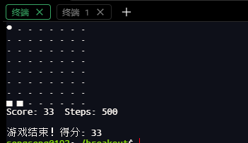
    cout << "\n游戏结束！得分: " << game.get_score() << endl;
    
    return 0;
}

训练过程

第 135 代, 最优适应度: 34.65 (停滞17代, 变异率=0.221618)
第 136 代, 最优适应度: 34.65 (停滞18代, 变异率=0.232699)
第 137 代, 最优适应度: 34.65 (停滞19代, 变异率=0.244334)
第 138 代, 最优适应度: 34.65 (停滞20代, 变异率=0.25)
【重置】长期停滞，重置最差的 20% 个体
第 139 代, 最优适应度: 34.65
第 140 代, 最优适应度: 34.65
模型已保存至 best_model.txt
第 141 代, 最优适应度: 34.65
第 142 代, 最优适应度: 34.65
第 143 代, 最优适应度: 34.65
第 144 代, 最优适应度: 34.65
第 145 代, 最优适应度: 34.65
第 146 代, 最优适应度: 34.65
第 147 代, 最优适应度: 34.65
第 148 代, 最优适应度: 34.65 (停滞10代, 变异率=0.1575)
第 149 代, 最优适应度: 34.65 (停滞11代, 变异率=0.165375)
第 150 代, 最优适应度: 34.65 (停滞12代, 变异率=0.173644)
模型已保存至 best_model.txt

训练完成！最优适应度: 34.65

演示最优个体游戏过程（自动运行 100 局）...

========== 演示统计 ==========
局数: 100
平均得分: 33.00
最高分: 33
最低分: 33
得分标准差: 0.00
得分为0的局数: 0 (0.00%)

得分分布:
  0分      : 0 局 (0.00%)
  1-10分   : 0 局 (0.00%)
  11-20分  : 0 局 (0.00%)
  21-30分  : 0 局 (0.00%)
  31-40分  : 100 局 (100.00%)
  41分以上 : 0 局 (0.00%)
==========================

演示效果：