基于BP神经网络的多变量时间序列预测 不调用工具箱函数 BP多变量时间序列 Matlab代码， 注：暂无Matlab版本要求 -- 推荐 2018B 版本及以上

最近在研究多变量时间序列预测，发现BP神经网络是个挺不错的方法。今天就来和大家分享一下基于BP神经网络的多变量时间序列预测的Matlab代码，而且全程不调用工具箱函数哦！

一、BP神经网络简介

BP神经网络是一种按误差反向传播算法训练的多层前馈网络，是目前应用最广泛的神经网络模型之一。它的基本结构包括输入层、隐藏层和输出层。在训练过程中，通过不断调整神经元之间的权重，使得预测值与真实值之间的误差最小化。

二、Matlab代码实现

% 清空工作区
clear all;
close all;
clc;

% 生成多变量时间序列数据
n = 100; % 数据长度
x1 = randn(n,1); % 变量1
x2 = randn(n,1); % 变量2
y = x1 + 2*x2 + 0.5*randn(n,1); % 目标变量

% 划分训练集和测试集
train_ratio = 0.8;
train_num = round(train_ratio * n);
x1_train = x1(1:train_num);
x2_train = x2(1:train_num);
y_train = y(1:train_num);
x1_test = x1(train_num+1:end);
x2_test = x2(train_num+1:end);
y_test = y(train_num+1:end);

% 初始化网络参数
input_size = 2; % 输入层神经元数量
hidden_size = 5; % 隐藏层神经元数量
output_size = 1; % 输出层神经元数量
learning_rate = 0.1; % 学习率
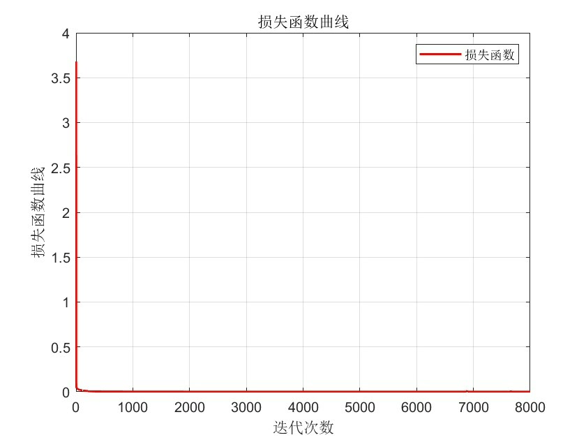
max_epoch = 1000; % 最大迭代次数

% 随机初始化权重
W1 = randn(hidden_size, input_size);
b1 = zeros(hidden_size, 1);
W2 = randn(output_size, hidden_size);
b2 = zeros(output_size, 1);

% BP神经网络训练
for epoch = 1:max_epoch
    % 前向传播
    z1 = W1 * [x1_train; x2_train] + b1;
    a1 = sigmoid(z1);
    z2 = W2 * a1 + b2;
    y_pred = sigmoid(z2);
    
    % 计算误差
    error = y_train - y_pred;
    
    % 反向传播
    d2 = error.* sigmoid_derivative(z2);
    d1 = W2' * d2.* sigmoid_derivative(z1);
    
    % 更新权重
    W2 = W2 + learning_rate * d2 * a1';
    b2 = b2 + learning_rate * sum(d2, 2);
    W1 = W1 + learning_rate * d1 * [x1_train; x2_train]';
    b1 = b1 + learning_rate * sum(d1, 2);
    
    % 打印误差
    if mod(epoch, 100) == 0
        mse = mean(error.^2);
        fprintf('Epoch %d, MSE: %f\n', epoch, mse);
    end
end

% 测试
z1 = W1 * [x1_test; x2_test] + b1;
a1 = sigmoid(z1);
z2 = W2 * a1 + b2;
y_pred_test = sigmoid(z2);

% 计算测试集误差
mse_test = mean((y_test - y_pred_test).^2);
fprintf('Test MSE: %f\n', mse_test);

% 定义激活函数sigmoid
function y = sigmoid(x)
    y = 1./(1 + exp(-x));
end

% 定义激活函数的导数
function y = sigmoid_derivative(x)
    y = sigmoid(x).*(1 - sigmoid(x));
end

三、代码分析

1. 数据生成与划分
   `matlab
   n = 100; % 数据长度
   x1 = randn(n,1); % 变量1
   x2 = randn(n,1); % 变量2
   y = x1 + 2x2 + 0.5randn(n,1); % 目标变量

train_ratio = 0.8;

trainnum = round(trainratio * n);

x1train = x1(1:trainnum);

x2train = x2(1:trainnum);

ytrain = y(1:trainnum);

x1test = x1(trainnum+1:end);

x2test = x2(trainnum+1:end);

ytest = y(trainnum+1:end);

`

这里生成了两个随机的变量x1和x2，并根据它们生成目标变量y。然后按照8:2的比例划分训练集和测试集。

1. 网络参数初始化
   `matlab
   inputsize = 2; % 输入层神经元数量
   hiddensize = 5; % 隐藏层神经元数量
   outputsize = 1; % 输出层神经元数量
   learningrate = 0.1; % 学习率
   max_epoch = 1000; % 最大迭代次数

W1 = randn(hiddensize, inputsize);

b1 = zeros(hidden_size, 1);

基于BP神经网络的多变量时间序列预测 不调用工具箱函数 BP多变量时间序列 Matlab代码， 注：暂无Matlab版本要求 -- 推荐 2018B 版本及以上

W2 = randn(outputsize, hiddensize);

b2 = zeros(output_size, 1);

`

初始化了网络的层数、神经元数量、学习率和最大迭代次数，并随机初始化了权重和偏置。

1. 前向传播
   matlab
z1 = W1 [x1train; x2train] + b1;
a1 = sigmoid(z1);
z2 = W2 a1 + b2;
y_pred = sigmoid(z2);

   依次计算输入层到隐藏层、隐藏层到输出层的加权和，并通过激活函数sigmoid得到预测值。

1. 误差计算与反向传播
   `matlab
   error = ytrain - ypred;

d2 = error.* sigmoid_derivative(z2);

d1 = W2' d2. sigmoid_derivative(z1);

`

计算预测值与真实值之间的误差，然后通过反向传播计算误差对权重和偏置的梯度。

1. 权重更新
   matlab
W2 = W2 + learningrate d2 a1';
b2 = b2 + learningrate sum(d2, 2);
W1 = W1 + learningrate d1 [x1train; x2train]';
b1 = b1 + learningrate sum(d1, 2);

   根据计算得到的梯度更新权重和偏置。

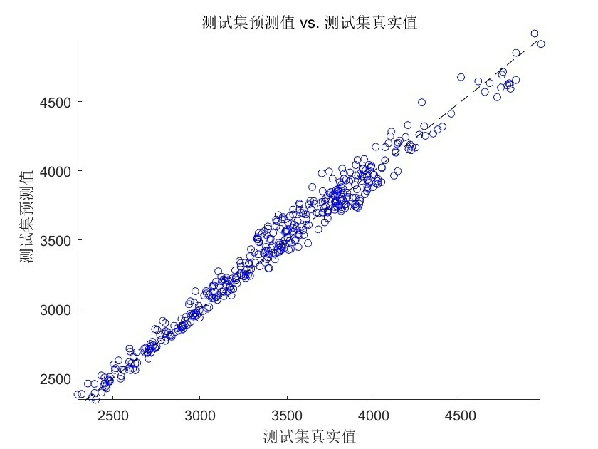
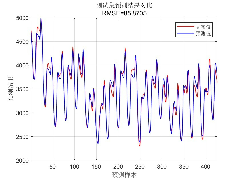
1. 测试
   `matlab
   z1 = W1 [x1test; x2test] + b1;
   a1 = sigmoid(z1);
   z2 = W2 a1 + b2;
   ypredtest = sigmoid(z2);

msetest = mean((ytest - ypredtest).^2);

fprintf('Test MSE: %f\n', mse_test);

`

使用训练好的网络对测试集进行预测，并计算测试集的均方误差。

通过这段代码，我们实现了基于BP神经网络的多变量时间序列预测，希望对大家有所帮助！如果有任何问题，欢迎留言讨论。