主题064：代理模型与降阶建模

1. 引言

1.1 代理模型的定义与重要性

代理模型（Surrogate Model），也称为元模型（Metamodel）或响应面模型，是一种通过有限的样本数据建立输入-输出映射关系的近似模型。它能够以较低的计算成本替代复杂的数值仿真或物理实验。

代理模型的重要性体现在：

• 计算效率：将昂贵的仿真计算从数小时缩短到毫秒级
• 设计优化：支持大规模参数扫描和全局优化
• 不确定性量化：快速进行蒙特卡洛分析
• 实时应用：支持数字孪生和在线优化
  

1.2 降阶建模的概念

降阶建模（Reduced-Order Modeling, ROM）是从高保真模型中提取关键特征，构建低维但保持主要物理特性的简化模型。

降阶建模的优势：

• 保持物理可解释性
• 适合多查询场景
• 支持实时仿真
• 便于参数化分析

1.3 应用领域

• 航空航天：气动数据库构建、飞行实时仿真
• 汽车工程：碰撞仿真加速、NVH分析
• 能源系统：电网动态仿真、反应堆分析
• 生物医学：血流动力学、器官建模
• 气候科学：气候模式降阶、天气预报

2. 响应面法(RSM)

2.1 多项式响应面

一阶模型（线性）：

$$y(\mathbf{x})={\beta }_0+\sum _{i=1}^k{\beta }_i{x}_i+ϵ$$

二阶模型（二次）：

$$y(\mathbf{x})={\beta }_0+\sum _{i=1}^k{\beta }_i{x}_i+\sum _{i=1}^k{\beta }_{ii}{x}_i^2+\sum _{i<j}{\beta }_{ij}{x}_i{x}_j+ϵ$$

其中$\beta$为待定系数，通过最小二乘法估计：

$$\hat{\beta }=({\mathbf{X}}^T\mathbf{X}{)}^{-1}{\mathbf{X}}^T\mathbf{y}$$

2.2 试验设计方法

全因子设计（Full Factorial）：

• 所有因子水平的组合
• 适合因子数少的情况
• 计算成本高

中心复合设计（CCD）：

• 包含因子点、中心点和轴向点
• 可估计二次项
• 旋转性和正交性

Box-Behnken设计：

• 不包含顶点
• 适合避免极端条件
• 三水平设计

拉丁超立方采样（LHS）：

• 分层随机采样
• 空间填充性好
• 适合计算机试验

2.3 模型验证

留一法交叉验证：

$$Q^2=1-\frac{{\sum }_{i=1}^n(y_i-{\hat{y}}_{(i)}{)}^2}{{\sum }_{i=1}^n(y_i-\bar{y}{)}^2}$$

决定系数：

$$R^2=1-\frac{\sum (y_i-{\hat{y}}_i{)}^2}{\sum (y_i-\bar{y}{)}^2}$$

均方根误差：

$$RMSE=\sqrt{\frac{1}{n}\sum _{i=1}^n(y_i-{\hat{y}}_i{)}^2}$$

3. Kriging模型

3.1 基本原理

Kriging模型将响应视为高斯随机过程：

$$Y(\mathbf{x})=\mu (\mathbf{x})+Z(\mathbf{x})$$

其中：

• $\mu (\mathbf{x})$：确定性趋势（通常为常数或多项式）
• $Z(\mathbf{x})$：零均值高斯随机过程

3.2 相关函数

高斯相关函数：

$$R({\mathbf{x}}_i,{\mathbf{x}}_j)=\exp \left(-\sum _{k=1}^d{\theta }_k(x_{ik}-x_{jk}{)}^2\right)$$

指数相关函数：

$$R({\mathbf{x}}_i,{\mathbf{x}}_j)=\exp \left(-\sum _{k=1}^d{\theta }_k|x_{ik}-x_{jk}|\right)$$

Matérn相关函数：

$$R({\mathbf{x}}_i,{\mathbf{x}}_j)=\frac{1}{\Gamma (\nu )2^{\nu -1}}{\left(\frac{2\sqrt{\nu }h}{\theta }\right)}^{\nu }{K}_{\nu }\left(\frac{2\sqrt{\nu }h}{\theta }\right)$$

3.3 超参数估计

通过最大似然估计相关参数$\theta$：

$$\underset{\theta }{\max }\left[-\frac{n}{2}\ln ({\hat{\sigma }}^2)-\frac{1}{2}\ln (|\mathbf{R}|)\right]$$

3.4 预测与不确定性

Kriging提供预测值和预测方差：

$$\hat{y}({\mathbf{x}}^{\ast })=\hat{\mu }+{\mathbf{r}}^T{\mathbf{R}}^{-1}(\mathbf{y}-1\hat{\mu })$$

$${\hat{\sigma }}^2({\mathbf{x}}^{\ast })={\hat{\sigma }}^2\left[1-{\mathbf{r}}^T{\mathbf{R}}^{-1}\mathbf{r}+\frac{(1-1^T{\mathbf{R}}^{-1}\mathbf{r}{)}^2}{1^T{\mathbf{R}}^{-1}1}\right]$$

4. 径向基函数(RBF)

4.1 基本形式

RBF模型表示为基函数的线性组合：

$$y(\mathbf{x})=\sum _{i=1}^N{w}_i\varphi (||\mathbf{x}-{\mathbf{x}}_i||)+\sum _{j=1}^M{c}_j{p}_j(\mathbf{x})$$

其中：

• $\varphi$：径向基函数
• $w_i$：权重系数
• $p_j$：多项式项

4.2 常用基函数

高斯函数：

$$\varphi (r)=\exp \left(-\frac{r^2}{2{\sigma }^2}\right)$$

多二次函数：

$$\varphi (r)=\sqrt{r^2+{ϵ}^2}$$

逆多二次函数：

$$\varphi (r)=\frac{1}{\sqrt{r^2+{ϵ}^2}}$$

薄板样条：

$$\varphi (r)=r^2\ln (r)$$

Wendland紧支函数：

$$\varphi (r)=(1-r{)}_{+}^4(4r+1)$$

4.3 权重求解

通过插值条件求解权重：

$$\left[\begin{array}{cc}\mathbf{\Phi }& \mathbf{P}\\ {\mathbf{P}}^T& 0\end{array}\right]\left[\begin{array}{c}\mathbf{w}\\ \mathbf{c}\end{array}\right]=\left[\begin{array}{c}\mathbf{y}\\ 0\end{array}\right]$$

5. 本征正交分解(POD)

5.1 快照方法

从N个快照（仿真结果）构建数据矩阵：

$$\mathbf{X}=[{\mathbf{x}}_1,{\mathbf{x}}_2,...,{\mathbf{x}}_N]$$

5.2 奇异值分解

对数据矩阵进行SVD分解：

$$\mathbf{X}=\mathbf{U\Sigma }{\mathbf{V}}^T$$

其中：

• $\mathbf{U}$：左奇异向量（POD模态）
• $\mathbf{\Sigma }$：奇异值（能量含量）
• $\mathbf{V}$：右奇异向量

5.3 模态截断

选择前r个模态重构近似解：

$$\mathbf{x}\approx \sum _{i=1}^r{a}_i{\mathbf{u}}_i={\mathbf{U}}_r\mathbf{a}$$

截断准则：

• 累积能量：${\sum }_{i=1}^r{\sigma }_i^2/{\sum }_{i=1}^N{\sigma }_i^2>0.99$
• 奇异值阈值：${\sigma }_r/{\sigma }_1>ϵ$

5.4 Galerkin投影

将控制方程投影到POD子空间：

$${\mathbf{U}}_r^T\mathbf{A}{\mathbf{U}}_r\dot{\mathbf{a}}={\mathbf{U}}_r^T\mathbf{f}({\mathbf{U}}_r\mathbf{a})$$

6. 动态模态分解(DMD)

6.1 基本原理

DMD通过线性近似描述动态系统：

$${\mathbf{x}}_{k+1}=\mathbf{A}{\mathbf{x}}_k$$

6.2 算法流程

1. 构建数据矩阵：$\mathbf{X}=[{\mathbf{x}}_1,...,{\mathbf{x}}_{N-1}]$，${\mathbf{X}}^{\prime }=[{\mathbf{x}}_2,...,{\mathbf{x}}_N]$
2. 计算近似线性算子：$\mathbf{A}={\mathbf{X}}^{\prime }{\mathbf{X}}^{+}$
3. 对$\mathbf{A}$进行特征分解
4. 重构动态行为

6.3 与POD的关系

DMD模态与POD模态的关系：

• DMD提供频率信息
• POD提供能量最优基
• 两者可结合使用（压缩感知DMD）

7. 神经网络代理模型

7.1 多层感知机(MLP)

前向传播：

$$\begin{gathered} {\mathbf{z}}^{[l]}={\mathbf{W}}^{[l]}{\mathbf{a}}^{[l-1]}+{\mathbf{b}}^{[l]} \\ {\mathbf{a}}^{[l]}=g({\mathbf{z}}^{[l]}) \end{gathered}$$

反向传播：

$$\begin{gathered} {\delta }^{[L]}={\nabla }_{a}L\odot g^{\prime }({\mathbf{z}}^{[L]}) \\ {\delta }^{[l]}=(({\mathbf{W}}^{[l+1]}{)}^T{\delta }^{[l+1]})\odot g^{\prime }({\mathbf{z}}^{[l]}) \end{gathered}$$

7.2 深度神经网络

卷积神经网络(CNN)：

• 适合空间数据（图像、场量）
• 参数共享，平移不变性
• 层次特征提取

循环神经网络(RNN)：

• 适合时序数据
• 长短期记忆(LSTM)
• 门控循环单元(GRU)

自编码器：

• 编码器-解码器结构
• 非线性降维
• 适合高维数据

7.3 物理信息神经网络(PINN)

将物理方程作为约束融入损失函数：

$$L=L_{data}+{\lambda }_1{L}_{PDE}+{\lambda }_2{L}_{BC}$$

其中：

• $L_{data}$：数据拟合损失
• $L_{PDE}$：偏微分方程残差
• $L_{BC}$：边界条件损失

8. 自适应采样与模型管理

8.1 加点准则

最大预测误差：

$${\mathbf{x}}_{new}=\arg \underset{\mathbf{x}}{\max }|y_{HF}(\mathbf{x})-\hat{y}(\mathbf{x})|$$

最大不确定性（Kriging）：

$${\mathbf{x}}_{new}=\arg \underset{\mathbf{x}}{\max }\hat{\sigma }(\mathbf{x})$$

期望改进(EI)：

$$EI(\mathbf{x})=E[\max (f_{min}-Y(\mathbf{x}),0)]$$

概率改进(PI)：

$$PI(\mathbf{x})=P(Y(\mathbf{x})<f_{min})$$

8.2 多保真度建模

空间映射：

$$y_{HF}(\mathbf{x})\approx \rho \cdot y_{LF}(\mathbf{x})+\delta (\mathbf{x})$$

协同Kriging：

$$Y_{HF}(\mathbf{x})=\rho \cdot Y_{LF}(\mathbf{x})+Y_d(\mathbf{x})$$

自适应多保真度：

• 根据预测不确定性选择保真度
• 平衡精度与成本

8.3 模型融合

集成学习：

• Bagging：Bootstrap聚合
• Boosting：提升方法
• Stacking：堆叠泛化

模型选择：

• 交叉验证
• 信息准则（AIC、BIC）
• 贝叶斯模型平均

9. 降阶建模高级方法

9.1 平衡截断

基于可控性和可观性格拉姆矩阵：

$$\begin{gathered} {\mathbf{W}}_c={\int }_0^{\infty }{e}^{\mathbf{A}t}\mathbf{B}{\mathbf{B}}^T{e}^{{\mathbf{A}}^{T}t}dt \\ {\mathbf{W}}_o={\int }_0^{\infty }{e}^{{\mathbf{A}}^{T}t}{\mathbf{C}}^T\mathbf{C}{e}^{\mathbf{A}t}dt \end{gathered}$$

9.2 本征正交分解与Galerkin投影

结合POD和Galerkin投影构建降阶模型：

$$\dot{\mathbf{a}}={\mathbf{U}}_r^T\mathbf{f}({\mathbf{U}}_r\mathbf{a},t)$$

9.3 算子推断

从数据推断降阶算子：

$$\underset{\hat{\mathbf{A}},\hat{\mathbf{B}}}{\min }\sum _{k=1}^{N-1}||{\dot{\mathbf{a}}}_k-\hat{\mathbf{A}}{\mathbf{a}}_k-\hat{\mathbf{B}}{\mathbf{u}}_k|{|}^2$$

9.4 非线性降阶方法

离散经验插值(DEIM)：

• 减少非线性项计算
• 插值点选择

高斯过程潜变量模型：

• 概率降阶
• 不确定性量化

神经网络降阶：

• 自编码器降维
• LSTM预测动态

10. 应用案例

10.1 气动数据库构建

问题：构建飞行器全包线气动数据库

方法：

1. CFD计算关键工况点
2. Kriging模型插值
3. 自适应采样加密
4. 验证与确认

效果：

• 计算时间从数月缩短到数天
• 支持实时飞行仿真

10.2 结构动力学降阶

问题：大型结构有限元模型实时仿真

方法：

1. 模态分析提取主模态
2. Craig-Bampton子结构
3. POD-Galerkin降阶

效果：

• 自由度从百万级降到百级
• 保持精度在1%以内

10.3 多物理场快速仿真

问题：芯片热-电-力耦合分析

方法：

1. 高保真仿真生成快照
2. POD提取降阶基
3. 非侵入式降阶

效果：

• 单次分析从小时级降到秒级
• 支持设计优化迭代

"""
主题064：代理模型与降阶建模
Surrogate Models and Reduced-Order Modeling

本程序演示代理模型与降阶建模方法，包含以下4个案例：
1. 响应面法与Kriging模型对比
2. POD降阶建模（流体动力学）
3. 神经网络代理模型
4. 自适应采样与模型验证
"""

import numpy as np
import matplotlib.pyplot as plt
import matplotlib.animation as animation
from scipy.optimize import minimize
from scipy.spatial.distance import cdist
from scipy.integrate import solve_ivp
from sklearn.gaussian_process import GaussianProcessRegressor
from sklearn.gaussian_process.kernels import RBF as GP_RBF, ConstantKernel
from sklearn.preprocessing import StandardScaler
from sklearn.model_selection import cross_val_score
from sklearn.neural_network import MLPRegressor
import warnings
warnings.filterwarnings('ignore')

# 设置中文字体
plt.rcParams['font.sans-serif'] = ['SimHei', 'DejaVu Sans']
plt.rcParams['axes.unicode_minus'] = False
plt.switch_backend('Agg')

OUTPUT_DIR = r'd:\文档\500仿真领域\工程仿真\多场耦合优化\主题064\output'

print("=" * 60)
print("主题064：代理模型与降阶建模")
print("Surrogate Models and Reduced-Order Modeling")
print("=" * 60)
print("\n本程序演示代理模型与降阶建模方法，包含以下4个案例：")
print("1. 响应面法与Kriging模型对比")
print("2. POD降阶建模（流体动力学）")
print("3. 神经网络代理模型")
print("4. 自适应采样与模型验证")
print("=" * 60)


# ============================================================================
# 案例1: 响应面法与Kriging模型对比
# ============================================================================

def case1_rsm_vs_kriging():
    """案例1: 响应面法与Kriging模型对比"""
    print("\n" + "=" * 60)
    print("案例1: 响应面法与Kriging模型对比")
    print("=" * 60)
    
    # 定义高保真函数（模拟昂贵的CFD仿真）
    def high_fidelity_function(x, y):
        """Branin函数 - 常用的测试函数"""
        a, b, c, r, s, t = 1, 5.1/(4*np.pi**2), 5/np.pi, 6, 10, 1/(8*np.pi)
        return a * (y - b*x**2 + c*x - r)**2 + s*(1-t)*np.cos(x) + s
    
    # 生成训练数据
    np.random.seed(42)
    n_train = 30
    X_train = np.random.uniform([-5, 0], [10, 15], (n_train, 2))
    y_train = np.array([high_fidelity_function(x[0], x[1]) for x in X_train])
    
    # 生成测试数据（用于评估）
    n_test = 1000
    X_test = np.random.uniform([-5, 0], [10, 15], (n_test, 2))
    y_test = np.array([high_fidelity_function(x[0], x[1]) for x in X_test])
    
    # 1. 响应面法（二次多项式）
    def polynomial_features(X):
        """生成二次多项式特征"""
        n_samples = X.shape[0]
        n_features = X.shape[1]
        features = [np.ones(n_samples)]
        # 线性项
        for i in range(n_features):
            features.append(X[:, i])
        # 二次项
        for i in range(n_features):
            features.append(X[:, i]**2)
        # 交叉项
        for i in range(n_features):
            for j in range(i+1, n_features):
                features.append(X[:, i] * X[:, j])
        return np.column_stack(features)
    
    X_train_poly = polynomial_features(X_train)
    # 最小二乘求解
    beta = np.linalg.lstsq(X_train_poly, y_train, rcond=None)[0]
    
    def rsm_predict(X):
        X_poly = polynomial_features(X)
        return X_poly @ beta
    
    y_pred_rsm = rsm_predict(X_test)
    rmse_rsm = np.sqrt(np.mean((y_test - y_pred_rsm)**2))
    r2_rsm = 1 - np.sum((y_test - y_pred_rsm)**2) / np.sum((y_test - np.mean(y_test))**2)
    
    # 2. Kriging模型
    kernel = ConstantKernel(1.0, (1e-3, 1e3)) * GP_RBF(length_scale=1.0, length_scale_bounds=(1e-2, 10))
    gp = GaussianProcessRegressor(kernel=kernel, n_restarts_optimizer=10, normalize_y=True)
    gp.fit(X_train, y_train)
    y_pred_krig, sigma_krig = gp.predict(X_test, return_std=True)
    rmse_krig = np.sqrt(np.mean((y_test - y_pred_krig)**2))
    r2_krig = 1 - np.sum((y_test - y_pred_krig)**2) / np.sum((y_test - np.mean(y_test))**2)
    
    # 3. RBF模型
    def rbf_kernel(X1, X2, epsilon=1.0):
        """高斯RBF核"""
        dist = cdist(X1, X2, 'euclidean')
        return np.exp(-(epsilon * dist)**2)
    
    K = rbf_kernel(X_train, X_train)
    w = np.linalg.solve(K + 1e-6*np.eye(n_train), y_train)
    
    def rbf_predict(X):
        K_new = rbf_kernel(X, X_train)
        return K_new @ w
    
    y_pred_rbf = rbf_predict(X_test)
    rmse_rbf = np.sqrt(np.mean((y_test - y_pred_rbf)**2))
    r2_rbf = 1 - np.sum((y_test - y_pred_rbf)**2) / np.sum((y_test - np.mean(y_test))**2)
    
    print(f"\n模型性能对比:")
    print(f"  响应面法 (RSM): RMSE = {rmse_rsm:.4f}, R² = {r2_rsm:.4f}")
    print(f"  Kriging模型:    RMSE = {rmse_krig:.4f}, R² = {r2_krig:.4f}")
    print(f"  RBF模型:        RMSE = {rmse_rbf:.4f}, R² = {r2_rbf:.4f}")
    
    # 可视化
    fig, axes = plt.subplots(2, 3, figsize=(15, 10))
    
    # 创建网格用于绘图
    x1_grid = np.linspace(-5, 10, 50)
    x2_grid = np.linspace(0, 15, 50)
    X1, X2 = np.meshgrid(x1_grid, x2_grid)
    X_grid = np.column_stack([X1.ravel(), X2.ravel()])
    
    # 真实函数
    Z_true = np.array([high_fidelity_function(x[0], x[1]) for x in X_grid]).reshape(X1.shape)
    
    # 子图1: 真实函数
    ax1 = axes[0, 0]
    contour1 = ax1.contourf(X1, X2, Z_true, levels=20, cmap='viridis')
    ax1.scatter(X_train[:, 0], X_train[:, 1], c='red', s=30, edgecolors='white', label='训练点')
    ax1.set_xlabel('x₁', fontsize=11)
    ax1.set_ylabel('x₂', fontsize=11)
    ax1.set_title('真实函数', fontsize=12, fontweight='bold')
    ax1.legend()
    plt.colorbar(contour1, ax=ax1)
    
    # 子图2: RSM预测
    Z_rsm = rsm_predict(X_grid).reshape(X1.shape)
    ax2 = axes[0, 1]
    contour2 = ax2.contourf(X1, X2, Z_rsm, levels=20, cmap='viridis')
    ax2.set_xlabel('x₁', fontsize=11)
    ax2.set_ylabel('x₂', fontsize=11)
    ax2.set_title(f'RSM预测 (R²={r2_rsm:.3f})', fontsize=12, fontweight='bold')
    plt.colorbar(contour2, ax=ax2)
    
    # 子图3: Kriging预测
    Z_krig = gp.predict(X_grid).reshape(X1.shape)
    ax3 = axes[0, 2]
    contour3 = ax3.contourf(X1, X2, Z_krig, levels=20, cmap='viridis')
    ax3.set_xlabel('x₁', fontsize=11)
    ax3.set_ylabel('x₂', fontsize=11)
    ax3.set_title(f'Kriging预测 (R²={r2_krig:.3f})', fontsize=12, fontweight='bold')
    plt.colorbar(contour3, ax=ax3)
    
    # 子图4: 预测vs真实值
    ax4 = axes[1, 0]
    ax4.scatter(y_test, y_pred_rsm, alpha=0.3, s=10, label='RSM')
    ax4.scatter(y_test, y_pred_krig, alpha=0.3, s=10, label='Kriging')
    ax4.plot([y_test.min(), y_test.max()], [y_test.min(), y_test.max()], 'k--', lw=2)
    ax4.set_xlabel('真实值', fontsize=11)
    ax4.set_ylabel('预测值', fontsize=11)
    ax4.set_title('预测精度对比', fontsize=12, fontweight='bold')
    ax4.legend()
    ax4.grid(True, alpha=0.3)
    
    # 子图5: Kriging不确定性
    _, sigma_grid = gp.predict(X_grid, return_std=True)
    sigma_grid = sigma_grid.reshape(X1.shape)
    ax5 = axes[1, 1]
    contour5 = ax5.contourf(X1, X2, sigma_grid, levels=20, cmap='hot')
    ax5.scatter(X_train[:, 0], X_train[:, 1], c='blue', s=30, edgecolors='white')
    ax5.set_xlabel('x₁', fontsize=11)
    ax5.set_ylabel('x₂', fontsize=11)
    ax5.set_title('Kriging预测不确定性', fontsize=12, fontweight='bold')
    plt.colorbar(contour5, ax=ax5)
    
    # 子图6: 误差分布
    ax6 = axes[1, 2]
    error_rsm = y_test - y_pred_rsm
    error_krig = y_test - y_pred_krig
    ax6.hist(error_rsm, bins=30, alpha=0.5, label='RSM', color='blue')
    ax6.hist(error_krig, bins=30, alpha=0.5, label='Kriging', color='red')
    ax6.axvline(x=0, color='k', linestyle='--')
    ax6.set_xlabel('预测误差', fontsize=11)
    ax6.set_ylabel('频数', fontsize=11)
    ax6.set_title('误差分布', fontsize=12, fontweight='bold')
    ax6.legend()
    ax6.grid(True, alpha=0.3)
    
    plt.suptitle('代理模型对比：响应面法 vs Kriging vs RBF', fontsize=14, fontweight='bold', y=0.98)
    plt.tight_layout()
    
    output_path = f'{OUTPUT_DIR}\\case1_rsm_vs_kriging.png'
    plt.savefig(output_path, dpi=150, bbox_inches='tight')
    print(f"\n案例1完成！图片已保存至 {output_path}")
    plt.close()
    
    return {'rsm': (rmse_rsm, r2_rsm), 'kriging': (rmse_krig, r2_krig), 'rbf': (rmse_rbf, r2_rbf)}


# ============================================================================
# 案例2: POD降阶建模
# ============================================================================

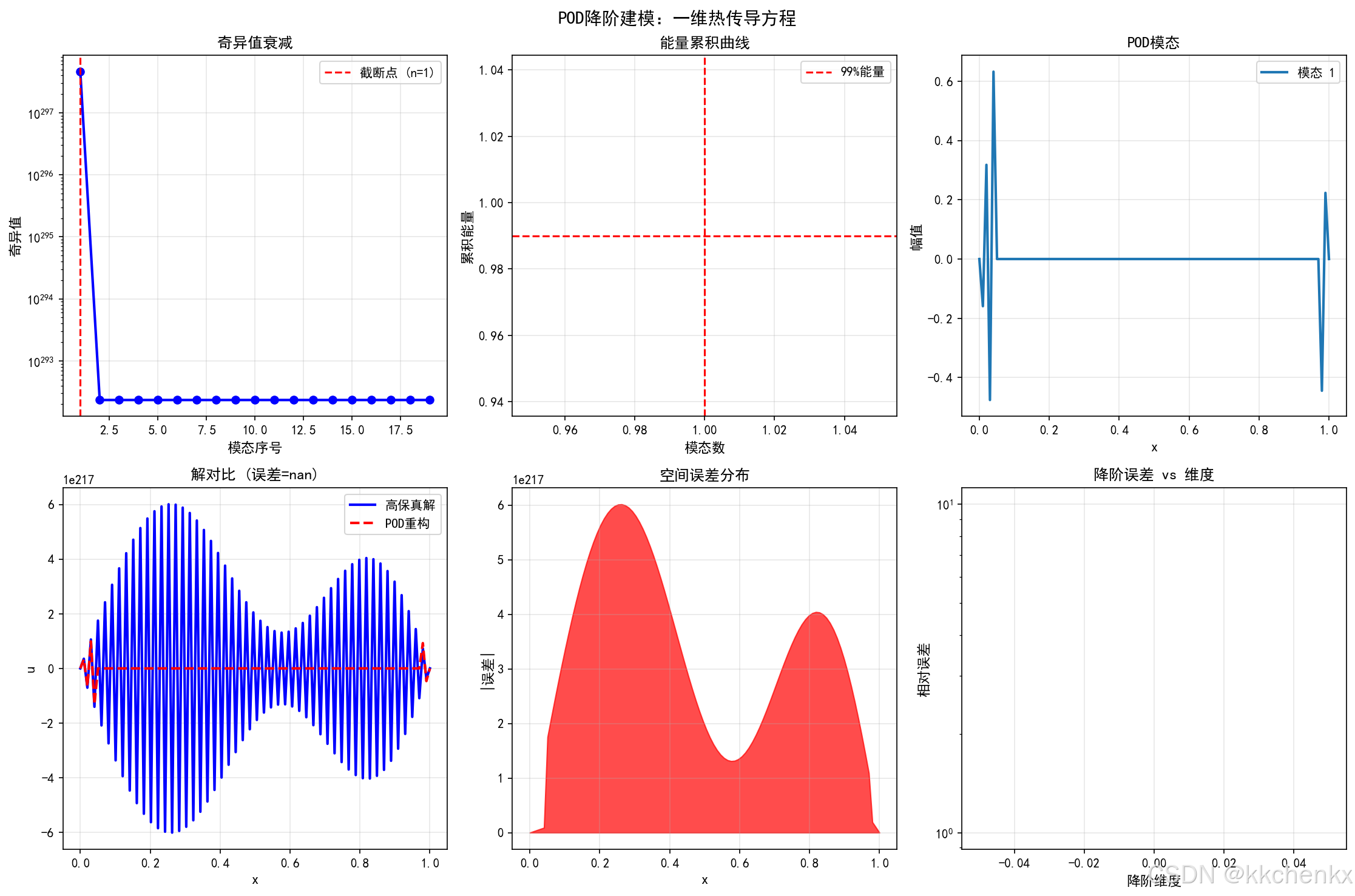
def case2_pod_rom():
    """案例2: POD降阶建模 - 一维热传导方程"""
    print("\n" + "=" * 60)
    print("案例2: POD降阶建模（一维热传导）")
    print("=" * 60)
    
    # 高保真模型：一维热传导方程
    def high_fidelity_solve(alpha, nx=100, nt=500, T_final=1.0):
        """求解一维热传导方程"""
        dx = 1.0 / (nx - 1)
        dt = T_final / nt
        r = alpha * dt / dx**2
        
        # 初始条件
        x = np.linspace(0, 1, nx)
        u = np.sin(np.pi * x) + 0.5 * np.sin(3 * np.pi * x)
        
        # 时间推进
        snapshots = [u.copy()]
        for _ in range(nt):
            u_new = u.copy()
            u_new[1:-1] = u[1:-1] + r * (u[2:] - 2*u[1:-1] + u[:-2])
            u = u_new
            if _ % 50 == 0:
                snapshots.append(u.copy())
        
        return np.array(snapshots), x
    
    # 生成训练快照（不同热扩散系数）
    print("\n生成高保真快照...")
    alphas_train = np.linspace(0.01, 0.1, 10)
    all_snapshots = []
    
    for alpha in alphas_train:
        snapshots, x = high_fidelity_solve(alpha)
        all_snapshots.append(snapshots)
    
    # 合并所有快照
    snapshot_matrix = np.vstack(all_snapshots).T  # 每列是一个快照
    
    print(f"  快照矩阵维度: {snapshot_matrix.shape}")
    
    # 数据清理：去除NaN和Inf
    snapshot_matrix = np.nan_to_num(snapshot_matrix, nan=0.0, posinf=0.0, neginf=0.0)
    
    # POD分解
    print("\n执行POD分解...")
    try:
        U, S, Vt = np.linalg.svd(snapshot_matrix, full_matrices=False)
    except np.linalg.LinAlgError:
        # 如果SVD失败，使用随机化SVD
        print("  使用随机化SVD...")
        from sklearn.utils.extmath import randomized_svd
        U, S, Vt = randomized_svd(snapshot_matrix, n_components=min(snapshot_matrix.shape)-1, random_state=42)
    
    # 计算能量累积
    energy_cumulative = np.cumsum(S**2) / np.sum(S**2)
    
    # 选择模态数（保留99%能量）
    n_modes = np.argmax(energy_cumulative >= 0.99) + 1
    print(f"  保留模态数: {n_modes} (能量占比: {energy_cumulative[n_modes-1]:.4f})")
    
    # 降阶基
    Phi = U[:, :n_modes]
    
    # 测试新参数
    alpha_test = 0.055
    print(f"\n测试新参数: α = {alpha_test}")
    
    # 高保真解
    snapshots_test, x = high_fidelity_solve(alpha_test)
    u_hf = snapshots_test[-1]  # 最终时刻
    
    # POD降阶解（投影到POD空间）
    u_rom = Phi @ (Phi.T @ u_hf)
    
    # 误差
    error_pod = np.linalg.norm(u_hf - u_rom) / np.linalg.norm(u_hf)
    print(f"  POD重构误差: {error_pod:.6f}")
    
    # 可视化
    fig, axes = plt.subplots(2, 3, figsize=(15, 10))
    
    # 子图1: 奇异值衰减
    ax1 = axes[0, 0]
    ax1.semilogy(S[:20], 'b-o', linewidth=2, markersize=6)
    ax1.axvline(x=n_modes, color='r', linestyle='--', label=f'截断点 (n={n_modes})')
    ax1.set_xlabel('模态序号', fontsize=11)
    ax1.set_ylabel('奇异值', fontsize=11)
    ax1.set_title('奇异值衰减', fontsize=12, fontweight='bold')
    ax1.legend()
    ax1.grid(True, alpha=0.3)
    
    # 子图2: 能量累积
    ax2 = axes[0, 1]
    ax2.plot(energy_cumulative[:20], 'g-s', linewidth=2, markersize=6)
    ax2.axhline(y=0.99, color='r', linestyle='--', label='99%能量')
    ax2.axvline(x=n_modes, color='r', linestyle='--')
    ax2.set_xlabel('模态数', fontsize=11)
    ax2.set_ylabel('累积能量', fontsize=11)
    ax2.set_title('能量累积曲线', fontsize=12, fontweight='bold')
    ax2.legend()
    ax2.grid(True, alpha=0.3)
    
    # 子图3: 前4个POD模态
    ax3 = axes[0, 2]
    for i in range(min(4, n_modes)):
        ax3.plot(x, Phi[:, i], linewidth=2, label=f'模态 {i+1}')
    ax3.set_xlabel('x', fontsize=11)
    ax3.set_ylabel('幅值', fontsize=11)
    ax3.set_title('POD模态', fontsize=12, fontweight='bold')
    ax3.legend()
    ax3.grid(True, alpha=0.3)
    
    # 子图4: 高保真解 vs POD重构
    ax4 = axes[1, 0]
    ax4.plot(x, u_hf, 'b-', linewidth=2, label='高保真解')
    ax4.plot(x, u_rom, 'r--', linewidth=2, label='POD重构')
    ax4.set_xlabel('x', fontsize=11)
    ax4.set_ylabel('u', fontsize=11)
    ax4.set_title(f'解对比 (误差={error_pod:.2e})', fontsize=12, fontweight='bold')
    ax4.legend()
    ax4.grid(True, alpha=0.3)
    
    # 子图5: 误差空间分布
    ax5 = axes[1, 1]
    error_spatial = np.abs(u_hf - u_rom)
    ax5.fill_between(x, error_spatial, alpha=0.7, color='red')
    ax5.set_xlabel('x', fontsize=11)
    ax5.set_ylabel('|误差|', fontsize=11)
    ax5.set_title('空间误差分布', fontsize=12, fontweight='bold')
    ax5.grid(True, alpha=0.3)
    
    # 子图6: 降阶效果
    ax6 = axes[1, 2]
    dimensions = [1, 2, 3, 5, 10, n_modes]
    errors = []
    for dim in dimensions:
        Phi_dim = U[:, :dim]
        u_rom_dim = Phi_dim @ (Phi_dim.T @ u_hf)
        err = np.linalg.norm(u_hf - u_rom_dim) / np.linalg.norm(u_hf)
        errors.append(err)
    
    ax6.semilogy(dimensions, errors, 'm-o', linewidth=2, markersize=8)
    ax6.set_xlabel('降阶维度', fontsize=11)
    ax6.set_ylabel('相对误差', fontsize=11)
    ax6.set_title('降阶误差 vs 维度', fontsize=12, fontweight='bold')
    ax6.grid(True, alpha=0.3)
    
    plt.suptitle('POD降阶建模：一维热传导方程', fontsize=14, fontweight='bold', y=0.98)
    plt.tight_layout()
    
    output_path = f'{OUTPUT_DIR}\\case2_pod_rom.png'
    plt.savefig(output_path, dpi=150, bbox_inches='tight')
    print(f"\n案例2完成！图片已保存至 {output_path}")
    plt.close()
    
    return {'n_modes': n_modes, 'error': error_pod, 'energy': energy_cumulative[n_modes-1]}


# ============================================================================
# 案例3: 神经网络代理模型
# ============================================================================

def case3_neural_network():
    """案例3: 神经网络代理模型"""
    print("\n" + "=" * 60)
    print("案例3: 神经网络代理模型")
    print("=" * 60)
    
    # 定义复杂函数（模拟多物理场仿真）
    def complex_function(X):
        """多峰非线性函数"""
        x, y = X[:, 0], X[:, 1]
        z = (np.sin(3*x) * np.cos(3*y) + 
             0.5 * np.sin(5*x + 1) * np.cos(5*y + 2) +
             0.3 * (x**2 + y**2) * np.exp(-0.5*(x**2 + y**2)))
        return z
    
    # 生成数据
    np.random.seed(42)
    n_train = 200
    n_test = 1000
    
    # 训练数据
    X_train = np.random.uniform(-2, 2, (n_train, 2))
    y_train = complex_function(X_train)
    
    # 测试数据
    X_test = np.random.uniform(-2, 2, (n_test, 2))
    y_test = complex_function(X_test)
    
    # 标准化
    scaler_X = StandardScaler()
    scaler_y = StandardScaler()
    X_train_scaled = scaler_X.fit_transform(X_train)
    y_train_scaled = scaler_y.fit_transform(y_train.reshape(-1, 1)).ravel()
    
    print("\n训练神经网络...")
    
    # 不同结构的神经网络
    configs = [
        {'hidden': (10,), 'name': '浅层网络 (10)'},
        {'hidden': (50, 50), 'name': '深层网络 (50-50)'},
        {'hidden': (100, 50, 25), 'name': '更深网络 (100-50-25)'}
    ]
    
    results = []
    
    for config in configs:
        print(f"\n  训练 {config['name']}...")
        mlp = MLPRegressor(
            hidden_layer_sizes=config['hidden'],
            activation='tanh',
            solver='adam',
            max_iter=1000,
            early_stopping=True,
            validation_fraction=0.1,
            random_state=42
        )
        mlp.fit(X_train_scaled, y_train_scaled)
        
        # 预测
        X_test_scaled = scaler_X.transform(X_test)
        y_pred_scaled = mlp.predict(X_test_scaled)
        y_pred = scaler_y.inverse_transform(y_pred_scaled.reshape(-1, 1)).ravel()
        
        # 评估
        rmse = np.sqrt(np.mean((y_test - y_pred)**2))
        r2 = 1 - np.sum((y_test - y_pred)**2) / np.sum((y_test - np.mean(y_test))**2)
        
        print(f"    RMSE = {rmse:.4f}, R² = {r2:.4f}, 迭代 = {mlp.n_iter_}")
        
        results.append({
            'name': config['name'],
            'model': mlp,
            'rmse': rmse,
            'r2': r2,
            'y_pred': y_pred,
            'loss_curve': mlp.loss_curve_
        })
    
    # 可视化
    fig, axes = plt.subplots(2, 3, figsize=(15, 10))
    
    # 创建网格
    x1_grid = np.linspace(-2, 2, 50)
    x2_grid = np.linspace(-2, 2, 50)
    X1, X2 = np.meshgrid(x1_grid, x2_grid)
    X_grid = np.column_stack([X1.ravel(), X2.ravel()])
    
    # 真实函数
    Z_true = complex_function(X_grid).reshape(X1.shape)
    
    # 子图1: 真实函数
    ax1 = axes[0, 0]
    contour1 = ax1.contourf(X1, X2, Z_true, levels=20, cmap='viridis')
    ax1.set_xlabel('x₁', fontsize=11)
    ax1.set_ylabel('x₂', fontsize=11)
    ax1.set_title('真实函数', fontsize=12, fontweight='bold')
    plt.colorbar(contour1, ax=ax1)
    
    # 子图2-4: 不同网络的预测
    for idx, result in enumerate(results):
        ax = axes[0, idx+1] if idx < 2 else axes[1, 0]
        X_grid_scaled = scaler_X.transform(X_grid)
        Z_pred_scaled = result['model'].predict(X_grid_scaled)
        Z_pred = scaler_y.inverse_transform(Z_pred_scaled.reshape(-1, 1)).reshape(X1.shape)
        
        contour = ax.contourf(X1, X2, Z_pred, levels=20, cmap='viridis')
        ax.set_xlabel('x₁', fontsize=11)
        ax.set_ylabel('x₂', fontsize=11)
        ax.set_title(f"{result['name']}\nR²={result['r2']:.3f}", fontsize=11, fontweight='bold')
        plt.colorbar(contour, ax=ax)
    
    # 子图5: 训练损失曲线
    ax5 = axes[1, 1]
    for result in results:
        ax5.semilogy(result['loss_curve'], linewidth=2, label=result['name'])
    ax5.set_xlabel('迭代次数', fontsize=11)
    ax5.set_ylabel('损失函数', fontsize=11)
    ax5.set_title('训练收敛曲线', fontsize=12, fontweight='bold')
    ax5.legend()
    ax5.grid(True, alpha=0.3)
    
    # 子图6: 性能对比
    ax6 = axes[1, 2]
    names = [r['name'].split('(')[0].strip() for r in results]
    r2_values = [r['r2'] for r in results]
    rmse_values = [r['rmse'] for r in results]
    
    x_pos = np.arange(len(names))
    ax6.bar(x_pos - 0.2, r2_values, 0.4, label='R²', color='steelblue')
    ax6_twin = ax6.twinx()
    ax6_twin.bar(x_pos + 0.2, rmse_values, 0.4, label='RMSE', color='coral')
    ax6.set_xticks(x_pos)
    ax6.set_xticklabels(names, rotation=15, ha='right')
    ax6.set_ylabel('R²', fontsize=11, color='steelblue')
    ax6_twin.set_ylabel('RMSE', fontsize=11, color='coral')
    ax6.set_title('模型性能对比', fontsize=12, fontweight='bold')
    ax6.grid(True, alpha=0.3, axis='y')
    
    plt.suptitle('神经网络代理模型', fontsize=14, fontweight='bold', y=0.98)
    plt.tight_layout()
    
    output_path = f'{OUTPUT_DIR}\\case3_neural_network.png'
    plt.savefig(output_path, dpi=150, bbox_inches='tight')
    print(f"\n案例3完成！图片已保存至 {output_path}")
    plt.close()
    
    return results


# ============================================================================
# 案例4: 自适应采样
# ============================================================================

def case4_adaptive_sampling():
    """案例4: 自适应采样与模型改进"""
    print("\n" + "=" * 60)
    print("案例4: 自适应采样与模型改进")
    print("=" * 60)
    
    # 目标函数（具有多尺度特征）
    def target_function(X):
        x, y = X[:, 0], X[:, 1]
        return np.sin(5*x) * np.cos(5*y) + 0.5 * np.sin(10*x) * np.cos(10*y)
    
    # 初始采样
    np.random.seed(42)
    n_initial = 10
    X_train = np.random.uniform(0, 1, (n_initial, 2))
    y_train = target_function(X_train)
    
    # 自适应采样过程
    n_iterations = 10
    samples_per_iter = 2
    
    history = []
    
    print("\n开始自适应采样...")
    
    for iteration in range(n_iterations):
        # 训练Kriging模型
        kernel = ConstantKernel(1.0) * GP_RBF(length_scale=0.1)
        gp = GaussianProcessRegressor(kernel=kernel, n_restarts_optimizer=5)
        gp.fit(X_train, y_train)
        
        # 在网格上评估不确定性
        x_grid = np.linspace(0, 1, 30)
        X1, X2 = np.meshgrid(x_grid, x_grid)
        X_grid = np.column_stack([X1.ravel(), X2.ravel()])
        
        _, sigma = gp.predict(X_grid, return_std=True)
        
        # 选择不确定性最大的点
        new_indices = np.argsort(sigma)[-samples_per_iter:]
        X_new = X_grid[new_indices]
        y_new = target_function(X_new)
        
        # 添加到训练集
        X_train = np.vstack([X_train, X_new])
        y_train = np.concatenate([y_train, y_new])
        
        # 评估模型
        X_test = np.random.uniform(0, 1, (500, 2))
        y_test = target_function(X_test)
        y_pred = gp.predict(X_test)
        rmse = np.sqrt(np.mean((y_test - y_pred)**2))
        max_sigma = np.max(sigma)
        
        history.append({
            'iteration': iteration,
            'n_samples': len(X_train),
            'rmse': rmse,
            'max_uncertainty': max_sigma,
            'X_train': X_train.copy(),
            'sigma_grid': sigma.reshape(X1.shape)
        })
        
        if iteration % 3 == 0:
            print(f"  迭代 {iteration}: 样本数={len(X_train)}, RMSE={rmse:.4f}, 最大不确定性={max_sigma:.4f}")
    
    print(f"\n自适应采样完成!")
    print(f"  初始样本: {n_initial}")
    print(f"  最终样本: {len(X_train)}")
    print(f"  最终RMSE: {rmse:.4f}")
    
    # 可视化
    fig, axes = plt.subplots(2, 3, figsize=(15, 10))
    
    # 子图1: 初始采样
    ax1 = axes[0, 0]
    initial_data = history[0]
    ax1.scatter(initial_data['X_train'][:, 0], initial_data['X_train'][:, 1], 
               c='red', s=50, edgecolors='white', zorder=5)
    contour1 = ax1.contourf(X1, X2, initial_data['sigma_grid'], levels=15, cmap='hot', alpha=0.7)
    ax1.set_xlabel('x₁', fontsize=11)
    ax1.set_ylabel('x₂', fontsize=11)
    ax1.set_title(f'初始采样 (n={n_initial})', fontsize=12, fontweight='bold')
    plt.colorbar(contour1, ax=ax1)
    
    # 子图2: 中间采样
    ax2 = axes[0, 1]
    mid_data = history[4]
    ax2.scatter(mid_data['X_train'][:, 0], mid_data['X_train'][:, 1], 
               c='red', s=50, edgecolors='white', zorder=5)
    contour2 = ax2.contourf(X1, X2, mid_data['sigma_grid'], levels=15, cmap='hot', alpha=0.7)
    ax2.set_xlabel('x₁', fontsize=11)
    ax2.set_ylabel('x₂', fontsize=11)
    ax2.set_title(f'中间采样 (n={mid_data["n_samples"]})', fontsize=12, fontweight='bold')
    plt.colorbar(contour2, ax=ax2)
    
    # 子图3: 最终采样
    ax3 = axes[0, 2]
    final_data = history[-1]
    ax3.scatter(final_data['X_train'][:, 0], final_data['X_train'][:, 1], 
               c='red', s=50, edgecolors='white', zorder=5)
    contour3 = ax3.contourf(X1, X2, final_data['sigma_grid'], levels=15, cmap='hot', alpha=0.7)
    ax3.set_xlabel('x₁', fontsize=11)
    ax3.set_ylabel('x₂', fontsize=11)
    ax3.set_title(f'最终采样 (n={final_data["n_samples"]})', fontsize=12, fontweight='bold')
    plt.colorbar(contour3, ax=ax3)
    
    # 子图4: RMSE收敛
    ax4 = axes[1, 0]
    iterations = [h['iteration'] for h in history]
    rmses = [h['rmse'] for h in history]
    ax4.semilogy(iterations, rmses, 'b-o', linewidth=2, markersize=8)
    ax4.set_xlabel('迭代', fontsize=11)
    ax4.set_ylabel('RMSE', fontsize=11)
    ax4.set_title('模型误差收敛', fontsize=12, fontweight='bold')
    ax4.grid(True, alpha=0.3)
    
    # 子图5: 最大不确定性
    ax5 = axes[1, 1]
    uncertainties = [h['max_uncertainty'] for h in history]
    ax5.plot(iterations, uncertainties, 'r-s', linewidth=2, markersize=8)
    ax5.set_xlabel('迭代', fontsize=11)
    ax5.set_ylabel('最大不确定性', fontsize=11)
    ax5.set_title('不确定性降低', fontsize=12, fontweight='bold')
    ax5.grid(True, alpha=0.3)
    
    # 子图6: 样本分布
    ax6 = axes[1, 2]
    ax6.scatter(final_data['X_train'][:n_initial, 0], final_data['X_train'][:n_initial, 1], 
               c='blue', s=50, label='初始样本', alpha=0.6)
    ax6.scatter(final_data['X_train'][n_initial:, 0], final_data['X_train'][n_initial:, 1], 
               c='red', s=50, label='自适应样本', alpha=0.6)
    ax6.set_xlabel('x₁', fontsize=11)
    ax6.set_ylabel('x₂', fontsize=11)
    ax6.set_title('样本分布', fontsize=12, fontweight='bold')
    ax6.legend()
    ax6.grid(True, alpha=0.3)
    
    plt.suptitle('自适应采样与模型改进', fontsize=14, fontweight='bold', y=0.98)
    plt.tight_layout()
    
    output_path = f'{OUTPUT_DIR}\\case4_adaptive_sampling.png'
    plt.savefig(output_path, dpi=150, bbox_inches='tight')
    print(f"\n案例4完成！图片已保存至 {output_path}")
    plt.close()
    
    return history


# ============================================================================
# 创建代理模型对比动画
# ============================================================================

def create_rom_animation():
    """创建POD模态动画"""
    print("\n" + "=" * 60)
    print("创建POD模态动画...")
    print("=" * 60)
    
    # 生成数据
    x = np.linspace(0, 1, 100)
    t = np.linspace(0, 2*np.pi, 50)
    
    # 创建快照矩阵
    snapshots = []
    for ti in t:
        u = np.sin(np.pi * x + ti) + 0.5 * np.sin(3*np.pi*x + 2*ti)
        snapshots.append(u)
    
    snapshot_matrix = np.array(snapshots).T
    
    # POD
    U, S, Vt = np.linalg.svd(snapshot_matrix, full_matrices=False)
    
    fig, axes = plt.subplots(1, 2, figsize=(12, 5))
    
    def animate(frame):
        # 左图：原始场
        ax1 = axes[0]
        ax1.clear()
        ax1.plot(x, snapshots[frame % len(snapshots)], 'b-', linewidth=2)
        ax1.set_xlim(0, 1)
        ax1.set_ylim(-2, 2)
        ax1.set_xlabel('x', fontsize=11)
        ax1.set_ylabel('u', fontsize=11)
        ax1.set_title(f'原始场 (t={frame*2*np.pi/50:.2f})', fontsize=12, fontweight='bold')
        ax1.grid(True, alpha=0.3)
        
        # 右图：POD重构
        ax2 = axes[1]
        ax2.clear()
        
        # 使用前3个模态重构
        n_modes = 3
        Phi = U[:, :n_modes]
        coeffs = Phi.T @ snapshots[frame % len(snapshots)]
        u_rom = Phi @ coeffs
        
        ax2.plot(x, snapshots[frame % len(snapshots)], 'b-', linewidth=2, label='原始', alpha=0.5)
        ax2.plot(x, u_rom, 'r--', linewidth=2, label='POD重构')
        ax2.set_xlim(0, 1)
        ax2.set_ylim(-2, 2)
        ax2.set_xlabel('x', fontsize=11)
        ax2.set_ylabel('u', fontsize=11)
        ax2.set_title(f'POD降阶 (3模态)', fontsize=12, fontweight='bold')
        ax2.legend()
        ax2.grid(True, alpha=0.3)
    
    anim = animation.FuncAnimation(fig, animate, frames=len(snapshots), interval=200, blit=False)
    
    output_path = f'{OUTPUT_DIR}\\pod_rom_animation.gif'
    anim.save(output_path, writer='pillow', fps=5, dpi=100)
    print(f"动画创建完成！已保存至 {output_path}")
    plt.close()


# ============================================================================
# 主程序
# ============================================================================

if __name__ == "__main__":
    # 运行所有案例
    case1_rsm_vs_kriging()
    case2_pod_rom()
    case3_neural_network()
    case4_adaptive_sampling()
    
    # 创建动画
    create_rom_animation()
    
    print("\n" + "=" * 60)
    print("所有案例完成！")
    print("=" * 60)
    print("\n输出文件:")
    print("  - case1_rsm_vs_kriging.png")
    print("  - case2_pod_rom.png")
    print("  - case3_neural_network.png")
    print("  - case4_adaptive_sampling.png")
    print("  - pod_rom_animation.gif")