1、iris数据集训练模型

# 安装
#install.packages("randomForest")
#install.packages("ranger")

# 加载
library(randomForest)
library(ranger)
data(iris)
# 划分训练集70%、测试集30%
set.seed(123) # 固定随机种子，结果可复现
train_idx <- sample(1:nrow(iris), 0.7*nrow(iris))
train <- iris[train_idx, ]
test <- iris[-train_idx, ]

# 公式：因变量 ~ 自变量集合
rf_model <- randomForest(
  Species ~ .,
  data = train,
  ntree = 500,        # 树的数量
  mtry = 2,           # 每棵树随机选的特征数
  importance = TRUE,  # 计算特征重要性
  proximity = TRUE    # 计算样本邻近矩阵
)

# 查看模型基本信息
rf_model

Call:
 randomForest(formula = Species ~ ., data = train, ntree = 500,      mtry = 2, importance = TRUE, proximity = TRUE) 
               Type of random forest: classification
                     Number of trees: 500
No. of variables tried at each split: 2

        OOB estimate of  error rate: 5.71%
Confusion matrix:
           setosa versicolor virginica class.error
setosa         36          0         0  0.00000000
versicolor      0         29         3  0.09375000
virginica       0          3        34  0.08108108

2、模型预测与评估

# 测试集预测
pred <- predict(rf_model, test)

# 混淆矩阵
table(pred, test$Species)

# 准确率
acc <- mean(pred == test$Species)
cat("分类准确率：", acc)

  pred        setosa versicolor virginica
  setosa         14          0         0
  versicolor      0         17         0
  virginica       0          1        13
分类准确率： 0.9777778

# 查看模特特征重要性
rf_model$importance

                  setosa   versicolor  virginica MeanDecreaseAccuracy MeanDecreaseGini
Sepal.Length 0.025890392  0.053534770 0.02839519          0.034738443         7.114158
Sepal.Width  0.007041402 -0.005269492 0.01893618          0.007487893         1.580322
Petal.Length 0.336496466  0.317678929 0.31159735          0.316181150        31.111006
Petal.Width  0.316953908  0.282813505 0.28023888          0.291346521        29.318894

# 绘图
varImpPlot(rf_model, main = "特征重要性排序")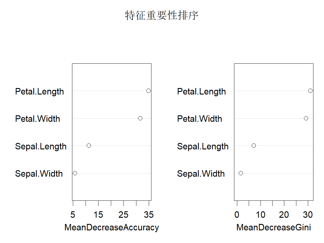

3、自动调参

target <- "Species" 

# 3. 自动调参网格：搜索 mtry + nodesize
# 范围可根据数据大小调整
mtry_seq <- 1:(ncol(train)-1)       # 特征数范围
nodesize_seq <- c(1,3,5,7,10)       # 叶子最小样本数

# 存储最优结果
best_oob <- Inf
best_param <- data.frame(mtry=NA, nodesize=NA)

cat("正在自动调参，请稍候...\n")

# 4. 双层循环自动搜索最优参数
for(mtry_val in mtry_seq){
  for(ns_val in nodesize_seq){
    
    set.seed(123)
    model <- randomForest(
      x = train[, !names(train) %in% target],  # 自变量
      y = factor(train[[target]]),            # 因变量
      ntree = 500,
      mtry = mtry_val,
      nodesize = ns_val,
      importance = TRUE
    )
    
    # OOB误差，模型真实性能，越小越好
    current_oob <- model$err.rate[nrow(model$err.rate), "OOB"]
    
    # 更新最优参数
    if(current_oob < best_oob){
      best_oob <- current_oob
      best_param <- data.frame(mtry=mtry_val, nodesize=ns_val)
    }
  }
}

# 5. 输出最优参数
cat("\n===== 最优参数结果 =====\n")
print(best_param)
cat("最优 OOB 误差：", round(best_oob,4), "\n")

最优 OOB 误差： 0.0381 

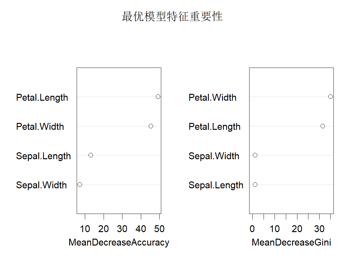
# 6. 使用最优参数训练最终模型
cat("\n正在训练最优模型...\n")
set.seed(123)
rf_final <- randomForest(
  x = train[, !names(train) %in% target],
  y = factor(train[[target]]),
  ntree = 1000,          # 最优模型多几棵树更稳
  mtry = best_param$mtry,
  nodesize = best_param$nodesize,
  importance = TRUE
)

# 7. 测试集评估
pred <- predict(rf_final, test)
acc <- mean(pred == test[[target]])
cat("\n测试集准确率：", round(acc,4), "\n")

测试集准确率： 0.9778 

4、保存模型

# 9.保存模型到本地文件
saveRDS(rf_final, file = "随机森林最优模型.rds")

# 10.加载模型
loaded_model <- readRDS("随机森林最优模型.rds")

# 11.用训练好的模型进行预测
pred <- predict(loaded_model, test)