【无标题】

2401_88566519

384人浏览 · 2026-05-19 20:01:40

2401_88566519 · 2026-05-19 20:01:40 发布

基于逻辑回归的银行贷款全流程实战

前言

在数字金融高速发展的今天，信用卡欺诈已成为全球银行与支付机构面临的核心风险之一。据相关行业统计，每年因信用卡欺诈造成的经济损失高达数百亿美元，且欺诈手段日趋智能化、隐蔽化，传统基于规则引擎的风控系统已难以应对复杂多变的欺诈模式。

信用卡欺诈检测本质上是一个二分类任务，但它具备两个极具挑战性的特点：

样本极度不平衡：正常交易占比超过99.7%，欺诈交易不足0.3%；
误判代价极不对称：漏判欺诈（FN）会直接造成资金损失，误判正常交易（FP）会影响用户体验。

因此，在欺诈检测场景中，准确率毫无意义，我们更关注少数类（欺诈）的召回率、精确率与F1值。

本文以经典Kaggle信用卡交易数据集为基础，从零开始实现一套完整的逻辑回归欺诈检测流程，内容涵盖：

逻辑回归数学原理与公式推导
Sklearn逻辑回归参数深度解析
数据预处理、标准化、EDA可视化
样本不平衡问题分析与处理思路
模型训练、交叉验证、超参数搜索
混淆矩阵、分类报告、阈值优化
完整可运行代码+详细注释

一、逻辑回归核心原理精讲

1.1 什么是逻辑回归

逻辑回归（Logistic Regression）名为回归，实为分类，是统计学与机器学习中最经典、最常用的线性二分类模型，广泛应用于金融风控、疾病预测、广告点击率预估等场景。

它的核心思想非常简洁：
在线性回归的输出基础上，套一层Sigmoid函数，将任意实数映射到(0,1)区间，从而将输出解释为样本属于正类的概率。

1.2 从线性回归到逻辑回归

线性回归模型：
$\theta_0 + \theta_1 x_1 + \theta_2 x_2 + \dots + \theta_n x_n = \boldsymbol{\theta}^T \boldsymbol{x}$

线性回归的问题：

输出范围为(-∞,+∞)，无法表示概率；
无法直接用于分类任务。

为了解决这个问题，逻辑回归引入Sigmoid函数。

1.3 Sigmoid函数详解

Sigmoid函数（Logistic函数）公式：
$\sigma(z) = \frac{1}{1 + e^{-z}}$

函数特点：

定义域：(-∞, +∞)
值域：(0, 1)
当 z=0 时，σ(z)=0.5
单调递增、无限平滑、可导

在这里插入图片描述

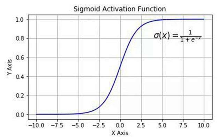
它的作用：
将线性回归的连续输出压缩成概率值，使模型输出具备真实的概率意义。

逻辑回归最终预测概率：
$\mid x;\theta) = \sigma(\boldsymbol{\theta}^T \boldsymbol{x}) = \frac{1}{1 + e^{-\boldsymbol{\theta}^T \boldsymbol{x}}}$

决策规则（默认阈值0.5）：
$y^={1,P≥0.50,P<0.5 \hat{y}= \begin{cases} 1, & P \ge 0.5 \\ 0, & P < 0.5 \end{cases}$

1.4 损失函数与极大似然估计

逻辑回归使用交叉熵损失（Cross Entropy Loss），而非均方误差。

单个样本损失：
$Loss(y^,y)=−[ylog⁡y^+(1−y)log⁡(1−y^)] Loss(\hat{y}, y) = -[y \log \hat{y} + (1-y) \log (1-\hat{y})]$

全局损失函数：
$J(\theta) = -\frac{1}{m} \sum_{i=1}^m \left[ y^{(i)} \log h_\theta(x^{(i)}) + (1-y^{(i)}) \log (1-h_\theta(x^{(i)})) \right]$

模型训练目标：最小化损失函数，通过梯度下降求解最优参数θ。

1.5 梯度下降公式推导

损失函数对参数θ_j求偏导：
$\frac{\partial J(\theta)}{\partial \theta_j} = \frac{1}{m} \sum_{i=1}^m \left( h_\theta(x^{(i)}) - y^{(i)} \right) x_j^{(i)}$

参数更新规则：
$\theta_j := \theta_j - \alpha \cdot \frac{1}{m} \sum_{i=1}^m \left( h_\theta(x^{(i)}) - y^{(i)} \right) x_j^{(i)}$

其中α为学习率。

二、Sklearn LogisticRegression 参数全解

LogisticRegression(
    penalty='l2',
    dual=False,
    tol=0.0001,
    C=1.0,
    fit_intercept=True,
    intercept_scaling=1,
    class_weight=None,
    random_state=None,
    solver='liblinear',
    max_iter=100,
    multi_class='auto',
    verbose=0,
    warm_start=False,
    n_jobs=None,
    l1_ratio=None
)

逻辑回归参数整理

2.1 正则化相关（防过拟合）

2.1.1 penalty
正则化类型：l1/l2
l1：服从拉普拉斯分布，可实现特征筛选
l2：服从高斯分布，通用性最强
注：newton-cg、sag、lbfgs仅支持L2正则

2.1.2 C
正则化强度系数，数值越小正则约束越强，抑制过拟合效果越好
默认值1.0，仅支持正浮点数

2.1.3 tol
迭代收敛判定精度，默认1e-4，达到设定精度即终止迭代训练

2.2 模型结构（截距/常数项）

2.2.1 fit_intercept
是否为模型添加截距项b，默认开启True，日常建模推荐启用

2.2.2 intercept_scaling
仅在选用liblinear求解器且开启截距项时生效，默认取值1.0

2.3 样本不平衡/分类权重

2.3.1 class_weight
用于平衡类别差异、调整错分损失

None：默认模式，不设置类别权重
balanced：依据样本数量自动分配权重，样本量越少权重越高
自定义字典：手动设定各类别权重占比

2.4 优化求解算法（solver）

2.4.1 liblinear（默认）
坐标轴下降法，适配小数据集、二分类场景

2.4.2 newton-cg
经典牛顿法，依托二阶导数运算，迭代次数少，运算开销大

2.4.3 lbfgs
拟牛顿法，适配高维特征数据，多用于多分类任务

2.4.4 sag
随机平均梯度下降法，专门适配海量样本数据集

2.4.5 saga
sag算法升级版本，兼容L1正则，适配大数据+高维特征场景

2.5 其余辅助参数

2.5.1 dual
对偶求解模式，默认关闭；样本数量大于特征数量时固定设为False

2.5.2 random_state
随机数种子，仅在sag、liblinear算法下生效，固定实验随机结果-

三、项目环境与数据集说明

3.1 开发环境

Python 3.11
Pandas、Numpy
Matplotlib
Scikit-learn
Jupyter Notebook

3.2 数据集介绍

数据集来源：Kaggle信用卡欺诈数据集

总行数：284807
特征数：30（V1-V28为PCA脱敏特征、Time、Amount）
标签：Class（0=正常，1=欺诈）
欺诈样本：492条，占比0.172%

数据已脱敏，无法看到原始交易信息，适合直接建模。

四、数据预处理全流程

4.1 读取数据

import pandas as pd
# 读取数据（出现编码/引擎报错可添加 encoding='utf8'、engine='python'）
data = pd.read_csv("./creditcard.csv")
# 查看前5行
print(data.head())

4.2 数据脱敏说明

数据脱敏是指对敏感信息进行加密、变形、替换等处理，在不破坏数据结构与分布的前提下，保护用户隐私。本数据中V1-V28均为脱敏特征。

4.3 特征标准化（Z-Score）

Amount数值范围极大，必须标准化，保证特征权重公平。

Z标准化公式：
$\frac{x - \mu}{\sigma}$

代码实现：

from sklearn.preprocessing import StandardScaler
scaler = StandardScaler()
data['Amount'] = scaler.fit_transform(data[['Amount']])

4.4 删除无用特征

data = data.drop(['Time'], axis=1)

4.5 样本分布可视化

import matplotlib.pyplot as plt
from pylab import mpl
# 解决matplotlib中文显示
mpl.rcParams['font.sans-serif'] = ['Microsoft YaHei']
mpl.rcParams['axes.unicode_minus'] = False

# 统计正负样本数量
labels_count = data['Class'].value_counts()
print("样本分布：\n", labels_count)

# 绘制柱状图
plt.title("正负例样本数")
plt.xlabel("类别")
plt.ylabel("频数")
labels_count.plot(kind='bar')
plt.show()

在这里插入图片描述

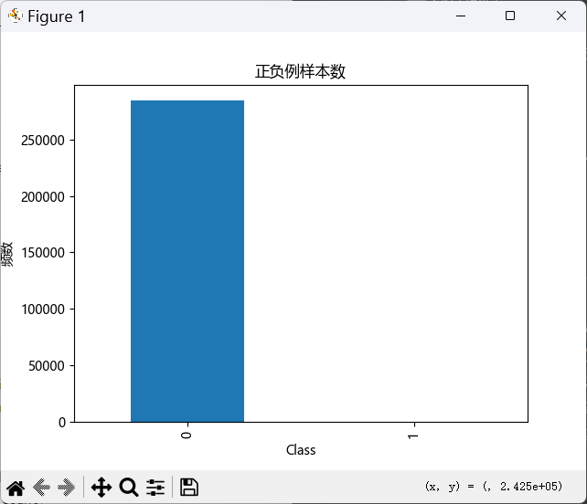
可以清晰看到：正常样本数量碾压欺诈样本。

五、数据集划分

from sklearn.model_selection import train_test_split

# 特征与标签分离
X = data.drop('Class', axis=1)
y = data.Class

# 训练集:测试集 = 7:3，固定随机种子保证可复现
x_train, x_test, y_train, y_test = train_test_split(
    X, y, test_size=0.3, random_state=1000
)

test_size=0.3：测试集占30%
random_state=1000：固定随机种子，保证可复现

六、基础模型训练（未调参）

from sklearn.linear_model import LogisticRegression
from sklearn import metrics

# 初始化逻辑回归（C=0.001 正则化强度）
lr = LogisticRegression(C=0.001, max_iter=1000)
# 模型训练
lr.fit(x_train, y_train)

# 训练集/测试集预测
train_predicted = lr.predict(x_train)
test_predicted = lr.predict(x_test)

# 分类报告（精确率、召回率、F1）
print("训练集分类报告：")
print(metrics.classification_report(y_train, train_predicted))
print("测试集分类报告：")
print(metrics.classification_report(y_test, test_predicted))

问题：样本不平衡导致欺诈类召回率极低，模型完全偏向多数类。

七、模型优化：交叉验证选最优C

逻辑回归中 C 是正则化强度倒数：C越小，正则化越强，防止过拟合。
使用8折交叉验证，以recall为指标选择最优C。

from sklearn.model_selection import cross_val_score
import numpy as np

# 候选C参数
c_param_range = [0.01, 0.1, 1, 10, 100]
scores = []

# 遍历C参数，交叉验证
for i in c_param_range:
    lr = LogisticRegression(C=i, penalty='l2', solver='lbfgs', max_iter=1000)
    # 8折交叉验证，指标为召回率recall
    score = cross_val_score(lr, x_train, y_train, cv=8, scoring='recall')
    score_mean = np.mean(score)
    scores.append(score_mean)
    print(f"C={i}，平均召回率：{score_mean:.4f}")

# 找到最优C
best_c = c_param_range[np.argmax(scores)]
print(f"\n===== 最优惩罚因子 C = {best_c} =====")

八、最优模型训练与评估

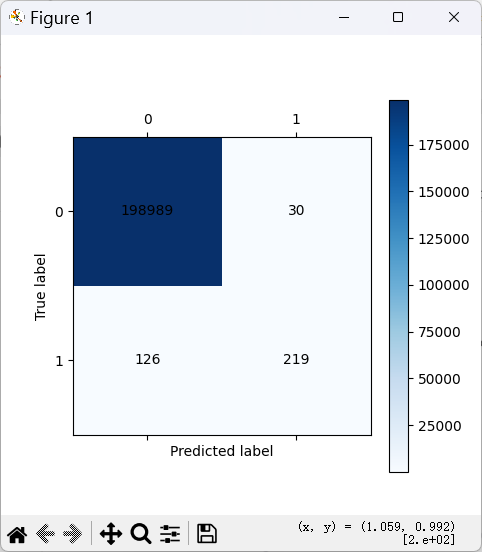
8.1 混淆矩阵可视化函数

def cm_plot(y, yp):
    """混淆矩阵可视化"""
    cm = metrics.confusion_matrix(y, yp)
    plt.matshow(cm, cmap=plt.cm.Blues)
    plt.colorbar()
    # 标注数值
    for x in range(len(cm)):
        for y in range(len(cm)):
            plt.annotate(cm[x, y], xy=(y, x), 
                         horizontalalignment='center',
                         verticalalignment='center')
    plt.ylabel('真实标签')
    plt.xlabel('预测标签')
    return plt

在这里插入图片描述

8.2 训练最优模型

# 使用最优C训练
lr_best = LogisticRegression(C=best_c, penalty='l2', max_iter=1000)
lr_best.fit(x_train, y_train)

# 训练集评估
train_pred = lr_best.predict(x_train)
print("训练集分类报告：")
print(metrics.classification_report(y_train, train_pred, digits=6))
cm_plot(y_train, train_pred).show()

# 测试集评估
test_pred = lr_best.predict(x_test)
print("测试集分类报告：")
print(metrics.classification_report(y_test, test_pred, digits=6))
cm_plot(y_test, test_pred).show()

九、进阶优化：调整分类阈值

逻辑回归默认阈值为0.5，对不平衡数据不友好。
遍历阈值[0.1,0.2,...,0.9]，找到召回率最优的阈值。

thresholds = [0.1, 0.2, 0.3, 0.4, 0.5, 0.6, 0.7, 0.8, 0.9]
recalls = []

for i in thresholds:
    # 预测概率
    y_pred_proba = lr_best.predict_proba(x_test)
    y_pred_proba = pd.DataFrame(y_pred_proba)
    # 只保留欺诈类概率
    y_pred_proba = y_pred_proba.drop([0], axis=1)
    # 自定义阈值
    y_pred_proba[y_pred_proba[1] > i] = 1
    y_pred_proba[y_pred_proba[1] <= i] = 0
    # 计算召回率
    recall = metrics.recall_score(y_test, y_pred_proba[1])
    recalls.append(recall)
    print(f"阈值={i}，测试集召回率：{recall:.3f}")

结论：降低阈值可显著提升欺诈样本召回率，业务中可根据风控要求取舍。

十、完整代码汇总

# ==================== 1. 导入库 ====================
import pandas as pd
import numpy as np
import matplotlib.pyplot as plt
from pylab import mpl
from sklearn.preprocessing import StandardScaler
from sklearn.model_selection import train_test_split, cross_val_score
from sklearn.linear_model import LogisticRegression
from sklearn import metrics

# ==================== 2. 中文设置 ====================
mpl.rcParams['font.sans-serif'] = ['Microsoft YaHei']
mpl.rcParams['axes.unicode_minus'] = False

# ==================== 3. 数据预处理 ====================
# 读取数据
data = pd.read_csv("./creditcard.csv")
print(data.head())

# Z标准化Amount
scaler = StandardScaler()
data['Amount'] = scaler.fit_transform(data[['Amount']])

# 删除无用列Time
data = data.drop(['Time'], axis=1)

# 样本分布可视化
labels_count = data['Class'].value_counts()
print("样本分布：\n", labels_count)
plt.title("正负例样本数")
plt.xlabel("类别")
plt.ylabel("频数")
labels_count.plot(kind='bar')
plt.show()

# ==================== 4. 数据集划分 ====================
X = data.drop('Class', axis=1)
y = data.Class
x_train, x_test, y_train, y_test = train_test_split(
    X, y, test_size=0.3, random_state=1000
)

# ==================== 5. 交叉验证选最优C ====================
c_param_range = [0.01, 0.1, 1, 10, 100]
scores = []
for i in c_param_range:
    lr = LogisticRegression(C=i, penalty='l2', solver='lbfgs', max_iter=1000)
    score = cross_val_score(lr, x_train, y_train, cv=8, scoring='recall')
    score_mean = np.mean(score)
    scores.append(score_mean)
    print(f"C={i}，平均召回率：{score_mean:.4f}")

best_c = c_param_range[np.argmax(scores)]
print(f"\n===== 最优惩罚因子 C = {best_c} =====")

# ==================== 6. 混淆矩阵函数 ====================
def cm_plot(y, yp):
    cm = metrics.confusion_matrix(y, yp)
    plt.matshow(cm, cmap=plt.cm.Blues)
    plt.colorbar()
    for x in range(len(cm)):
        for y in range(len(cm)):
            plt.annotate(cm[x, y], xy=(y, x), 
                         horizontalalignment='center',
                         verticalalignment='center')
    plt.ylabel('真实标签')
    plt.xlabel('预测标签')
    return plt

# ==================== 7. 最优模型训练与评估 ====================
lr_best = LogisticRegression(C=best_c, penalty='l2', max_iter=1000)
lr_best.fit(x_train, y_train)

# 训练集
train_pred = lr_best.predict(x_train)
print("训练集分类报告：")
print(metrics.classification_report(y_train, train_pred, digits=6))
cm_plot(y_train, train_pred).show()

# 测试集
test_pred = lr_best.predict(x_test)
print("测试集分类报告：")
print(metrics.classification_report(y_test, test_pred, digits=6))
cm_plot(y_test, test_pred).show()

# ==================== 8. 阈值优化 ====================
thresholds = [0.1,0.2,0.3,0.4,0.5,0.6,0.7,0.8,0.9]
for i in thresholds:
    y_pred_proba = lr_best.predict_proba(x_test)
    y_pred_proba = pd.DataFrame(y_pred_proba).drop([0], axis=1)
    y_pred_proba[y_pred_proba[1] > i] = 1
    y_pred_proba[y_pred_proba[1] <= i] = 0
    recall = metrics.recall_score(y_test, y_pred_proba[1])
    print(f"阈值={i}，召回率={recall:.3f}")