使用自定义后端进行匹配

在对样本集进行匹配时，我们可能想要使用非标准的距离测量或更快的实现方式。默认行为是使用 scikit-learn 的 NearestNeighbors 对象，但这可以通过在初始化 Matching、PropensityMatching 或 MatchingTransformer 对象时使用 knn_backend 关键字参数进行覆盖。

在这个笔记本中，我们展示了如何使用我们在 causallib.contrib 模块中提供的基于 Faiss 的后端。这可以在完整的 Lalonde 数据集上带来 5 倍或更大的速度提升，如下所示。

我们也展示了如何使用自定义的距离函数，通过在距离度量级别上实现倾向得分的对数比来匹配。

使用 Faiss 与 sklearn 的匹配性能对比

为了观察速度提升，我们像在 Lalonde 笔记本中一样加载增强的 Lalonde 数据集。接下来的几个单元格与我们在那里所做的相同。

import pandas as pd
import numpy as np
columns = ["training",   # Treatment assignment indicator
           "age",        # Age of participant
           "education",  # Years of education
           "black",      # Indicate whether individual is black
           "hispanic",   # Indicate whether individual is hispanic
           "married",    # Indicate whether individual is married
           "no_degree",  # Indicate if individual has no high-school diploma
           "re74",       # Real earnings in 1974, prior to study participation
           "re75",       # Real earnings in 1975, prior to study participation
           "re78"]       # Real earnings in 1978, after study end

#treated = pd.read_csv("http://www.nber.org/~rdehejia/data/nswre74_treated.txt", 
#                      delim_whitespace=True, header=None, names=columns)
#control = pd.read_csv("http://www.nber.org/~rdehejia/data/nswre74_control.txt",
#                      delim_whitespace=True, header=None, names=columns)
file_names = ["http://www.nber.org/~rdehejia/data/nswre74_treated.txt",
              "http://www.nber.org/~rdehejia/data/nswre74_control.txt",
              "http://www.nber.org/~rdehejia/data/psid_controls.txt",
              "http://www.nber.org/~rdehejia/data/psid2_controls.txt",
              "http://www.nber.org/~rdehejia/data/psid3_controls.txt",
              "http://www.nber.org/~rdehejia/data/cps_controls.txt",
              "http://www.nber.org/~rdehejia/data/cps2_controls.txt",
              "http://www.nber.org/~rdehejia/data/cps3_controls.txt"]
files = [pd.read_csv(file_name, delim_whitespace=True, header=None, names=columns) for file_name in file_names]
lalonde = pd.concat(files, ignore_index=True)
lalonde = lalonde.sample(frac=1.0, random_state=42)  # Shuffle

print(lalonde.shape)
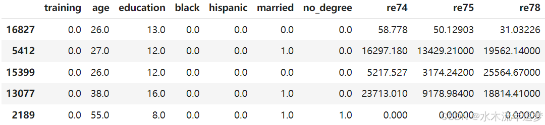
lalonde.head()
(22106, 10)

print(f'The dataset contains {lalonde.shape[0]} people, out of which {lalonde["training"].sum():.0f} received training')
The dataset contains 22106 people, out of which 185 received training
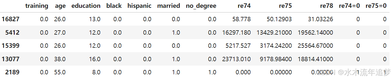
lalonde = lalonde.join((lalonde[["re74", "re75"]] == 0).astype(int), rsuffix=("=0"))
lalonde.head()

a = lalonde.pop("training")
y = lalonde.pop("re78")
X = lalonde
X.shape, a.shape, y.shape
((22106, 10), (22106,), (22106,))

在 Lalonde 匹配笔记本中，我们之前看到完整的 Lalonde 数据集进行匹配时相当慢。如果使用 contrib 模块中的 Faiss 后端，可以大幅度加快速度。如果可用，它将使用 GPU 加速，否则将回退到 CPU。下面的时间是在仅使用 CPU (Intel i7-9750H) 的情况下生成的。使用此后端需要安装来自 PyPI 的 faiss-gpu 或 faiss-cpu 包。

from causallib.estimation import Matching
from causallib.contrib.faissknn import FaissNearestNeighbors

sklearn 后端没有针对速度进行优化，大约需要 2 分钟来完成匹配。

⚠️警告⚠️：%%timeit 块可能需要很长时间来执行，因为它们运行多个试验。如果你出于除比较后端速度以外的目的运行此笔记本，你可能需要注释掉下面单元格的第一行。

%%timeit -n 2 -r 3 
m = Matching(knn_backend="sklearn")
m.fit(X,a,y)
y_potential_outcomes = m.estimate_population_outcome(X,a)
1min 51s ± 13.2 s per loop (mean ± std. dev. of 3 runs, 2 loops each)

knn_backend 参数可以是一个返回类似于 NearestNeighbors 对象的可调用对象或直接是一个对象。如果它是一个对象，那么该对象将被复制并对数据中的每个处理值进行拟合。这里我们使用类名作为可调用对象：

%%timeit -n 2 -r 3 
m = Matching(knn_backend=FaissNearestNeighbors)
m.fit(X,a,y)
y_potential_outcomes = m.estimate_population_outcome(X,a)
20.3 s ± 1.51 s per loop (mean ± std. dev. of 3 runs, 2 loops each)

这里我们使用 FaissNearestNeighbors 类的一个实例。有关支持的选项，请参阅 FaissNearestNeighbors 的文档。

%%timeit -n 2 -r 3 
m = Matching(knn_backend=FaissNearestNeighbors(index_type="ivfflat"))
m.fit(X,a,y)
y_potential_outcomes = m.estimate_population_outcome(X,a)
18.3 s ± 97.2 ms per loop (mean ± std. dev. of 3 runs, 2 loops each)

自定义距离函数：倾向得分的对数比

在使用倾向得分比较两个样本之间的差异时，原始差值可能是误导性的。这是因为 0.01 和 0.05 之间的差异远比 0.51 和 0.55 之间的差异更有意义。在《统计学、社会科学和生物医学科学的因果推断》一书的第 18.5 节中，Imbens 和 Rubin 建议采用“对数比”
$$l(x)=ln(x/(1-x))$$
并在该尺度上比较倾向得分的差异。这不是 Matching 的默认行为，但很容易实现。

def logodds(x):
    return np.log( x / (1 - x))
def logodds_distance(x,y):
    return np.abs(logodds(x) - logodds(y))
def check_difference(x,y):
    print("({x:.2f},{y:.2f}): original distance: {d1:.2f} logodds distance: {d2:.2f}"
          .format_map({"x":x,"y":y,"d1":np.abs(x-y),"d2":logodds_distance(x,y)}))
check_difference(0.01,0.05)
check_difference(0.51,0.55)
(0.01,0.05): original distance: 0.04 logodds distance: 1.65
(0.51,0.55): original distance: 0.04 logodds distance: 0.16

这对于匹配是有用的，因为倾向为 0.51 的样本与倾向为 0.55 的样本相匹配可能比倾向为 0.01 的样本与倾向为 0.05 的样本相匹配更好。

我们通过将 logodds_distance 函数传递给 NearestNeighbors 并将其作为 PropensityMatching 的 knn_backend 来实现这一点。

from causallib.estimation import PropensityMatching
from sklearn.neighbors import NearestNeighbors
from sklearn.linear_model import LogisticRegression

logodds_knn = NearestNeighbors(metric=logodds_distance)

为了便于速度比较，我们将加载 causallib 提供的 NHEFS 数据。

from causallib.datasets import load_nhefs

data_nhefs = load_nhefs(augment=False,onehot=False)
X_nhefs, a_nhefs, y_nhefs = data_nhefs.X, data_nhefs.a, data_nhefs.y

我们可以使用倾向得分匹配和对数比距离来估计总体结果，其中倾向模型是逻辑回归。

pm_nhefs_log = PropensityMatching(
    learner=LogisticRegression(solver="liblinear"),
    knn_backend=logodds_knn,
    ).fit(X_nhefs, a_nhefs, y_nhefs)
pm_nhefs_log.estimate_population_outcome(X_nhefs, a_nhefs)
0    1.802614
1    4.560399
dtype: float64

为了比较，我们使用标准的欧几里得度量来拟合相同的数据。

pm_nhefs_lin = PropensityMatching(
    learner=LogisticRegression(solver="liblinear"),
    knn_backend="sklearn"
    ).fit(X_nhefs,a_nhefs,y_nhefs)
pm_nhefs_lin.estimate_population_outcome(X_nhefs,a_nhefs)
0    1.802614
1    4.548021
dtype: float64

我们可以类似地使用对数比来进行完整的 Lalonde 数据集的匹配，并使用卡尺来解决 Lalonde 匹配笔记本中讨论的不平衡问题：

pm_lalonde_log = PropensityMatching(
    learner=LogisticRegression(solver="liblinear"),
    knn_backend=logodds_knn,
    caliper=0.01,
    ).fit(X, a, y)
pm_lalonde_log.estimate_population_outcome(X, a)
0.0    6340.629027
1.0    7201.100363
dtype: float64

FaissNearestNeighbors 对象目前不支持除了马哈拉诺比斯和欧几里得之外的其他度量。

注意：在实践中，可以表达为对协变量变换的替代度量（如对数比）应该放在倾向转换对象中，而不是放在度量函数中。这将大幅加速运行时间，因为自定义函数比内置的 NearestNeighbors 度量更慢，并且不被 FaissNearestNeighbors 后端支持。