1. class VectorValues

This class represents a collection of vector-valued variables associated each with a unique integer index. It is typically used to store the variables of a GaussianFactorGraph.

Optimizing a GaussianFactorGraph or GaussianBayesNet returns this class.

For basic usage, such as receiving a linear solution from gtsam solving functions, or creating this class in unit tests and examples where speed is not important, you can use a simple interface:

• The default constructor VectorValues() to create this class

• insert (Key, const Vector&) to add vector variables

• operator for read and write access to stored variables

• \ref exists (Key) to check if a variable is present

• Other facilities like iterators, size(), dim(), etc.

Example:

VectorValues values;

values.emplace(3, Vector3(1.0, 2.0, 3.0));

values.emplace(4, Vector2(4.0, 5.0));

values.emplace(0, (Vector(4) << 6.0, 7.0, 8.0, 9.0).finished());

// Prints [ 3.0 4.0 ]

gtsam::print(values[1]);

// Prints [ 8.0 9.0 ]

values[1] = Vector2(8.0, 9.0);

gtsam::print(values[1]);

2. struct SlotEntry

One SlotEntry stores the slot index for a variable, as well its dim

3. class Scatter

class Scatter : public FastVector<SlotEntry>

Scatter is an intermediate data structure used when building a HessianFactor incrementally, to get the keys in the right order. In spirit, it is a map from global variable indices to slot indices in the union of involved variables. We also include the dimensionality of the variable.

主要用于存储SlotEntry，用于保存生个变量的维度

Scatter(const GaussianFactorGraph& gfg, const Ordering& ordering)

gfg中所有相关的key都建立一个槽（SlotEntry），但是在ordering中的key放在前面，不在其中的放在后面

注意：最后对在ordering中的key进行了一个排序，令人费解

4. class Ordering

4.1. class Ordering: public KeyVector

主要用于对节点进行排序，它继承了KeyVector，每一个Key对应一个节点，根据这些Key就对节点进行排序了。

4.2. Ordering ColamdConstrained(const VariableIndex& variableIndex, const FastMap<Key, int>& groups)

Compute a fill-reducing ordering using constrained COLAMD from a VariableIndex. In this function, a group for each variable should be specified in \c groups, and each group of variables will appear in the ordering in group index order. \c groups should be a map from Key to group index. The group indices used should be consecutive starting at 0, but may appear in \c groups in arbitrary order. Any variables not present in \c groups will be assigned to group 0. This function simply fills the \c cmember argument to CCOLAMD with the supplied indices, see the CCOLAMD documentation for more information.

经过测试，输出按groups排序，即所有group为0的排最前面，group 1的次之，以此类推。输出的Key与输入的Key是保持一致的，没有删减。

4.2. Ordering ColamdConstrained(const VariableIndex& variableIndex, std::vector<int>& cmember)

真正干活的函数

5. class VerticalBlockMatrix

This class stores a dense matrix and allows it to be accessed as a collection of vertical blocks. The dimensions of the blocks are provided when constructing this class.

This class also has three parameters that can be changed after construction that change the apparent view of the matrix without any reallocation or data copying. firstBlock() determines the block that has index 0 for all operations (except for re-setting firstBlock()). rowStart() determines the apparent first row of the matrix for all operations (except for setting rowStart() and rowEnd()). rowEnd() determines the apparent exclusive (one-past-the-last) last row for all operations. To include all rows, rowEnd() should be set to the number of rows in the matrix (i.e. one after the last true row index).

竖条状的块矩阵，可以用于保存增广矩阵，即雅克比矩阵的增广矩阵，这样左侧每一列对应一个变量，最右侧对应b值

LikeActiveViewOf(const SymmetricBlockMatrix& rhs, DenseIndex height)

Copy the block structure, but do not copy the matrix data. If blockStart() has been modified, this copies the structure of the corresponding matrix view. In the destination

VerticalBlockMatrix, blockStart() will be 0.

6. class SymmetricBlockMatrix

This class stores a dense matrix and allows it to be accessed as a collection of blocks. When constructed, the caller must provide the dimensions of the blocks. The block structure is symmetric, but the underlying matrix does not necessarily need to be. This class also has a parameter that can be changed after construction to change the apparent matrix view. firstBlock() determines the block that appears to have index 0 for all operations(except re-setting firstBlock()).

该类用于表示分块矩阵，因为是对称矩阵，所以是方阵。该类可以根据块索引来获取对应的矩阵块。

从该类的使用上来看，好像只有右上角是填值的，左下角完全留空，它的意思可能是：这是对称矩阵，所以只需要填右上角，左下角就是右上角的转置，所以无需填充。

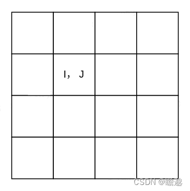
6.1. updateDiagonalBlock(DenseIndex I, const XprType& xpr)

把xpr矩阵的右上角加到对应的对角块上去，注意只使用右上角，且是加上去，而非赋值

6.2. updateOffDiagonalBlock(DenseIndex I, DenseIndex J, const XprType& xpr)

把xpr加到非对角块上去，注意是加上去，而非赋值

如果索引的是右上角的块，则直接加；如果索引的左下角的块，则把xpr的转置加到相应的右上角

6.3. choleskyPartial(DenseIndex nFrontals)

7. class GaussianFactor

class GTSAM_EXPORT GaussianFactor : public Factor

An abstract virtual base class for JacobianFactor and HessianFactor. A GaussianFactor has a quadratic error function. GaussianFactor is non-mutable (all methods const!). The factor value is

$$exp(-0.5*||Ax-b||^2)$$

7.1. Matrix augmentedJacobian()

Return a dense $$[ \;A\;b\; ] \in \mathbb{R}^{m \times n+1}$$Jacobian matrix, augmented with b with the noise models baked into A and b. The negative log-likelihood is $$\frac{1}{2} \Vert Ax-b \Vert^2$$.

See also GaussianFactorGraph::jacobian and GaussianFactorGraph::sparseJacobian.

7.2. std::pair<Matrix,Vector> jacobian()

Return the dense Jacobian A and right-hand-side b, with the noise models baked into A and b. The negative log-likelihood is $$\frac{1}{2} \Vert Ax-b \Vert^2$$.

See also GaussianFactorGraph::augmentedJacobian and GaussianFactorGraph::sparseJacobian.

7.3. Matrix augmentedInformation()

Return the augmented information matrix represented by this GaussianFactor. The augmented information matrix contains the information matrix with an additional column holding the information vector, and an additional row holding the transpose of the information vector. The lower-right entry contains the constant error term (when $$\delta x = 0$$). The augmented information matrix is described in more detail in HessianFactor, which in fact stores an augmented information matrix.

8. class GaussianFactorGraph

class GaussianFactorGraph : public FactorGraph<GaussianFactor>, public EliminateableFactorGraph<GaussianFactorGraph>

A Linear Factor Graph is a factor graph where all factors are Gaussian, i.e.

Factor == GaussianFactor

VectorValues = A values structure of vectors

Most of the time, linear factor graphs arise by linearizing a non-linear factor graph.

9. Class Conditional

Base class for conditional densities, templated on KEY type. This class provides storage for the keys involved in a conditional, and iterators and access to the frontal and separator keys.

Derived classes *must* redefine the Factor and shared_ptr typedefs to refer to the associated factor type and shared_ptr type of the derived class. See IndexConditional and GaussianConditional for examples.

10. class GaussianConditional

class GaussianConditional : public JacobianFactor, public Conditional<JacobianFactor, GaussianConditional>

A conditional Gaussian functions as the node in a Bayes network It has a set of parents y, z, etc. and implements a probability density on x.

The negative log-probability is given by$$\frac{1}{2} |Rx - (d - Sy - Tz - ...)|^2$$

注意区分nrFrontals()和front()

nrFrontals()继承于Conditional，返回的是贝叶斯树的front的个数

front()继承于JacobianFactor，最终继承于Factor，

10.1. shared_ptr Combine(ITERATOR firstConditional, ITERATOR lastConditional)

Combine several GaussianConditional into a single dense GC. The conditionals enumerated by \c first and \c last must be in increasing order, meaning that the parents of any conditional may not include a conditional coming before it.

param firstConditional Iterator to the first conditional to combine, must dereference to a shared_ptr<GaussianConditional>.

param lastConditional Iterator to after the last conditional to combine, must dereference to a shared_ptr<GaussianConditional>.

10.2. VectorValues solve(const VectorValues& parents)

Solves a conditional Gaussian and writes the solution into the entries of x for each frontal variable of the conditional. The parents are assumed to have already been solved in and their values are read from x.

This function works for multiple frontal variables.

Given the Gaussian conditional with log likelihood$$|R x_f - (d - S x_s)|^2$$, where f are the frontal variables and s are the separator variables of this conditional, this solve function computes$$x_f = R^{-1} (d - S x_s)$$using back-substitution.

param parents VectorValues containing solved parents$$x_s$$.

11. class JacobianFactor

class JacobianFactor : public GaussianFactor

A Gaussian factor in the squared-error form.

JacobianFactor implements a Gaussian, which has quadratic negative log-likelihood$$E(x) = \frac{1}{2} (Ax-b)^T \Sigma^{-1} (Ax-b)$$

where$$\Sigma $$is a diagonal covariance matrix. The matrix A, r.h.s. vector b, and diagonal noise model

This factor represents the sum-of-squares error of a linear measurement function, and is created upon linearization of a NoiseModelFactor, which in turn is a sum-of-squares factor with a nonlinear measurement function.

Here is an example of how this factor represents a sum-of-squares error

Letting h(x) be a linear measurement prediction function, z be the actual observed measurement, the residual is$$f(x) = h(x) - z$$.If we expect noise with diagonal covariance matrix$$\Sigma$$on this measurement, then the negative log-likelihood of the Gaussian induced by this measurement model is

$$E(x) = \frac{1}{2} (h(x) - z)^T \Sigma^{-1} (h(x) - z)$$Because h(x) is linear, we can write it as h(x) = Ax + e and thus we have$$E(x) = \frac{1}{2} (Ax-b)^T \Sigma^{-1} (Ax-b)$$where b = z - e.

This factor can involve an arbitrary number of variables, and in the above example x would almost always be only be a subset of the variables in the entire factor graph. There are special constructors for 1-, 2-, and 3-way JacobianFactors, and additional constructors for creating n-way JacobianFactors.

The Jacobian matrix A is passed to these constructors in blocks, for example, for a 2-way factor, the constructor would accept A1 and A2, as well as the variable indices j1 and j2 and the negative log-likelihood represented by this factor would be$$E(x) = \frac{1}{2} (A_1 x_{j1} + A_2 x_{j2} - b)^T \Sigma^{-1} (A_1 x_{j1} + A_2 x_{j2} - b) $$

updateHessian(const KeyVector& infoKeys, SymmetricBlockMatrix* info)

把该因子的jacobian矩阵更新到传入的hessian矩阵info中，需要仔细阅读一下该函数

12. class HessianFactor

class HessianFactor : public GaussianFactor

A Gaussian factor using the canonical parameters (information form)

HessianFactor implements a general quadratic factor of the form

$$E(x) = 0.5 x^T G x - x^T g + 0.5 f $$

that stores the matrix G, the vector g, and the constant term f. When G is positive semidefinite, this factor represents a Gaussian, in which case G is the information matrix$$\Lambda$$, g is the information vector$$\eta$$, and f is the residual sum-square-error at the mean, when$$x = \mu$$.Indeed, the negative log-likelihood of a Gaussian is (up to a constant)

$$E(x) = 0.5(x-\mu)^T P^{-1} (x-\mu)$$

with$$\mu$$the mean and P the covariance matrix. Expanding the product we get

$$E(x) = 0.5 x^T P^{-1} x - x^T P^{-1} \mu + 0.5 \mu^T P^{-1} \mu$$

We define the Information matrix (or Hessian)$$\Lambda = P^{-1}$$

and the information vector

$$\eta = P^{-1} \mu = \Lambda \mu$$

to arrive at the canonical form of the Gaussian:

$$E(x) = 0.5 x^T \Lambda x - x^T \eta + 0.5 \mu^T \Lambda \mu$$

This factor is one of the factors that can be in a GaussianFactorGraph. It may be returned from NonlinearFactor::linearize(), but is also used internally to store the Hessian during Cholesky elimination.

This can represent a quadratic factor with characteristics that cannot be represented using a JacobianFactor (which has the form$$E(x) = \Vert Ax - b \Vert^2$$and stores the Jacobian A and error vector b, i.e. is a sum-of-squares factor). For example, a HessianFactor need not be positive semidefinite, it can be indefinite or even negative semidefinite.

If a HessianFactor is indefinite or negative semi-definite, then in order for solving the linear system to be possible, the Hessian of the full system must be positive definite (i.e. when all small Hessians are combined, the result must be positive definite). If this is not the case, an error will occur during elimination.

This class stores G, g, and f as an augmented matrix HessianFactor::matrix_. The upper-left n x n blocks of HessianFactor::matrix_ store the upper-right triangle of G, the upper-right-most column of length n of HessianFactor::matrix_ stores g, and the lower-right entry of HessianFactor::matrix_ stores f, i.e.

HessianFactor::matrix_ = [ G11 G12 G13 ... g1

0 G22 G23 ... g2

0 0 G33 ... g3

: : : :

0 0 0 ... f ]

Blocks can be accessed as follows:

G11 = info(begin(), begin());

G12 = info(begin(), begin()+1);

G23 = info(begin()+1, begin()+2);

g2 = linearTerm(begin()+1);

f = constantTerm();

.......

12.1. HessianFactor(const GaussianFactorGraph& factors, const Scatter& scatter)

先调用Allocate为info_分配内存，然后每个因子的hessian矩阵放到info_的对应位置

12.2. EliminateCholesky(const GaussianFactorGraph& factors, const Ordering& keys)

先用构造HessianFactor，然后该HessianFactor做eliminateCholesky消元，消元的结果是conditional

把conditional和HessianFactor组成pair一起返回

12.3. Allocate(const Scatter& scatter)

主要是分配内存，把变量key依次放入成员变量keys_中，同时按变量的维度给成员变量块矩阵info_分配内存

12.4. updateHessian(const KeyVector& infoKeys, SymmetricBlockMatrix* info)

把该因子的info_的块加到info的对应块中。info_的块是按key来划分的，infoKeys有几个key就分别按行和列划分，它在info中的索引由infoKeys来决定，这里面key的顺序决定这个索引。

12.5. _FromJacobianHelper

由雅克比矩阵生成海森矩阵

13. Eigen::TriangularView< _MatrixType, _Mode >

This class represents a triangular part of a matrix, not necessarily square. Strictly speaking, for rectangular matrices one should speak of "trapezoid" parts. This class is the return type of MatrixBase::triangularView() and SparseMatrixBase::triangularView(), and most of the time this is the only way it is used.

14. class noiseModel::Base

noiseModel::Base is the abstract base class for all noise models.

Noise models must implement a 'whiten' function to normalize an error vector, and an 'unwhiten' function to unnormalize an error vector.

15. class noiseModel::Gaussian

Gaussian implements the mathematical model$$|Rx|^2 = |y|^2$$with$$R'R=inv(Sigma)$$where

y = whiten(x) = Rx, x = unwhiten(x) = inv(R)y as indeed$$|y|^2 = y'y = x'R'Rx$$Various derived classes are available that are more efficient.

the underlying object might be a derived class such as Diagonal.

16. class NoiseModelFactor

class NoiseModelFactor: public NonlinearFactor

A nonlinear sum-of-squares factor with a zero-mean noise model implementing the density$$P(z|x) \propto exp -0.5*|z-h(x)|^2_C$$

Templated on the parameter type X and the values structure Values

There is no return type specified for h(x). Instead, we require the derived class implements $$\mathtt{error\_vector}(x) = h(x)-z \approx A \delta x - b$$

This allows a graph to have factors with measurements of mixed type.

The noise model is typically Gaussian, but robust and constrained error models are also supported.

17. EliminateableFactorGraph

EliminateableFactorGraph is a base class for factor graphs that contains elimination algorithms. Any factor graph holding eliminateable factors can derive from this class to expose functions for computing marginals, conditional marginals, doing multifrontal and sequential elimination, etc.

18. Cholesky

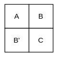
18.1. choleskyPartial(Matrix& ABC, size_t nFrontal, size_t topleft)

topleft是ABC左上角的起始点，nFrontal是A的尺寸

Unable to copy while content loads

对A进行LLT分解，

19. treeTraversal-inst.h

DepthFirstForest

Traverse a forest depth-first with pre-order and post-order visits.

EliminatableClusterTree forest: The forest of trees to traverse. The method forest.roots() should exist and return a collection of (shared) pointers to FOREST::Node.

EliminationData rootData: The data to pass by reference to visitorPre when it is called on each root node.

visitorPre: visitorPre(node, parentData) will be called at every node, before visiting its children, and will be passed, by reference, the DATA object returned by the visit to its parent. Likewise, visitorPre should return the DATA object to pass to the children. The returned DATA object will be copy-constructed only upon returning to store internally, thus may be modified by visiting the children. Regarding efficiency, this copy-on-return is usually optimized out by the compiler.

visitorPost visitorPost(node, data) will be called at every node, after visiting its children, and will be passed, by reference, the DATA object returned by the call to visitorPre (the DATA object may be modified by visiting the children).

重要函数，按照深度优先的方式实现了变量消元

• forest.roots_中的元素全部构造TraversalNode类对象并入栈，给它们一个共同的父节点rootData
• 访问栈顶的TraversalNode类对象，直到栈为空时退出
• 如果是第一次处理该对象，先用它构造EliminationData类对象并插入到dataList中，再把TraversalNode类对象的dataPointer指向EliminationData类对象
• 把TraversalNode类对象的所有孩子构造TraversalNode类对象并入栈，同时保证TraversalNode类对象仍然是它们的父节点
• 如果之前已经处理过该对象，调用visitorPost函数处理该对象并把它弹出栈

20. class JunctionTree

class JunctionTree : public EliminatableClusterTree<BAYESTREE, GRAPH>

A JunctionTree is a cluster tree, a set of variable clusters with factors, arranged in a tree,

with the additional property that it represents the clique tree associated with a Bayes Net.

In GTSAM a junction tree is an intermediate data structure in multifrontal variable

elimination. Each node is a cluster of factors, along with a clique of variables that are

eliminated all at once. In detail, every node k represents a clique (maximal fully connected

subset) of an associated chordal graph, such as a chordal Bayes net resulting from elimination.

The difference with the BayesTree is that a JunctionTree stores factors, whereas a

BayesTree stores conditionals, that are the product of eliminating the factors in the

corresponding JunctionTree cliques.

The tree structure and elimination method are exactly analagous to the EliminationTree,

except that in the JunctionTree, at each node multiple variables are eliminated at a time.

21. EliminationTree

这是一个非常重要的类

An elimination tree is a data structure used intermediately during elimination. In future versions it will be used to save work between multiple eliminations.

When a variable is eliminated, a new factor is created by combining that variable's neighboring factors. The new combined factor involves the combined factors' involved variables.

When the lowest-ordered one of those variables is eliminated, it consumes that combined factor. In the elimination tree, that lowest-ordered variable is the parent of the variable that was eliminated to

produce the combined factor.

This yields a tree in general, and not a chain because of the implicit sparse structure of the resulting Bayes net.

This structure is examined even more closely in a JunctionTree, which additionally identifies cliques in the chordal Bayes net.

21.1. EliminationTree(const FactorGraphType& graph, const VariableIndex& structure, const Ordering& order)

If we already hit a variable in this factor, make the subtree containing the previous variable in this factor a child of the current node. This means that the variables eliminated earlier in the factor depend on the later variables in the factor. If we haven't yet hit a variable in this factor, we add the factor to the current node.

这里只是建立消元树，并未进行真正意义上的消元，建立消元树是为了给接下来的消元做准备。

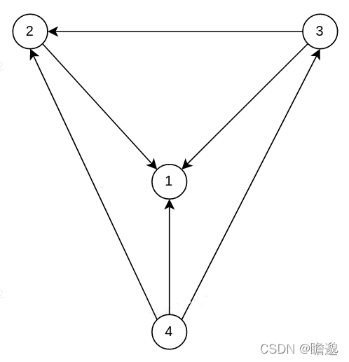
变量消元过程中，后来居上，后来的是父节点，先来的是子节点。子节点的子节点也自己的子节点。

如下图所示，数字表示顺序，箭头表示父子关系。图中以较为复杂的四元因子为例，实际多为一元因子或二元因子。

函数在运行过程中把因子分配到成员变量是roots_中（注意这是消元数的成员变量，与贝叶斯树的成员变量roots_不同），剩下一些因子存放到remainingFactors_中。为什么会有剩余的因子？

21.2. std::pair<boost::shared_ptr<BAYESNET>, boost::shared_ptr<GRAPH>> EliminationTree<BAYESNET,GRAPH>::eliminate(Eliminate function)

主要调用inference-inst.h中的eliminate函数

22. class GaussianEliminationTree

GaussianEliminationTree(const GaussianFactorGraph& factorGraph, const VariableIndex& structure, const Ordering& order);

*Build the elimination tree of a factor graph using pre-computed column structure.

@param factorGraph The factor graph for which to build the elimination tree

@param structure The set of factors involving each variable. If this is not precomputed, you can call the Create(const FactorGraph<DERIVEDFACTOR>&) named constructor instead.

@return The elimination tree

23. inference-inst.h

FastVector<typename TREE::sharedFactor> EliminateTree(RESULT& result, const TREE& tree, const typename TREE::Eliminate& function)

struct EliminationPostOrderVisitor

24. Class VariableIndex

The VariableIndex class computes and stores the block column structure of a factor graph. The factor graph stores a collection of factors, each of which involves a set of variables. In contrast, the VariableIndex is built from a factor graph prior to elimination, and stores the list of factors that involve each variable. This information is stored as a deque of lists of factor indices.

看名字好像是一个很简单的类，其实它同时管理了key和factor index，保存每一个key对应的所有factor index

24.1. void augment(const FG& factors, boost::optional<const FactorIndices&> newFactorIndices = boost::none)

Augment the variable index with new factors. This can be used when solving problems incrementally.

24.2. void augmentExistingFactor(const FactorIndex factorIndex, const KeySet & newKeys)

Augment the variable index after an existing factor now affects to more variable Keys. This can be used when solving problems incrementally, with smart factors or in general with factors with a dynamic number of Keys.

25. ClusterTree.h

25.1. struct Cluster

A Cluster is just a collection of factors

FastVector<boost::shared_ptr<Cluster>> children; // sub-trees

Ordering orderedFrontalKeys; // Frontal keys of this node

FactorGraphType factors; // Factors associated with this node

25.2. class ClusterTree

A cluster-tree is associated with a factor graph and is defined as in Koller-Friedman: each node k represents a subset $$C_k \sub X$$, and the tree is family preserving, in that each factor f_i is associated with a single cluster and $$ scope(f_i) \sub C_k$$

比较简单的一个类，主要维护了成员变量roots_

25.3. EliminatableClusterTree

std::pair<boost::shared_ptr<BayesTreeType>, boost::shared_ptr<FactorGraphType>>

eliminate(const Eliminate& function) const;

主要的函数，实现了因子图的消元，生成贝叶斯树

26. ClusterTree-inst.h

26.1. Struct EliminationData

EliminationData构造函数

EliminationPreOrderVisitor(const EliminatableClusterTree::sharedNode& node, EliminationData& parentData)

构造了一个EliminationData类对象并返回

26.2. Class EliminationData::EliminationPostOrderVisitor

operator()

27. class BayesTree

27.1. nodes_

Nodes类型的成员变量，Nodes本质上是键值映射表，键和值分别为Key和sharedClique，类似于std::map<Key, sharedClique>，用于记录每个key对应的团

每个key只与一个sharedClique相关联吗？注意，这里的值是sharedClique，而非factor。如果只看spliter或者frontal，一个key确实只与一个sharedClique相关。至于这里的对应关系是key->spliter还是key->frontal，还有待确定

27.2. roots_

Roots类型的成员变量，本质上是std::vector<sharedClique>，但它只保存根节点

27.3. removeTop(const KeyVector& keys, BayesNetType* bn, Cliques* orphans)

把这些节点及其父节点的conditional_放入贝叶斯网中，把它们的子节点放入orphans成为孤儿

27.4. saveGraph(const std::string& s, const KeyFormatter& keyFormatter = DefaultKeyFormatter)

saves the Tree to a text file in GraphViz format

27.5. removeSubtree(const sharedClique& subtree)

• 如果subtree是根，则直接从roots_中删除；否则从其父节的子节点列表中删除
• 依次记录subtree及所有的后代节点
• 让这些节点的缓存清空，断绝与父节点的关系，清空子节点列表
• 把这些节点的frontals()中的key从nodes_中删除，注意这里调用了unsafe_erase函数，是不安全的
• 把所有被删除的sharedClique收集起来作为返回值

28. BayesTreeCliqueBase

This is the base class for BayesTree cliques. The default and standard derived type is BayesTreeClique, but some algorithms, like iSAM2, use a different clique type in order to store extra data along with the clique.

This class is templated on the derived class (i.e. the curiously recursive template pattern). The advantage of this over using virtual classes is that it avoids the need for casting to get the derived type. This is possible because all cliques in a BayesTree are the same type - if they were not then we'd need a virtual class.

shortcut

separatorMarginal

29. ISAM2Clique

注意一下这个成员变量，与边缘化有关

Base::FactorType::shared_ptr cachedFactor_;

它来自源于HessianFactor::EliminatePreferCholesky函数中调用的EliminateQR或EliminateCholesky函数返回值的second