本文摘要：正则化是防止机器学习模型过拟合的关键技术。过拟合指模型死记硬背训练数据而无法泛化，表现为训练误差极低但测试误差很高。正则化通过给模型"戴上枷锁"来限制复杂度，主要分为L1（Lasso）和L2（Ridge）两种方法：L2使所有参数缩小但不为零，L1会将不重要参数变为零实现特征选择。通过多项式回归和房价预测案例演示了正则化的实际应用，并强调需用交叉验证选择最佳正则化参数。最终建议：识别过拟合后，根据需求选择正则化方法（Ridge防过拟合、Lasso做特征选择），使用自动调参工具优化参数，并在测试集验证性能。

---

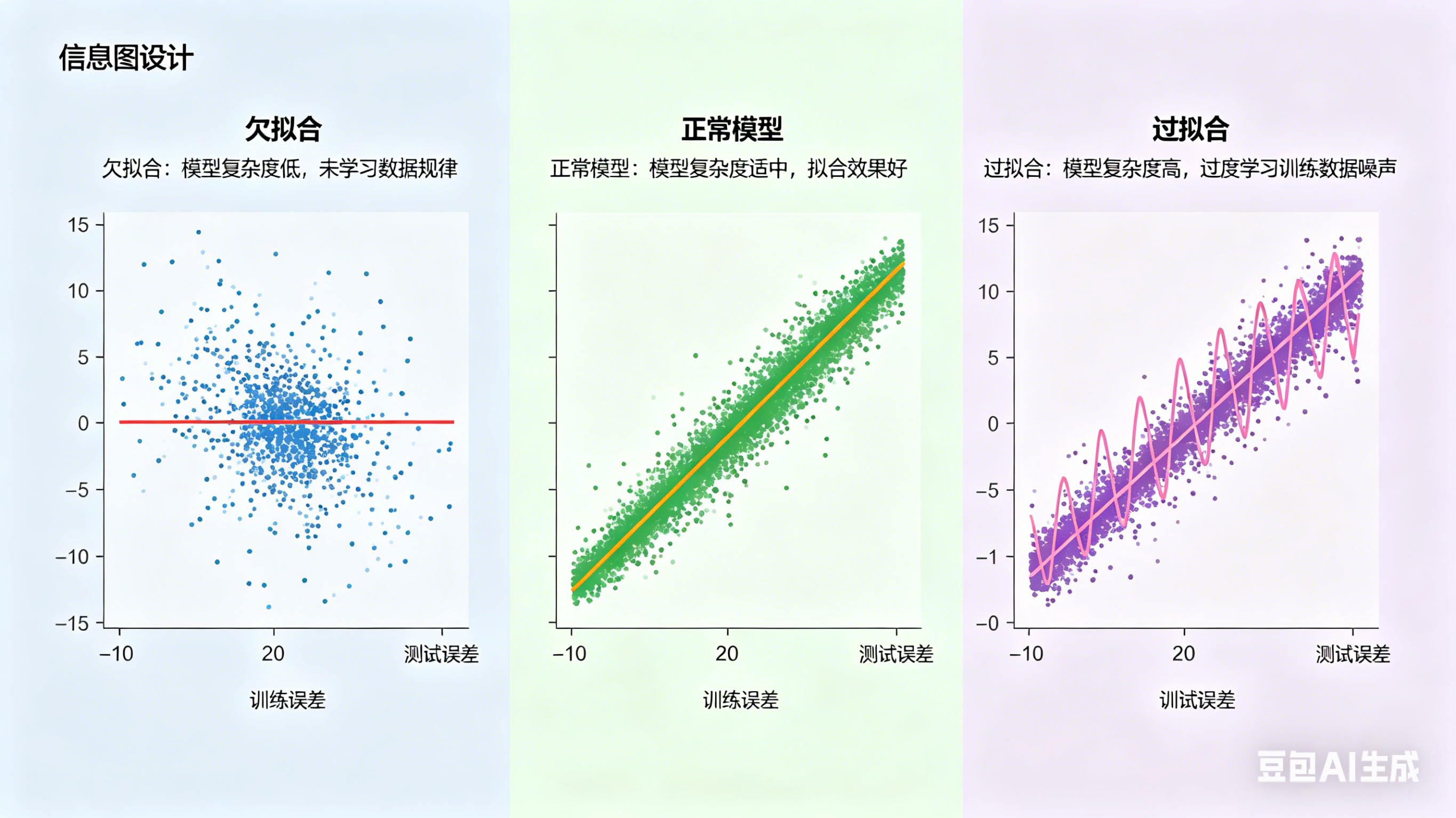
1. 人话解释

1.1 什么是过拟合？

text

想象你在准备考试：

┌─────────────────────────────────────────────────────────┐
│ 学渣的学习方式（欠拟合）                                  │
├─────────────────────────────────────────────────────────┤
│  • 只记住"加法就是把数字加起来"                          │
│  • 考试：1+1=? → 能答对 ✓                               │
│  • 考试：123+456=? → 不会 ✗                             │
│  • 问题：学得太粗糙，连基本规律都没掌握                  │
└─────────────────────────────────────────────────────────┘

┌─────────────────────────────────────────────────────────┐
│ 好学生的学习方式（恰当拟合）                              │
├─────────────────────────────────────────────────────────┤
│  • 理解加法的原理和规律                                  │
│  • 练习题：1+1=2, 2+3=5 → 理解规律                      │
│  • 考试：任何加法题 → 都能做对 ✓                        │
│  • 关键：掌握了通用规律，能应对新题目                    │
└─────────────────────────────────────────────────────────┘

┌─────────────────────────────────────────────────────────┐
│ 死记硬背的学习方式（过拟合）                              │
├─────────────────────────────────────────────────────────┤
│  • 把练习题的答案全背下来                                │
│  • 练习题：1+1=2 → 100%正确 ✓                           │
│  • 练习题：2+3=5 → 100%正确 ✓                           │
│  • 考试：1+1=? → 答对（背过）✓                          │
│  • 考试：3+4=? → 不会（没背过）✗                        │
│  • 问题：只记住了答案，没理解规律                        │
└─────────────────────────────────────────────────────────┘

过拟合的本质：模型"背答案"而不是"学规律"

Python

# 用代码直观展示
import numpy as np
import matplotlib.pyplot as plt

# 真实规律：y = sin(x)
X = np.array([0, 1, 2, 3, 4, 5, 6])  # 7个训练点
y = np.sin(X) + np.random.normal(0, 0.1, len(X))  # 加噪声

# 过拟合模型：用6次多项式强行通过所有点
from sklearn.preprocessing import PolynomialFeatures
from sklearn.linear_model import LinearRegression

poly = PolynomialFeatures(degree=6)
X_poly = poly.fit_transform(X.reshape(-1, 1))
model = LinearRegression()
model.fit(X_poly, y)

# 绘制
X_plot = np.linspace(-1, 7, 200)
X_plot_poly = poly.transform(X_plot.reshape(-1, 1))
y_plot = model.predict(X_plot_poly)

plt.figure(figsize=(12, 5))

plt.subplot(1, 2, 1)
plt.scatter(X, y, s=100, c='red', zorder=3, edgecolors='black', linewidth=2)
plt.plot(X_plot, y_plot, 'b-', linewidth=2)
plt.plot(X_plot, np.sin(X_plot), 'g--', linewidth=2, alpha=0.5)
plt.title('过拟合：完美通过训练点，但曲线乱飞', fontsize=14, fontweight='bold')
plt.xlabel('X')
plt.ylabel('Y')
plt.legend(['过拟合模型', '真实规律', '训练数据'])
plt.grid(True, alpha=0.3)

# 在新数据上的表现
X_new = np.array([0.5, 1.5, 2.5, 3.5, 4.5, 5.5])
y_new_true = np.sin(X_new)
X_new_poly = poly.transform(X_new.reshape(-1, 1))
y_new_pred = model.predict(X_new_poly)

plt.subplot(1, 2, 2)
plt.scatter(X_new, y_new_true, s=100, c='green', label='真实值', zorder=3, edgecolors='black', linewidth=2)
plt.scatter(X_new, y_new_pred, s=100, c='red', marker='x', s=200, label='预测值', linewidth=3)
for i in range(len(X_new)):
    plt.plot([X_new[i], X_new[i]], [y_new_true[i], y_new_pred[i]], 'k--', alpha=0.5)
plt.title('在新数据上：预测严重偏离真实值', fontsize=14, fontweight='bold', color='red')
plt.xlabel('X')
plt.ylabel('Y')
plt.legend()
plt.grid(True, alpha=0.3)

plt.tight_layout()
plt.savefig('overfitting_intuition.png', dpi=100)
plt.show()

print("=" * 70)
print("过拟合演示")
print("=" * 70)
print(f"训练数据上的误差: {np.mean((y - model.predict(X_poly))**2):.6f} (非常小)")
print(f"新数据上的误差: {np.mean((y_new_true - y_new_pred)**2):.6f} (非常大)")
print("\n这就是过拟合：训练误差很小，但测试误差很大！")
print("=" * 70)

1.2 什么是正则化？

text

正则化 = 给模型"戴上枷锁"，防止它"死记硬背"

┌─────────────────────────────────────────────────────────┐
│ 没有正则化                                               │
├─────────────────────────────────────────────────────────┤
│  模型：我要用尽全力拟合每一个训练点！                    │
│  结果：训练误差 = 0.0001（完美！）                       │
│       测试误差 = 10.5（糟糕！）                         │
│  问题：过拟合                                            │
└─────────────────────────────────────────────────────────┘

┌─────────────────────────────────────────────────────────┐
│ 使用正则化                                               │
├─────────────────────────────────────────────────────────┤
│  我们：等等！不要太复杂，简单一点！                      │
│  模型：好吧，我稍微放松一点...                           │
│  结果：训练误差 = 0.05（稍微差一点）                     │
│       测试误差 = 0.08（好多了！）                       │
│  效果：泛化能力提升                                      │
└─────────────────────────────────────────────────────────┘

正则化的三个比喻：

text

比喻1：画画比赛
  无正则化：用100种颜色，画得极其复杂，但只适合这一张纸
  有正则化：只用10种颜色，画得简洁，适用于各种纸张

比喻2：写作文
  无正则化：用尽所有华丽辞藻，堆砌成复杂长句
  有正则化：用简单直白的语言，表达清晰

比喻3：编程
  无正则化：写1000行复杂代码，处理每个特殊情况
  有正则化：写100行简洁代码，遵循通用规律

1.3 两种正则化方法

text

┌─────────────────────────────────────────────────────────────┐
│ L2 正则化 (Ridge) - 让所有参数都变小                         │
├─────────────────────────────────────────────────────────────┤
│                                                             │
│  原始参数: [100, 0.5, -80, 0.3, 120, -0.1]                 │
│           ↓ 正则化后                                        │
│  新参数:   [10,  0.4, -8,  0.2, 12,  -0.08]                │
│                                                             │
│  效果：所有参数都缩小，但都保留                              │
│  比喻：把音量都调小，但不关掉任何声道                        │
│                                                             │
└─────────────────────────────────────────────────────────────┘

┌─────────────────────────────────────────────────────────────┐
│ L1 正则化 (Lasso) - 把不重要的参数变成0                      │
├─────────────────────────────────────────────────────────────┤
│                                                             │
│  原始参数: [100, 0.5, -80, 0.3, 120, -0.1]                 │
│           ↓ 正则化后                                        │
│  新参数:   [50,  0,   -40,  0,   60,   0]                  │
│                                                             │
│  效果：小的参数变为0，只保留重要的                           │
│  比喻：关掉不重要的声道，只保留主要的                        │
│  应用：特征选择（自动识别重要特征）                          │
│                                                             │
└─────────────────────────────────────────────────────────────┘

视觉对比：

Python

import numpy as np
import matplotlib.pyplot as plt
from sklearn.linear_model import Ridge, Lasso

# 生成数据
np.random.seed(42)
n_features = 20
X = np.random.randn(100, n_features)
# 只有前5个特征有用，后15个是噪声
true_coef = np.array([5, -3, 2, -1, 1] + [0]*15)
y = X @ true_coef + np.random.randn(100) * 0.5

# 训练三个模型
from sklearn.linear_model import LinearRegression

model_lr = LinearRegression().fit(X, y)
model_ridge = Ridge(alpha=1.0).fit(X, y)
model_lasso = Lasso(alpha=0.1).fit(X, y)

# 可视化系数
fig, axes = plt.subplots(1, 4, figsize=(16, 4))

# 真实系数
axes[0].bar(range(n_features), true_coef, color='green', alpha=0.7, edgecolor='black')
axes[0].set_title('真实系数\n(只有前5个有用)', fontsize=12, fontweight='bold')
axes[0].set_xlabel('特征编号')
axes[0].set_ylabel('系数值')
axes[0].axhline(y=0, color='red', linestyle='--', linewidth=1)
axes[0].grid(True, alpha=0.3, axis='y')

# 无正则化
axes[1].bar(range(n_features), model_lr.coef_, color='red', alpha=0.7, edgecolor='black')
axes[1].set_title('无正则化\n(所有系数都很大，包括噪声)', fontsize=12, fontweight='bold', color='red')
axes[1].set_xlabel('特征编号')
axes[1].set_ylabel('系数值')
axes[1].axhline(y=0, color='red', linestyle='--', linewidth=1)
axes[1].grid(True, alpha=0.3, axis='y')

# Ridge
axes[2].bar(range(n_features), model_ridge.coef_, color='blue', alpha=0.7, edgecolor='black')
axes[2].set_title('Ridge (L2)\n(所有系数都缩小)', fontsize=12, fontweight='bold', color='blue')
axes[2].set_xlabel('特征编号')
axes[2].set_ylabel('系数值')
axes[2].axhline(y=0, color='red', linestyle='--', linewidth=1)
axes[2].grid(True, alpha=0.3, axis='y')

# Lasso
axes[3].bar(range(n_features), model_lasso.coef_, color='purple', alpha=0.7, edgecolor='black')
axes[3].set_title('Lasso (L1)\n(噪声特征变为0)', fontsize=12, fontweight='bold', color='purple')
axes[3].set_xlabel('特征编号')
axes[3].set_ylabel('系数值')
axes[3].axhline(y=0, color='red', linestyle='--', linewidth=1)
axes[3].grid(True, alpha=0.3, axis='y')

plt.tight_layout()
plt.savefig('regularization_comparison.png', dpi=100)
plt.show()

# 统计非零系数
print("=" * 70)
print("系数对比")
print("=" * 70)
print(f"真实模型: {np.sum(true_coef != 0)} 个非零系数")
print(f"无正则化: {np.sum(np.abs(model_lr.coef_) > 0.01)} 个非零系数 (都很大)")
print(f"Ridge:    {np.sum(np.abs(model_ridge.coef_) > 0.01)} 个非零系数 (都缩小)")
print(f"Lasso:    {np.sum(np.abs(model_lasso.coef_) > 0.01)} 个非零系数 (自动选择)")
print("\n结论：Lasso 正确识别出了5个有用特征！")
print("=" * 70)

1.4 正则化参数 α (lambda)

text

α (正则化强度) 就像"刹车力度"

α = 0 (无刹车)
┌─────────────────────────────┐
│  模型：我要全速冲刺！        │
│  结果：冲太快，过拟合        │
│  训练误差：0.01             │
│  测试误差：10.5             │
└─────────────────────────────┘

α = 适中 (刚好的刹车)
┌─────────────────────────────┐
│  模型：我保持稳定速度        │
│  结果：刚刚好，泛化最佳      │
│  训练误差：0.5              │
│  测试误差：0.6              │
└─────────────────────────────┘

α = 很大 (刹车太猛)
┌─────────────────────────────┐
│  模型：我几乎停下来了...     │
│  结果：太保守，欠拟合        │
│  训练误差：5.0              │
│  测试误差：5.1              │
└─────────────────────────────┘

关键概念总结（人话版）：

概念	人话解释	记忆口诀
过拟合	死记硬背，不懂规律	训练完美，测试糟糕
欠拟合	太懒，连基本的都不学	训练测试都不好
正则化	限制模型不要太复杂	给模型戴枷锁
L1 (Lasso)	把不重要的扔掉	做减法，变稀疏
L2 (Ridge)	把所有都缩小	打折扣，变平滑
α 参数	控制限制的强度	刹车力度

2. 数学推导

2.1 线性回归的代价函数（回顾）

无正则化的代价函数：

J(θ)=12m∑i=1m(hθ(x(i))−y(i))2J(θ)=2m1​i=1∑m​(hθ​(x(i))−y(i))2

其中：

• mm = 样本数量
• hθ(x)=θ0+θ1x1+...+θnxn=θTxhθ​(x)=θ0​+θ1​x1​+...+θn​xn​=θTx
• 目标：min⁡θJ(θ)minθ​J(θ) （让误差最小）

问题：当特征很多或多项式阶数很高时，模型会学到很大的参数 θθ，导致过拟合。

text

例如：
  无正则化：y = 1 + 2x + 300x² - 500x³ + 800x⁴
           参数巨大，曲线剧烈波动
  
  理想状态：y = 1 + 2x + 0.1x²
           参数适中，曲线平滑

2.2 L2 正则化（Ridge Regression）

核心思想：在原始代价函数上加一个"惩罚项"，惩罚过大的参数。

代价函数：

J(θ)=12m∑i=1m(hθ(x(i))−y(i))2+λ2m∑j=1nθj2J(θ)=2m1​i=1∑m​(hθ​(x(i))−y(i))2+2mλ​j=1∑n​θj2​

拆解：

J(θ)=12m∑i=1m(hθ(x(i))−y(i))2⏟原始误差项（拟合好坏）+λ2m∑j=1nθj2⏟正则化项（惩罚复杂度）J(θ)=原始误差项（拟合好坏）2m1​i=1∑m​(hθ​(x(i))−y(i))2​​+正则化项（惩罚复杂度）2mλ​j=1∑n​θj2​​​

符号说明：

• λλ (lambda)：正则化参数（控制惩罚强度）
  • λ=0λ=0：无正则化
  • λλ 很大：强正则化
• ∑j=1nθj2∑j=1n​θj2​：所有参数的平方和（注意：不包括 θ0θ0​）

为什么是平方？

text

参数值      平方      效果
----------------------------------------
θ = 0       0²=0      不惩罚
θ = 1       1²=1      轻微惩罚
θ = 10      10²=100   重度惩罚
θ = 100     100²=10000 严重惩罚

结论：参数越大，惩罚越重（呈平方增长）

矩阵形式：

J(θ)=12m(Xθ−y)T(Xθ−y)+λ2mθTθJ(θ)=2m1​(Xθ−y)T(Xθ−y)+2mλ​θTθ

求解（正规方程）：

对 J(θ)J(θ) 求导并令其为0：

∇θJ(θ)=1mXT(Xθ−y)+λmθ=0∇θ​J(θ)=m1​XT(Xθ−y)+mλ​θ=0

整理得：

XTXθ+λθ=XTyXTXθ+λθ=XTy(XTX+λI)θ=XTy(XTX+λI)θ=XTy

最终解：

θ=(XTX+λI)−1XTyθ=(XTX+λI)−1XTy​

其中 II 是单位矩阵。

重要性质：

1. 当 λ=0λ=0 时，退化为普通线性回归
2. λIλI 使得矩阵始终可逆（解决了普通线性回归的奇异性问题）
3. 所有 θjθj​ 都会缩小，但不会变成0

梯度下降形式：

θj:=θj−α[1m∑i=1m(hθ(x(i))−y(i))xj(i)+λmθj]θj​:=θj​−α[m1​i=1∑m​(hθ​(x(i))−y(i))xj(i)​+mλ​θj​]

整理：

θj:=θj(1−αλm)−α1m∑i=1m(hθ(x(i))−y(i))xj(i)θj​:=θj​(1−αmλ​)−αm1​i=1∑m​(hθ​(x(i))−y(i))xj(i)​

解释：

• (1−αλm)(1−αmλ​)：这一项略小于1，每次迭代都会让 θjθj​ 稍微缩小
• 这就是为什么叫 "权重衰减"（Weight Decay）

2.3 L1 正则化（Lasso Regression）

代价函数：

J(θ)=12m∑i=1m(hθ(x(i))−y(i))2+λ2m∑j=1n∣θj∣J(θ)=2m1​i=1∑m​(hθ​(x(i))−y(i))2+2mλ​j=1∑n​∣θj​∣

与 L2 的区别：

项目	L2 (Ridge)	L1 (Lasso)
正则化项	∑θj2∑θj2​	∑∥θj∥∑∥θj​∥
几何意义	圆形约束	菱形约束
参数性质	缩小但不为0	可以变为0
解的形式	有闭式解	无闭式解（需要迭代）

为什么 L1 会产生稀疏解？

text

几何直觉：

L2 正则化（圆形约束）         L1 正则化（菱形约束）
        θ₂                          θ₂
        │                           │
        │    ⚪                      │    ◇
    ────┼────  θ₁               ────┼────  θ₁
        │                           │
        │                           │

等高线更可能在"平滑"处         等高线更可能在"尖角"处
相切，参数不为0                相切，参数变为0

数学解释：

L1 的次梯度（subgradient）：

∂∂θj∣θj∣={+1if θj>0[−1,1]if θj=0−1if θj<0∂θj​∂​∣θj​∣=⎩⎨⎧​+1[−1,1]−1​if θj​>0if θj​=0if θj​<0​

梯度下降更新：

θj:=θj−α[1m∑i=1m(hθ(x(i))−y(i))xj(i)+λmsign(θj)]θj​:=θj​−α[m1​i=1∑m​(hθ​(x(i))−y(i))xj(i)​+mλ​sign(θj​)]

其中 sign(θj)sign(θj​) 是符号函数：

sign(θj)={+1if θj>00if θj=0−1if θj<0sign(θj​)=⎩⎨⎧​+10−1​if θj​>0if θj​=0if θj​<0​

软阈值操作（Soft Thresholding）：

θj={θj−λmif θj>λm0if ∣θj∣≤λmθj+λmif θj<−λmθj​=⎩⎨⎧​θj​−mλ​0θj​+mλ​​if θj​>mλ​if ∣θj​∣≤mλ​if θj​<−mλ​​

这解释了为什么参数会变为0。

2.4 Elastic Net（结合 L1 和 L2）

代价函数：

J(θ)=12m∑i=1m(hθ(x(i))−y(i))2+λ(α∑j=1n∣θj∣+1−α2∑j=1nθj2)J(θ)=2m1​i=1∑m​(hθ​(x(i))−y(i))2+λ(αj=1∑n​∣θj​∣+21−α​j=1∑n​θj2​)

其中：

• λλ：总的正则化强度
• α∈[0,1]α∈[0,1]：L1 和 L2 的混合比例
  • α=0α=0：纯 L2 (Ridge)
  • α=1α=1：纯 L1 (Lasso)
  • α=0.5α=0.5：L1 和 L2 各占一半

优点：

• 结合了 L1 的特征选择能力
• 结合了 L2 的稳定性
• 当特征相关时，比纯 Lasso 更稳定

2.5 正则化参数 λ 的选择

交叉验证选择 λ：

text

算法流程：

1. 准备候选值：λ ∈ {0.001, 0.01, 0.1, 1, 10, 100}

2. For each λ:
     For each fold in K-fold:
         在训练折上训练模型
         在验证折上评估
     计算平均验证误差

3. 选择验证误差最小的 λ

数学表达：

λ∗=arg⁡min⁡λCV-Error(λ)λ∗=argλmin​CV-Error(λ)

其中：

CV-Error(λ)=1K∑k=1KErrork(λ)CV-Error(λ)=K1​k=1∑K​Errork​(λ)

正则化路径（Regularization Path）：

text

随着 λ 增大，参数的变化：

λ=0        λ=0.1      λ=1        λ=10       λ=100
θ₁: 100  →  50    →   10    →    1     →    0.01
θ₂:  80  →  40    →    8    →    0.8   →    0.008
θ₃: -60  → -30    →   -6    →   -0.6   →   -0.006
θ₄:   5  →   3    →    1    →    0.1   →    0.001

3. 完整案例

3.1 案例1：多项式回归中的过拟合与正则化

import numpy as np
import matplotlib.pyplot as plt
from sklearn.preprocessing import PolynomialFeatures
from sklearn.linear_model import LinearRegression, Ridge, Lasso
from sklearn.model_selection import train_test_split, cross_val_score
from sklearn.metrics import mean_squared_error, r2_score
from sklearn.pipeline import Pipeline
import warnings
warnings.filterwarnings('ignore')

print("=" * 80)
print("              案例1：多项式回归 - 过拟合与正则化完整演示")
print("=" * 80)

# ============================================================
# 步骤1：生成数据
# ============================================================
np.random.seed(42)

# 真实函数：y = sin(x) + 噪声
n_samples = 30
X = np.sort(np.random.uniform(0, 10, n_samples))
y_true = np.sin(X)
y = y_true + np.random.normal(0, 0.2, n_samples)

X_train = X.reshape(-1, 1)
y_train = y

# 测试数据（密集点，用于绘制平滑曲线）
X_plot = np.linspace(0, 10, 200).reshape(-1, 1)
y_plot_true = np.sin(X_plot.flatten())

print(f"\n数据集信息:")
print(f"  训练样本: {n_samples} 个点")
print(f"  真实函数: y = sin(x) + 噪声")
print(f"  噪声水平: σ = 0.2")

# ============================================================
# 步骤2：演示过拟合
# ============================================================
print("\n" + "=" * 80)
print("步骤2：对比不同复杂度的模型")
print("=" * 80)

degrees = [1, 3, 9, 15]
models = {}

fig, axes = plt.subplots(2, 2, figsize=(14, 10))
axes = axes.ravel()

for idx, degree in enumerate(degrees):
    # 训练模型（无正则化）
    poly = PolynomialFeatures(degree=degree)
    X_train_poly = poly.fit_transform(X_train)
    X_plot_poly = poly.transform(X_plot)
    
    model = LinearRegression()
    model.fit(X_train_poly, y_train)
    
    # 预测
    y_pred_train = model.predict(X_train_poly)
    y_pred_plot = model.predict(X_plot_poly)
    
    # 评估
    train_error = mean_squared_error(y_train, y_pred_train)
    
    # 保存结果
    models[degree] = {
        'model': model,
        'poly': poly,
        'train_error': train_error,
        'coef': model.coef_
    }
    
    # 可视化
    ax = axes[idx]
    ax.scatter(X_train, y_train, s=50, alpha=0.7, edgecolors='black', 
               linewidth=1, label='训练数据', zorder=3)
    ax.plot(X_plot, y_plot_true, 'g--', linewidth=2, alpha=0.7, 
            label='真实函数 sin(x)')
    ax.plot(X_plot, y_pred_plot, 'r-', linewidth=2.5, label=f'拟合 (degree={degree})')
    
    # 判断拟合状态
    if degree == 1:
        status = "欠拟合"
        color = 'orange'
    elif degree == 3:
        status = "恰当拟合"
        color = 'green'
    elif degree == 9:
        status = "开始过拟合"
        color = 'blue'
    else:
        status = "严重过拟合"
        color = 'red'
    
    ax.set_title(f'{status} (degree={degree})\n训练误差={train_error:.4f}',
                 fontweight='bold', fontsize=12, color=color)
    ax.set_xlabel('X')
    ax.set_ylabel('Y')
    ax.legend(loc='upper right')
    ax.grid(True, alpha=0.3)
    ax.set_ylim(-2, 2)

plt.tight_layout()
plt.savefig('overfitting_demo.png', dpi=100)
plt.show()

print(f"\n{'阶数':<8} {'训练误差':<15} {'参数数量':<12} {'最大参数':<12}")
print("-" * 55)
for degree in degrees:
    info = models[degree]
    print(f"{degree:<8} {info['train_error']:<15.4f} {len(info['coef']):<12} "
          f"{np.max(np.abs(info['coef'])):<12.2f}")

print("\n观察:")
print("  • degree=15 训练误差最小，但曲线剧烈波动（过拟合）")
print("  • 高阶模型的参数值非常大（最大参数 > 10^6）")
print("  • 这就需要正则化来控制参数大小")

# ============================================================
# 步骤3：应用正则化
# ============================================================
print("\n" + "=" * 80)
print("步骤3：使用正则化解决过拟合（degree=15）")
print("=" * 80)

degree_high = 15
poly_high = PolynomialFeatures(degree=degree_high)
X_train_poly_high = poly_high.fit_transform(X_train)
X_plot_poly_high = poly_high.transform(X_plot)

# 训练三个模型
# 1. 无正则化
model_none = LinearRegression()
model_none.fit(X_train_poly_high, y_train)

# 2. Ridge (L2)
model_ridge = Ridge(alpha=1.0)
model_ridge.fit(X_train_poly_high, y_train)

# 3. Lasso (L1)
model_lasso = Lasso(alpha=0.01, max_iter=10000)
model_lasso.fit(X_train_poly_high, y_train)

# 预测
y_pred_none = model_none.predict(X_plot_poly_high)
y_pred_ridge = model_ridge.predict(X_plot_poly_high)
y_pred_lasso = model_lasso.predict(X_plot_poly_high)

# 可视化对比
fig, axes = plt.subplots(2, 2, figsize=(14, 10))

# 图1：无正则化
ax1 = axes[0, 0]
ax1.scatter(X_train, y_train, s=50, alpha=0.7, edgecolors='black', linewidth=1)
ax1.plot(X_plot, y_plot_true, 'g--', linewidth=2, alpha=0.7, label='真实函数')
ax1.plot(X_plot, y_pred_none, 'r-', linewidth=2, label='无正则化')
ax1.set_title('无正则化 - 严重过拟合', fontweight='bold', color='red', fontsize=12)
ax1.legend()
ax1.grid(True, alpha=0.3)
ax1.set_ylim(-2, 2)

# 图2：Ridge
ax2 = axes[0, 1]
ax2.scatter(X_train, y_train, s=50, alpha=0.7, edgecolors='black', linewidth=1)
ax2.plot(X_plot, y_plot_true, 'g--', linewidth=2, alpha=0.7, label='真实函数')
ax2.plot(X_plot, y_pred_ridge, 'b-', linewidth=2, label='Ridge (L2)')
ax2.set_title('Ridge 正则化 - 平滑拟合', fontweight='bold', color='blue', fontsize=12)
ax2.legend()
ax2.grid(True, alpha=0.3)
ax2.set_ylim(-2, 2)

# 图3：Lasso
ax3 = axes[1, 0]
ax3.scatter(X_train, y_train, s=50, alpha=0.7, edgecolors='black', linewidth=1)
ax3.plot(X_plot, y_plot_true, 'g--', linewidth=2, alpha=0.7, label='真实函数')
ax3.plot(X_plot, y_pred_lasso, 'm-', linewidth=2, label='Lasso (L1)')
ax3.set_title('Lasso 正则化 - 稀疏解', fontweight='bold', color='purple', fontsize=12)
ax3.legend()
ax3.grid(True, alpha=0.3)
ax3.set_ylim(-2, 2)

# 图4：参数对比
ax4 = axes[1, 1]
n_features = len(model_none.coef_)
x_pos = np.arange(n_features)

width = 0.25
ax4.bar(x_pos - width, model_none.coef_, width, label='无正则化', 
        alpha=0.7, edgecolor='black')
ax4.bar(x_pos, model_ridge.coef_, width, label='Ridge', 
        alpha=0.7, edgecolor='black')
ax4.bar(x_pos + width, model_lasso.coef_, width, label='Lasso', 
        alpha=0.7, edgecolor='black')

ax4.set_xlabel('特征编号')
ax4.set_ylabel('系数值')
ax4.set_title('参数对比 (degree=15)', fontweight='bold', fontsize=12)
ax4.legend()
ax4.grid(True, alpha=0.3, axis='y')
ax4.axhline(y=0, color='red', linestyle='--', linewidth=1)

plt.tight_layout()
plt.savefig('regularization_effect.png', dpi=100)
plt.show()

# 统计信息
print(f"\n{'方法':<15} {'训练MSE':<12} {'非零系数':<12} {'最大参数':<12}")
print("-" * 55)

coef_none_nonzero = np.sum(np.abs(model_none.coef_) > 1e-6)
coef_ridge_nonzero = np.sum(np.abs(model_ridge.coef_) > 1e-6)
coef_lasso_nonzero = np.sum(np.abs(model_lasso.coef_) > 1e-6)

mse_none = mean_squared_error(y_train, model_none.predict(X_train_poly_high))
mse_ridge = mean_squared_error(y_train, model_ridge.predict(X_train_poly_high))
mse_lasso = mean_squared_error(y_train, model_lasso.predict(X_train_poly_high))

print(f"{'无正则化':<15} {mse_none:<12.4f} {coef_none_nonzero:<12} "
      f"{np.max(np.abs(model_none.coef_)):<12.2e}")
print(f"{'Ridge (L2)':<15} {mse_ridge:<12.4f} {coef_ridge_nonzero:<12} "
      f"{np.max(np.abs(model_ridge.coef_)):<12.2f}")
print(f"{'Lasso (L1)':<15} {mse_lasso:<12.4f} {coef_lasso_nonzero:<12} "
      f"{np.max(np.abs(model_lasso.coef_)):<12.2f}")

print("\n关键发现:")
print("  ✓ Ridge: 所有系数都缩小，曲线变平滑")
print("  ✓ Lasso: 很多系数变为0，自动特征选择")
print("  ✓ 两者训练误差略高，但泛化能力更强")

# ============================================================
# 步骤4：选择最佳正则化参数 α
# ============================================================
print("\n" + "=" * 80)
print("步骤4：交叉验证选择最佳正则化参数")
print("=" * 80)

# 准备候选参数
alphas = np.logspace(-3, 3, 50)  # 0.001 到 1000

# 使用交叉验证
from sklearn.model_selection import cross_val_score

ridge_scores = []
lasso_scores = []

for alpha in alphas:
    # Ridge
    pipe_ridge = Pipeline([
        ('poly', PolynomialFeatures(degree=15)),
        ('ridge', Ridge(alpha=alpha))
    ])
    score_ridge = -cross_val_score(pipe_ridge, X_train, y_train, 
                                    cv=5, scoring='neg_mean_squared_error').mean()
    ridge_scores.append(score_ridge)
    
    # Lasso
    pipe_lasso = Pipeline([
        ('poly', PolynomialFeatures(degree=15)),
        ('lasso', Lasso(alpha=alpha, max_iter=10000))
    ])
    score_lasso = -cross_val_score(pipe_lasso, X_train, y_train, 
                                    cv=5, scoring='neg_mean_squared_error').mean()
    lasso_scores.append(score_lasso)

# 找到最佳参数
best_alpha_ridge = alphas[np.argmin(ridge_scores)]
best_alpha_lasso = alphas[np.argmin(lasso_scores)]

# 可视化
plt.figure(figsize=(12, 5))

plt.subplot(1, 2, 1)
plt.semilogx(alphas, ridge_scores, 'b-', linewidth=2, label='Ridge')
plt.axvline(x=best_alpha_ridge, color='red', linestyle='--', linewidth=2,
            label=f'最佳 α = {best_alpha_ridge:.3f}')
plt.xlabel('正则化参数 α', fontsize=12)
plt.ylabel('交叉验证 MSE', fontsize=12)
plt.title('Ridge: 选择最佳正则化参数', fontsize=14, fontweight='bold')
plt.legend()
plt.grid(True, alpha=0.3)

plt.subplot(1, 2, 2)
plt.semilogx(alphas, lasso_scores, 'm-', linewidth=2, label='Lasso')
plt.axvline(x=best_alpha_lasso, color='red', linestyle='--', linewidth=2,
            label=f'最佳 α = {best_alpha_lasso:.3f}')
plt.xlabel('正则化参数 α', fontsize=12)
plt.ylabel('交叉验证 MSE', fontsize=12)
plt.title('Lasso: 选择最佳正则化参数', fontsize=14, fontweight='bold')
plt.legend()
plt.grid(True, alpha=0.3)

plt.tight_layout()
plt.savefig('alpha_selection.png', dpi=100)
plt.show()

print(f"\n最佳参数:")
print(f"  Ridge: α = {best_alpha_ridge:.4f}, CV-MSE = {min(ridge_scores):.4f}")
print(f"  Lasso: α = {best_alpha_lasso:.4f}, CV-MSE = {min(lasso_scores):.4f}")

print("\n观察:")
print("  • α 太小：接近无正则化，过拟合")
print("  • α 太大：过度正则化，欠拟合")
print("  • 最佳 α：平衡拟合和复杂度")

# ============================================================
# 步骤5：最终模型评估
# ============================================================
print("\n" + "=" * 80)
print("步骤5：使用最佳参数训练最终模型")
print("=" * 80)

# 训练最终模型
final_ridge = Pipeline([
    ('poly', PolynomialFeatures(degree=15)),
    ('ridge', Ridge(alpha=best_alpha_ridge))
])
final_ridge.fit(X_train, y_train)

# 在测试数据上评估
y_pred_final = final_ridge.predict(X_plot)
test_mse = mean_squared_error(y_plot_true, y_pred_final)

print(f"\n最终模型性能:")
print(f"  模型: Ridge with degree=15, α={best_alpha_ridge:.4f}")
print(f"  测试 MSE: {test_mse:.4f}")

# 可视化最终结果
plt.figure(figsize=(10, 6))
plt.scatter(X_train, y_train, s=80, alpha=0.7, edgecolors='black', 
            linewidth=1.5, label='训练数据', zorder=3)
plt.plot(X_plot, y_plot_true, 'g--', linewidth=3, alpha=0.7, 
         label='真实函数 sin(x)')
plt.plot(X_plot, y_pred_final, 'r-', linewidth=3, 
         label=f'Ridge (degree=15, α={best_alpha_ridge:.3f})')
plt.xlabel('X', fontsize=12)
plt.ylabel('Y', fontsize=12)
plt.title('最终模型：平衡拟合与泛化', fontsize=14, fontweight='bold')
plt.legend(fontsize=11)
plt.grid(True, alpha=0.3)
plt.savefig('final_model.png', dpi=100)
plt.show()

print("\n" + "=" * 80)
print("案例总结")
print("=" * 80)
print("""
关键步骤：
  1. 识别过拟合：高阶多项式在训练集上完美，但曲线剧烈波动
  2. 应用正则化：Ridge/Lasso 控制参数大小，平滑曲线
  3. 选择参数：交叉验证找到最佳 α
  4. 评估泛化：在测试集上验证性能

核心原则：
  • 过拟合 = 模型太复杂 + 数据太少
  • 正则化 = 限制复杂度，提升泛化
  • L2 (Ridge): 缩小所有参数
  • L1 (Lasso): 特征选择（参数变0）
  • α 选择: 交叉验证是黄金标准
""")
print("=" * 80)

3.2 案例2：房价预测中的正则化应用

print("\n" + "=" * 80)
print("              案例2：房价预测 - 正则化实战")
print("=" * 80)

# 生成房价数据
np.random.seed(42)
n_samples = 200
area = np.random.uniform(50, 250, n_samples)

# 真实模型：价格 = 20 + 0.8*面积 - 0.002*面积²
price_true = 20 + 0.8 * area - 0.002 * area**2
price = price_true + np.random.normal(0, 0.05 * price_true)

# 分割数据
from sklearn.model_selection import train_test_split

X = area.reshape(-1, 1)
y = price

X_train, X_test, y_train, y_test = train_test_split(
    X, y, test_size=0.2, random_state=42
)

print(f"\n数据集:")
print(f"  训练集: {len(X_train)} 样本")
print(f"  测试集: {len(X_test)} 样本")
print(f"  真实关系: 非线性（二次函数）")

# ============================================================
# 对比不同正则化方法
# ============================================================
from sklearn.linear_model import ElasticNet

degree = 5  # 使用5次多项式

# 创建模型
models_dict = {
    '无正则化': Pipeline([
        ('poly', PolynomialFeatures(degree=degree)),
        ('linear', LinearRegression())
    ]),
    'Ridge (L2)': Pipeline([
        ('poly', PolynomialFeatures(degree=degree)),
        ('ridge', Ridge(alpha=1.0))
    ]),
    'Lasso (L1)': Pipeline([
        ('poly', PolynomialFeatures(degree=degree)),
        ('lasso', Lasso(alpha=0.1, max_iter=10000))
    ]),
    'ElasticNet': Pipeline([
        ('poly', PolynomialFeatures(degree=degree)),
        ('elastic', ElasticNet(alpha=0.1, l1_ratio=0.5, max_iter=10000))
    ])
}

print("\n" + "=" * 80)
print("对比不同正则化方法")
print("=" * 80)

results = {}

print(f"\n{'方法':<15} {'训练R²':<12} {'测试R²':<12} {'过拟合':<12} {'非零系数':<12}")
print("-" * 70)

for name, model in models_dict.items():
    # 训练
    model.fit(X_train, y_train)
    
    # 评估
    train_score = model.score(X_train, y_train)
    test_score = model.score(X_test, y_test)
    overfit = train_score - test_score
    
    # 获取系数
    if name == '无正则化':
        coef = model.named_steps['linear'].coef_
    else:
        step_name = list(model.named_steps.keys())[1]
        coef = model.named_steps[step_name].coef_
    
    nonzero = np.sum(np.abs(coef) > 1e-6)
    
    results[name] = {
        'model': model,
        'train_score': train_score,
        'test_score': test_score,
        'overfit': overfit,
        'coef': coef,
        'nonzero': nonzero
    }
    
    print(f"{name:<15} {train_score:<12.4f} {test_score:<12.4f} "
          f"{overfit:>+11.4f} {nonzero:>11d}/{len(coef)}")

print("\n结论:")
print("  • 无正则化：略微过拟合")
print("  • Ridge: 平衡训练和测试性能")
print("  • Lasso: 自动特征选择（部分系数为0）")
print("  • ElasticNet: 结合L1和L2的优点")

# 可视化系数
plt.figure(figsize=(14, 5))

for idx, (name, result) in enumerate(results.items(), 1):
    plt.subplot(1, 4, idx)
    coef = result['coef']
    colors = ['red' if abs(c) > 1e-6 else 'gray' for c in coef]
    plt.bar(range(len(coef)), coef, color=colors, alpha=0.7, edgecolor='black')
    plt.axhline(y=0, color='black', linestyle='-', linewidth=0.8)
    plt.title(f'{name}\n非零系数: {result["nonzero"]}/{len(coef)}', 
              fontsize=11, fontweight='bold')
    plt.xlabel('特征编号')
    plt.ylabel('系数值')
    plt.grid(True, alpha=0.3, axis='y')

plt.tight_layout()
plt.savefig('house_price_regularization.png', dpi=100)
plt.show()

print("\n" + "=" * 80)
print("实战建议")
print("=" * 80)
print("""
何时使用哪种正则化？

1. Ridge (L2):
   ✓ 特征相关性高
   ✓ 想保留所有特征
   ✓ 防止过拟合
   ✗ 不做特征选择

2. Lasso (L1):
   ✓ 需要特征选择
   ✓ 希望模型简单可解释
   ✓ 很多无关特征
   ✗ 特征高度相关时不稳定

3. ElasticNet:
   ✓ 特征很多且相关
   ✓ 需要特征选择 + 稳定性
   ✓ Ridge 和 Lasso 的折中
   
4. 参数选择:
   • 使用交叉验证
   • sklearn 提供 RidgeCV, LassoCV, ElasticNetCV
   • 自动选择最佳参数
""")
print("=" * 80)

3.3 使用 sklearn 的自动调参工具

from sklearn.linear_model import RidgeCV, LassoCV, ElasticNetCV

print("\n" + "=" * 80)
print("案例3：使用 sklearn 自动选择正则化参数")
print("=" * 80)

# 准备候选参数
alphas = np.logspace(-3, 3, 100)

# 创建自动调参模型
ridge_cv = RidgeCV(alphas=alphas, cv=5)
lasso_cv = LassoCV(alphas=alphas, cv=5, max_iter=10000)
elastic_cv = ElasticNetCV(alphas=alphas, l1_ratio=[0.1, 0.5, 0.9], 
                           cv=5, max_iter=10000)

# 准备数据
poly = PolynomialFeatures(degree=5)
X_train_poly = poly.fit_transform(X_train)
X_test_poly = poly.transform(X_test)

# 训练
ridge_cv.fit(X_train_poly, y_train)
lasso_cv.fit(X_train_poly, y_train)
elastic_cv.fit(X_train_poly, y_train)

print(f"\n自动选择的最佳参数:")
print(f"  Ridge:      α = {ridge_cv.alpha_:.4f}")
print(f"  Lasso:      α = {lasso_cv.alpha_:.4f}")
print(f"  ElasticNet: α = {elastic_cv.alpha_:.4f}, "
      f"l1_ratio = {elastic_cv.l1_ratio_:.2f}")

print(f"\n测试集性能:")
print(f"  Ridge:      R² = {ridge_cv.score(X_test_poly, y_test):.4f}")
print(f"  Lasso:      R² = {lasso_cv.score(X_test_poly, y_test):.4f}")
print(f"  ElasticNet: R² = {elastic_cv.score(X_test_poly, y_test):.4f}")

print("\n优点:")
print("  ✓ 自动交叉验证")
print("  ✓ 无需手动编写循环")
print("  ✓ 高效并行计算")
print("  ✓ 推荐用于生产环境")

print("\n" + "=" * 80)
print("完整代码模板（推荐使用）")
print("=" * 80)

template = """
from sklearn.pipeline import Pipeline
from sklearn.preprocessing import PolynomialFeatures
from sklearn.linear_model import RidgeCV
from sklearn.model_selection import train_test_split

# 1. 数据分割
X_train, X_test, y_train, y_test = train_test_split(
    X, y, test_size=0.2, random_state=42
)

# 2. 创建 Pipeline（推荐！）
model = Pipeline([
    ('poly', PolynomialFeatures(degree=5)),
    ('ridge', RidgeCV(alphas=np.logspace(-3, 3, 100), cv=5))
])

# 3. 训练（自动选择最佳 α）
model.fit(X_train, y_train)

# 4. 评估
test_score = model.score(X_test, y_test)
best_alpha = model.named_steps['ridge'].alpha_

print(f"最佳 α: {best_alpha:.4f}")
print(f"测试 R²: {test_score:.4f}")

# 5. 预测
predictions = model.predict(X_new)
"""

print(template)

print("=" * 80)
print("全部案例完成！")
print("=" * 80)

最终总结

Python

print("\n" + "=" * 80)
print("                    过拟合与正则化 - 完全总结")
print("=" * 80)

summary = """
┌─────────────────────────────────────────────────────────────────┐
│ 一、核心概念（人话版）                                           │
├─────────────────────────────────────────────────────────────────┤
│                                                                 │
│  过拟合 = 死记硬背，不懂规律                                     │
│  正则化 = 给模型戴枷锁，防止太复杂                               │
│                                                                 │
│  L2 (Ridge)  = 把所有参数都缩小                                 │
│  L1 (Lasso)  = 把不重要的参数变为0                              │
│  ElasticNet  = L1 + L2 的组合拳                                 │
│                                                                 │
└─────────────────────────────────────────────────────────────────┘

┌─────────────────────────────────────────────────────────────────┐
│ 二、数学公式                                                     │
├─────────────────────────────────────────────────────────────────┤
│                                                                 │
│  Ridge:  J(θ) = MSE + (λ/2m)Σθⱼ²                               │
│  Lasso:  J(θ) = MSE + (λ/2m)Σ|θⱼ|                              │
│                                                                 │
│  Ridge 解: θ = (XᵀX + λI)⁻¹Xᵀy                                 │
│  Lasso 解: 无闭式解，需要迭代                                    │
│                                                                 │
└─────────────────────────────────────────────────────────────────┘

┌─────────────────────────────────────────────────────────────────┐
│ 三、实战指南                                                     │
├─────────────────────────────────────────────────────────────────┤
│                                                                 │
│  1. 识别过拟合:                                                  │
│     • 训练误差 << 测试误差                                       │
│     • 模型在训练数据上完美，新数据上糟糕                         │
│                                                                 │
│  2. 选择正则化:                                                  │
│     • 防过拟合 → Ridge                                           │
│     • 特征选择 → Lasso                                           │
│     • 两者兼顾 → ElasticNet                                      │
│                                                                 │
│  3. 调参:                                                        │
│     • 使用 RidgeCV/LassoCV (推荐!)                              │
│     • 或手动交叉验证                                             │
│                                                                 │
│  4. 验证:                                                        │
│     • 在测试集上评估最终性能                                     │
│     • 观察训练误差 vs 测试误差                                   │
│                                                                 │
└─────────────────────────────────────────────────────────────────┘

┌─────────────────────────────────────────────────────────────────┐
│ 四、常见错误                                                     │
├─────────────────────────────────────────────────────────────────┤
│                                                                 │
│  ✗ 只看训练误差，不看测试误差                                    │
│  ✗ 正则化参数凭感觉设置                                          │
│  ✗ 在测试集上反复调参                                            │
│  ✗ 忘记特征缩放（正则化时很重要！）                              │
│                                                                 │
│  ✓ 使用交叉验证选择参数                                          │
│  ✓ 使用 Pipeline 避免数据泄漏                                    │
│  ✓ 对比多种正则化方法                                            │
│  ✓ 可视化正则化路径                                              │
│                                                                 │
└─────────────────────────────────────────────────────────────────┘
"""

print(summary)
print("=" * 80)