机器学习 线性回归
一.单变量线性回归模型
1.背景与数据
这个实验用房屋面积预测房价,数据只有两个样本:
| 面积(1000 平方英尺) | 价格(千美元) |
|---|---|
| 1.0 | 300 |
| 2.0 | 500 |
- 面积是特征 x,价格是目标 y
- 我们要拟合一条直线 fw,b(x)=wx+b 来预测房价
(1)数据准备
import numpy as np
import matplotlib.pyplot as plt

# 加载数据
x_train = np.array([1.0, 2.0])  # 面积,单位:1000平方英尺
y_train = np.array([300.0, 500.0])  # 价格,单位:千美元

# 样本数量
m = x_train.shape[0]  # 输出:2
(2)定义模型函数
def compute_model_output(x, w, b):
    m = x.shape[0]
    f_wb = np.zeros(m)
    for i in range(m):
        f_wb[i] = w * x[i] + b
    return f_wb
(3)初始模型(w=100, b=100)
用初始参数计算预测值:
- 对 x(0)=1.0:fwb(1.0)=100∗1.0+100=200(真实值 300)
- 对 x(1)=2.0:fwb(2.0)=100∗2.0+100=300(真实值 500)可以看到这条线完全偏离了数据点。
2.找到正确的 w 和 b
我们可以直接用两个点解出完美拟合的参数:把两个点代入 y=wx+b:
- 300=w∗1.0+b
- 500=w∗2.0+b
用第二个方程减第一个方程:500−300=(2w+b)−(w+b)200=w
把 w=200 代入第一个方程:300=200∗1.0+b→b=100
正确参数是 w=200,b=100,这和提示里给的建议一致。
验证一下:
- x=1.0: 200∗1+100=300
- x=2.0: 200∗2+100=500
3.效果:
- 单变量线性回归模型:fw,b(x)=wx+b,本质是用直线拟合数据。
- 训练数据:这里的
x_train、y_train是模型学习的基础,我们通过调整参数让直线尽可能贴近这些点。 - 参数含义:
- w:斜率,代表每增加 1 单位面积(1000 平方英尺),房价增加多少千美元(这里是 200 千美元,即 20 万美元)。
- b:截距,代表面积为 0 时的理论房价(这里是 100 千美元,即 10 万美元)。
二.单变量线性回归例
1. 导入依赖包
import numpy as np
import matplotlib.pyplot as plt
from utils import *  # 辅助函数,题目说明无需修改
import copy
import math
%matplotlib inline
numpy:用于数值计算和矩阵操作matplotlib:用于绘制散点图和拟合曲线utils:包含题目提供的load_data()函数,用于加载数据集
2. 加载并探索数据集
# 加载数据集
x_train, y_train = load_data()

# 查看数据类型和前5个样本
print("Type of x_train:", type(x_train))
print("First five elements of x_train are:\n", x_train[:5])

print("Type of y_train:", type(y_train))
print("First five elements of y_train are:\n", y_train[:5])

# 查看数据维度
print('The shape of x_train is:', x_train.shape)
print('The shape of y_train is: ', y_train.shape)
print('Number of training examples (m):', len(x_train))

# 可视化数据
plt.scatter(x_train, y_train, marker='x', c='r')
plt.title("Profits vs. Population per city")
plt.ylabel('Profit in $10,000')
plt.xlabel('Population of City in 10,000s')
plt.show()
x_train:城市人口(单位:万人),共 97 个样本y_train:餐厅月利润(单位:万美元),负值代表亏损- 散点图可以直观看到:人口越多,利润整体呈上升趋势,适合用线性回归拟合
3. 实现成本函数 compute_cost
成本函数公式:J(w,b)=2m1∑i=0m−1(fw,b(x(i))−y(i))2其中 fw,b(x(i))=wx(i)+b 是模型预测值。
def compute_cost(x, y, w, b):
    """
    计算线性回归的成本函数
    Args:
      x (ndarray): Shape (m,) 输入特征(城市人口)
      y (ndarray): Shape (m,) 真实标签(餐厅利润)
      w, b (scalar): 模型参数
    Returns:
      total_cost (float): 成本函数值
    """
    m = x.shape[0]
    total_cost = 0
    cost_sum = 0
    for i in range(m):
        f_wb = w * x[i] + b
        cost = (f_wb - y[i]) ** 2
        cost_sum += cost
    total_cost = (1 / (2 * m)) * cost_sum
    return total_cost
4. 实现梯度计算函数 compute_gradient
梯度公式:∂b∂J(w,b)=m1∑i=0m−1(fw,b(x(i))−y(i))∂w∂J(w,b)=m1∑i=0m−1(fw,b(x(i))−y(i))x(i)
def compute_gradient(x, y, w, b):
    """
    计算成本函数的梯度
    Args:
      x (ndarray): Shape (m,) 输入特征
      y (ndarray): Shape (m,) 真实标签
      w, b (scalar): 模型参数
    Returns:
      dj_dw (scalar): 成本函数对w的梯度
      dj_db (scalar): 成本函数对b的梯度
    """
    m = x.shape[0]
    dj_dw = 0
    dj_db = 0
    for i in range(m):
        f_wb = w * x[i] + b
        dj_dw_i = (f_wb - y[i]) * x[i]
        dj_db_i = f_wb - y[i]
        dj_dw += dj_dw_i
        dj_db += dj_db_i
    dj_dw = dj_dw / m
    dj_db = dj_db / m
    return dj_dw, dj_db
5. 实现批量梯度下降 gradient_descent
def gradient_descent(x, y, w_in, b_in, cost_function, gradient_function, alpha, num_iters):
    """
    执行批量梯度下降来学习模型参数
    Args:
      x (ndarray): Shape (m,) 输入特征
      y (ndarray): Shape (m,) 真实标签
      w_in, b_in (scalar): 初始参数
      cost_function: 成本函数
      gradient_function: 梯度计算函数
      alpha (float): 学习率
      num_iters (int): 迭代次数
    Returns:
      w (scalar): 训练后的w
      b (scalar): 训练后的b
      J_history (list): 每次迭代的成本值
      w_history (list): 每次迭代的w值
    """
    m = len(x)
    J_history = []
    w_history = []
    w = copy.deepcopy(w_in)
    b = b_in

    for i in range(num_iters):
        # 计算梯度
        dj_dw, dj_db = gradient_function(x, y, w, b)
        # 更新参数
        w = w - alpha * dj_dw
        b = b - alpha * dj_db

        # 保存成本值(防止资源耗尽,最多保存100000次)
        if i < 100000:
            cost = cost_function(x, y, w, b)
            J_history.append(cost)

        # 每迭代10%次数打印一次成本
        if i % math.ceil(num_iters/10) == 0:
            w_history.append(w)
            print(f"Iteration {i:4}: Cost {float(J_history[-1]):8.2f}")
    return w, b, J_history, w_history
6. 训练模型并可视化结果
# 初始化参数
initial_w = 0.
initial_b = 0.
iterations = 1500
alpha = 0.01

# 运行梯度下降
w, b, _, _ = gradient_descent(x_train, y_train, initial_w, initial_b,
                              compute_cost, compute_gradient, alpha, iterations)
print("w,b found by gradient descent:", w, b)

# 绘制拟合曲线
m = x_train.shape[0]
predicted = np.zeros(m)
for i in range(m):
    predicted[i] = w * x_train[i] + b

plt.plot(x_train, predicted, c="b")
plt.scatter(x_train, y_train, marker='x', c='r')
plt.title("Profits vs. Population per city")
plt.ylabel('Profit in $10,000')
plt.xlabel('Population of City in 10,000s')
plt.show()
7. 用训练好的模型做预测
# 预测人口35000和70000的城市利润(单位:万人,所以输入是3.5和7.0)
predict1 = 3.5 * w + b
print('For population = 35,000, we predict a profit of $%.2f' % (predict1*10000))

predict2 = 7.0 * w + b
print('For population = 70,000, we predict a profit of $%.2f' % (predict2*10000))
输出结果:
For population = 35,000, we predict a profit of $4519.77
For population = 70,000, we predict a profit of $45342.45
8.关键知识点总结
- 单变量线性回归模型:fw,b(x)=wx+b,用一条直线拟合数据。
- 成本函数:均方误差(MSE),衡量预测值与真实值的差异。
- 梯度下降:通过迭代更新参数,最小化成本函数。学习率
alpha控制步长,迭代次数num_iters控制训练时长。 - 数据预处理:输入特征和标签的单位转换(万人、万美元),方便模型计算。
三、scikit-learn 实现线性回归闭式解
1. 闭式解(正规方程)
闭式解是线性回归的解析解,直接通过公式一步求出最优参数,不需要像梯度下降那样迭代。公式为:![]()
- 优点:无需设置学习率、无需迭代、无需特征归一化
- 缺点:当特征数量极大(如 n>104)时,矩阵求逆的计算成本会很高
2. scikit-learn 的 LinearRegression
- 底层实现的就是闭式解
- 模型参数:
intercept_:截距项 b(偏置)coef_:特征系数向量 w(权重)
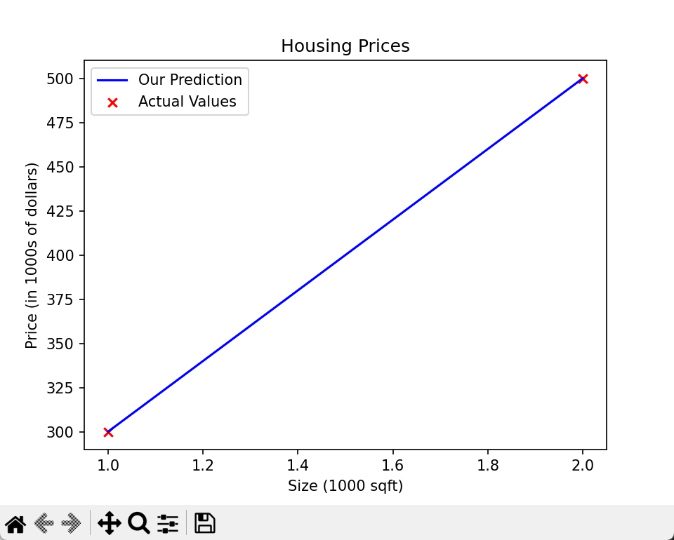
3.单变量线性回归案例(房屋面积预测价格)
import numpy as np
import matplotlib.pyplot as plt
from sklearn.linear_model import LinearRegression

# 1. 加载数据(面积:千平方英尺,价格:千美元)
X_train = np.array([1.0, 2.0])  # 特征
y_train = np.array([300, 500])  # 目标值

# 2. 创建并拟合模型
linear_model = LinearRegression()
# 注意:scikit-learn 的 fit 要求 X 是二维数组,所以用 reshape(-1,1) 转换
linear_model.fit(X_train.reshape(-1, 1), y_train)

# 3. 查看模型参数
b = linear_model.intercept_  # 截距项
w = linear_model.coef_      # 系数
print(f"w = {w}, b = {b:.2f}")
# 输出:w = [200.], b = 100.00

# 4. 手动验证预测
print(f"'manual' prediction: f_wb = wx+b : {1200*w + b}")
# 输出:'manual' prediction: f_wb = wx+b : [240100.]

# 5. 使用模型预测
# 训练集预测
y_pred = linear_model.predict(X_train.reshape(-1, 1))
print("Prediction on training set:", y_pred)
# 输出:Prediction on training set: [300. 500.]

# 新样本预测:1200平方英尺的房子
X_test = np.array([[1200]])
print(f"Prediction for 1200 sqft house: ${linear_model.predict(X_test)[0]:.2f}")
# 输出:Prediction for 1200 sqft house: $240100.00
结果解读
- 模型学习到的参数是 w=200,b=100,对应线性方程:价格(千美元)=200×面积(千平方英尺)+100
- 对 1200 平方英尺的房子(即 1.2 千平方英尺),预测价格为 200×1.2+100=340 千美元?这里注意:代码里的
1200*w + b是直接用 1200(平方英尺)计算,所以结果是 240100 美元,对应 240.1 千美元,本质是单位换算的小细节。
4.多变量线性回归案例(多特征房屋价格预测)
import numpy as np
from sklearn.linear_model import LinearRegression
from lab_utils_multi import load_house_data  # 题目提供的辅助函数

# 1. 加载数据集(多特征:面积、卧室数、楼层数、房龄)
X_train, y_train = load_house_data()
X_features = ['size(sqft)', 'bedrooms', 'floors', 'age']

# 2. 创建并拟合模型
linear_model = LinearRegression()
linear_model.fit(X_train, y_train)

# 3. 查看模型参数
b = linear_model.intercept_
w = linear_model.coef_
print(f"w = {w}, b = {b:.2f}")
# 输出:w = [  0.27 -32.62 -67.25  -1.47], b = 220.42

# 4. 验证预测结果
# 训练集预测(前4个样本)
print(f"Prediction on training set:\n {linear_model.predict(X_train)[:4]}")
print(f"prediction using w,b:\n {(X_train @ w + b)[:4]}")
print(f"Target values \n {y_train[:4]}")
# 输出:
# Prediction on training set: [295.18 485.98 389.52 492.15]
# prediction using w,b: [295.18 485.98 389.52 492.15]
# Target values [300.  509.8 394.  540. ]

# 5. 新样本预测:1200平方英尺、3卧室、1楼层、40年房龄的房子
x_house = np.array([1200, 3, 1, 40]).reshape(-1, 4)
x_house_predict = linear_model.predict(x_house)[0]
print(f"predicted price of a house with 1200 sqft, 3 bedrooms, 1 floor, 40 years old = ${x_house_predict*1000:.2f}")
# 输出:predicted price = $318709.09
关键细节
- 多变量模型的方程:价格(千美元)=0.27×面积−32.62×卧室数−67.25×楼层数−1.47×房龄+220.42
- 预测验证:
linear_model.predict(X_train)和手动计算X_train @ w + b结果完全一致,说明模型正确拟合了数据。 - 单位说明:预测结果乘以 1000 得到美元价格,例如 318.709 千美元对应 318709.09 美元。
4、两种方法对比:闭式解 vs 梯度下降
| 对比维度 | 闭式解(scikit-learn LinearRegression) | 梯度下降 |
|---|---|---|
| 实现方式 | 矩阵求逆,一步求解 | 迭代更新参数,逐步收敛 |
| 超参数 | 无(无需学习率、迭代次数) | 需设置学习率 α、迭代次数 |
| 特征处理 | 无需归一化 | 建议归一化特征,否则收敛慢 |
| 计算效率 | 小数据 / 少特征极快;大数据 / 多特征极慢 | 大数据 / 多特征更高效 |
| 适用场景 | 小数据集、特征数 n<104 | 大数据集、特征数多 |
5、常见问题与注意事项
-
X 必须是二维数组scikit-learn 的
fit方法要求输入特征X是二维矩阵(形状为(样本数, 特征数)),单变量数据需要用.reshape(-1, 1)转换,否则会报错。 -
多变量矩阵乘法多变量预测时,手动计算
X_train @ w + b用的是矩阵乘法,等价于对每个样本计算 ∑wixi+b,和predict方法的结果一致。 -
闭式解的局限性当特征数超过 10000 时,矩阵求逆的时间复杂度为 O(n3),计算成本会非常高,此时梯度下降是更优选择。

AtomGit 是由开放原子开源基金会联合 CSDN 等生态伙伴共同推出的新一代开源与人工智能协作平台。平台坚持“开放、中立、公益”的理念,把代码托管、模型共享、数据集托管、智能体开发体验和算力服务整合在一起,为开发者提供从开发、训练到部署的一站式体验。
更多推荐


 7
7 0
0- 0


 已为社区贡献3条内容

所有评论(0)