结构热应力仿真-主题096_量子计算在材料科学中的应用-主题096_量子计算在材料科学中的应用_完整教程
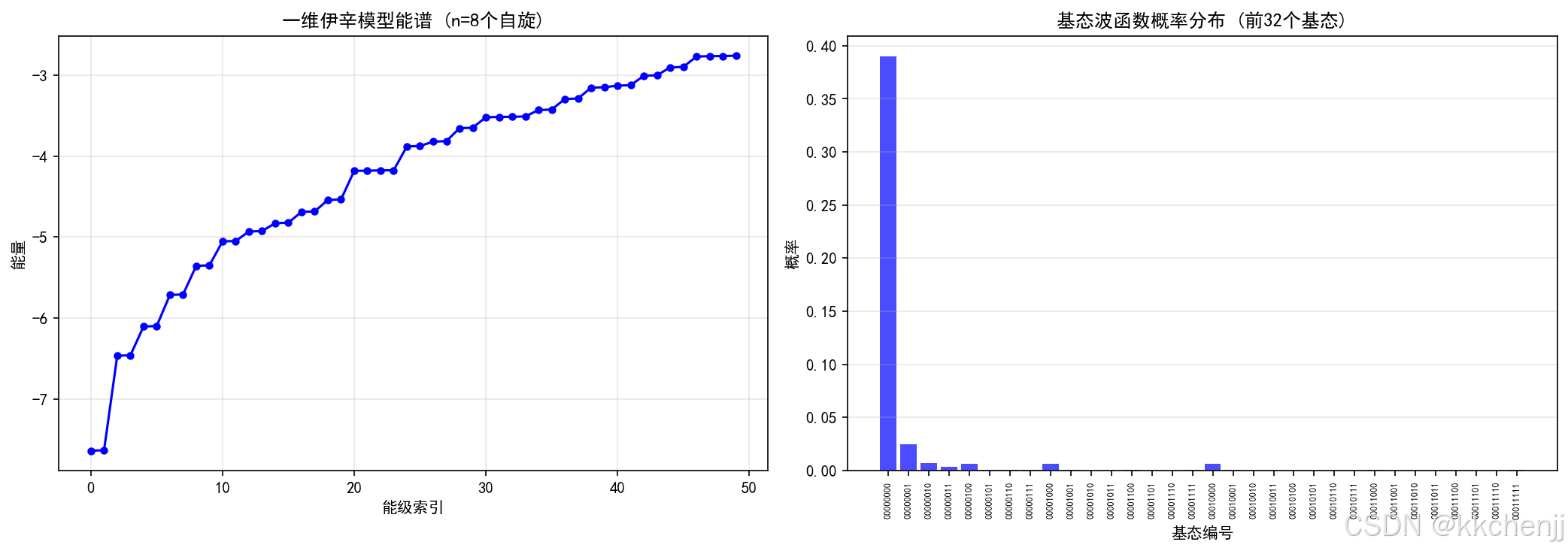

实例二:量子模拟在材料科学中的应用
6.1 实例概述
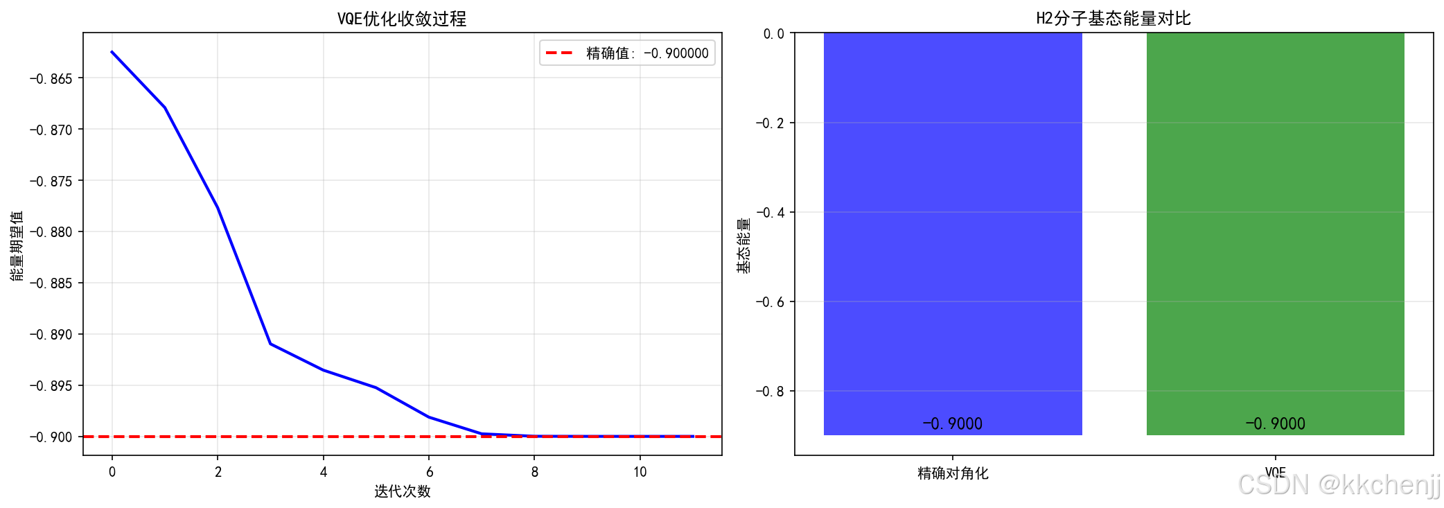
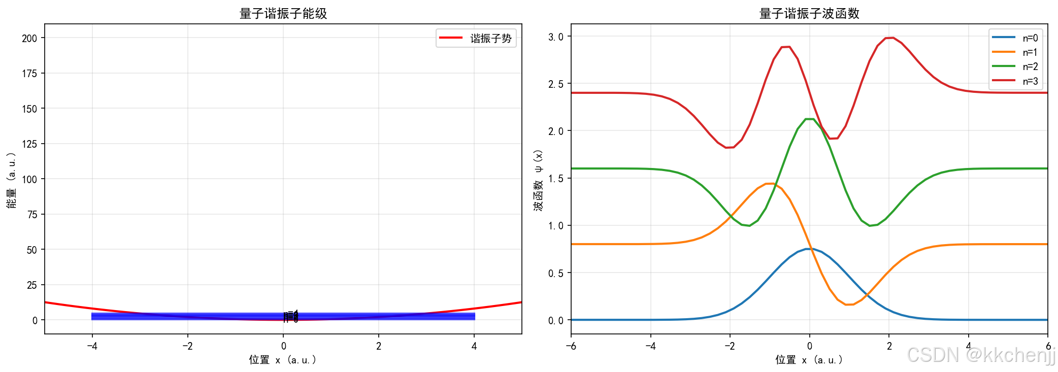
本实例演示如何使用经典计算机模拟量子系统,包括氢原子能级计算、量子谐振子、伊辛模型模拟以及变分量子本征求解器(VQE)的实现。
6.2 氢原子能级计算
氢原子是最简单的原子系统,其能级可以通过求解定态薛定谔方程得到:
H^ψ=Eψ\hat{H}\psi = E\psiH^ψ=Eψ
其中哈密顿量包含动能项和库仑势能项。通过有限差分法离散化后,可以构建哈密顿矩阵并求解本征值问题。
关键代码解析:
# 构建哈密顿矩阵
# 动能项(有限差分)
T = np.zeros((N, N))
for i in range(N):
    T[i, i] = 2.0
    if i > 0:
        T[i, i-1] = -1.0
    if i < N-1:
        T[i, i+1] = -1.0
T = T * (hbar**2 / (2 * m_e * dx**2))

# 势能项(库仑势)
V = np.zeros((N, N))
for i in range(N):
    if abs(x[i]) > 0.1:  # 避免奇点
        V[i, i] = -1.0 / abs(x[i])

# 求解本征值问题
eigenvalues, eigenvectors = eig(H)
6.3 变分量子本征求解器(VQE)
VQE是一种混合量子-经典算法,用于计算分子的基态能量。算法流程:
- 选择ansatz:参数化量子电路
- 制备试探态:∣ψ(θ)⟩|\psi(\theta)\rangle∣ψ(θ)⟩
- 测量期望值:E(θ)=⟨ψ(θ)∣H^∣ψ(θ)⟩E(\theta) = \langle\psi(\theta)|\hat{H}|\psi(\theta)\rangleE(θ)=⟨ψ(θ)∣H^∣ψ(θ)⟩
- 经典优化:更新参数θ\thetaθ
- 迭代直至收敛
VQE优势:
- 适合NISQ设备
- 电路深度较浅
- 对噪声有一定鲁棒性
实例三:量子优化算法实现
7.1 Grover搜索算法
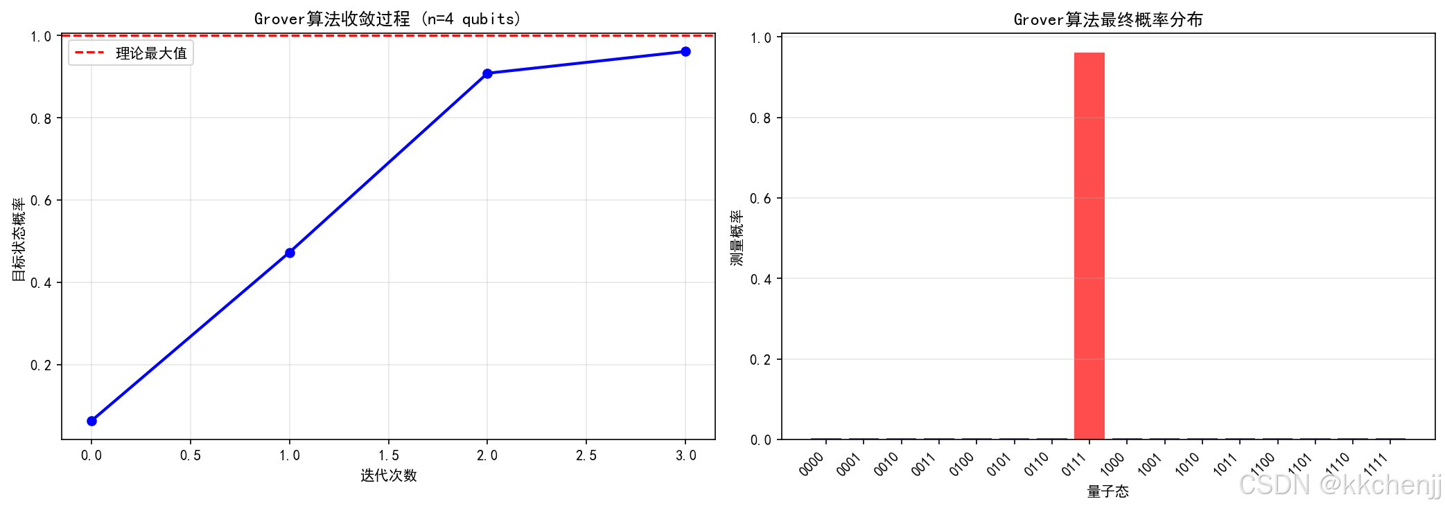
Grover算法在未排序数据库中搜索目标项,提供平方级加速:
- 经典复杂度:O(N)O(N)O(N)
- 量子复杂度:O(N)O(\sqrt{N})O(N)
算法步骤:
- 初始化均匀叠加态
- Oracle操作:标记目标状态
- 扩散操作:放大目标状态振幅
- 重复步骤2-3约π4N\frac{\pi}{4}\sqrt{N}4πN次
- 测量
7.2 量子近似优化算法(QAOA)
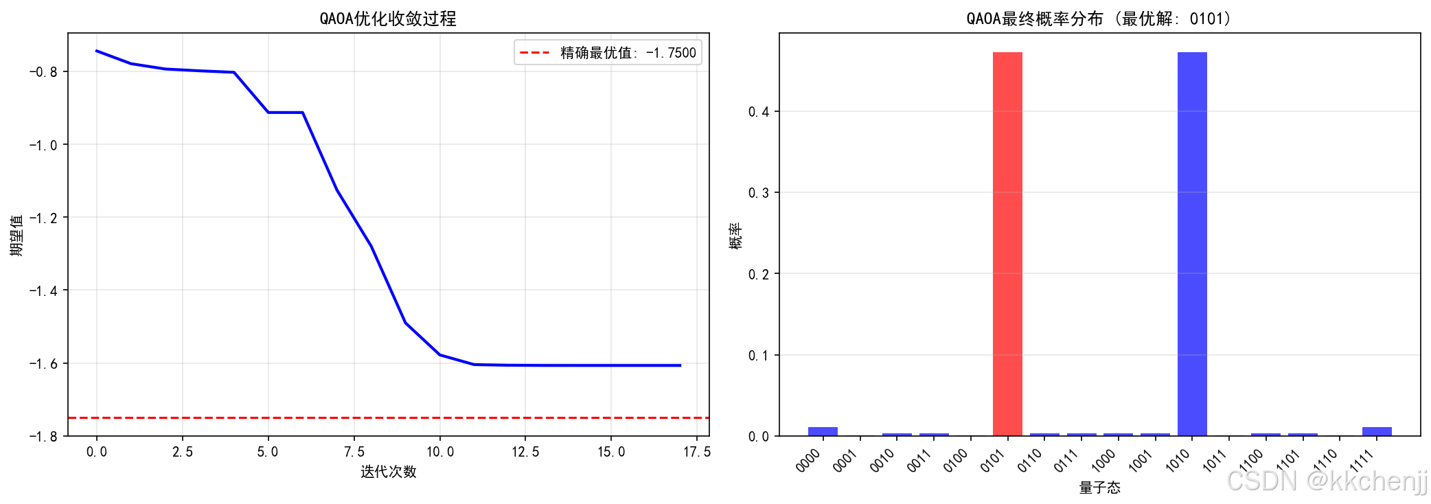
QAOA用于解决组合优化问题,如Max-Cut、TSP等。
核心思想:
将优化问题映射到伊辛模型哈密顿量:
HC=∑i,jJijZiZj+∑ihiZiH_C = \sum_{i,j} J_{ij} Z_i Z_j + \sum_i h_i Z_iHC=i,j∑JijZiZj+i∑hiZi
通过交替应用问题哈密顿量和混合哈密顿量的演化,逐步逼近最优解。
7.3 量子退火
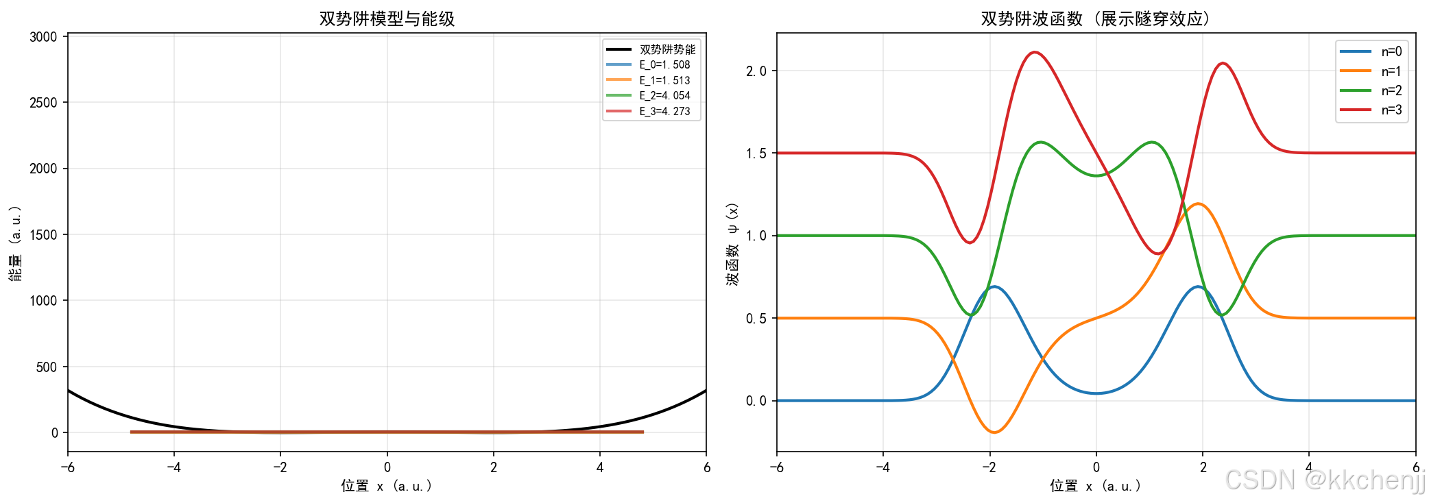
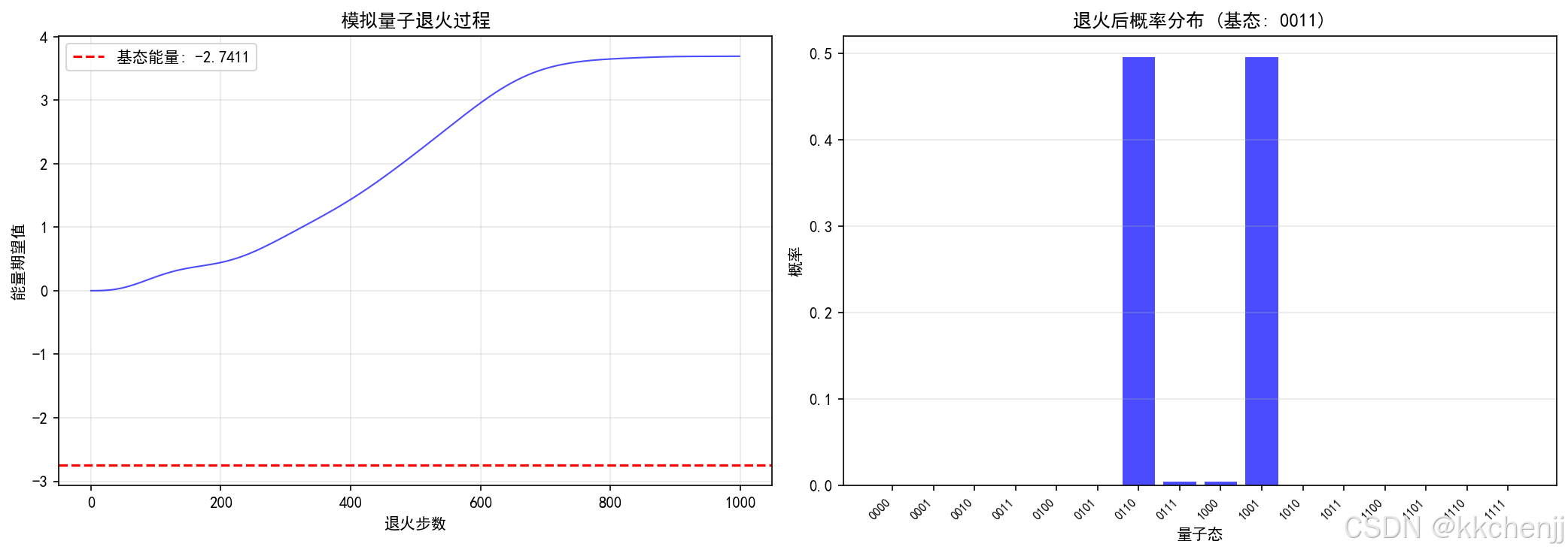
量子退火利用量子隧穿效应逃离局部最优解,在组合优化问题中表现出色。
退火过程:
H(t)=A(t)Hmixer+B(t)HproblemH(t) = A(t)H_{mixer} + B(t)H_{problem}H(t)=A(t)Hmixer+B(t)Hproblem
其中A(t)A(t)A(t)从大到小变化,B(t)B(t)B(t)从小到大变化。
实例四:量子机器学习在材料预测中的应用
8.1 量子特征映射
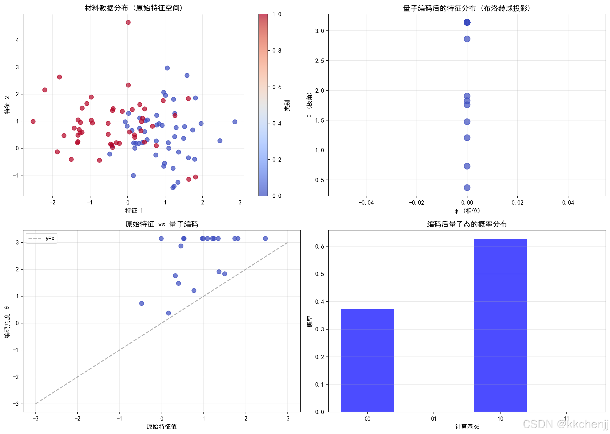
将经典数据编码到量子态是量子机器学习的第一步。常用方法:
角度编码:
∣ψ(x)⟩=⨂i=1nRY(xi)∣0⟩|\psi(x)\rangle = \bigotimes_{i=1}^n R_Y(x_i)|0\rangle∣ψ(x)⟩=i=1⨂nRY(xi)∣0⟩
幅度编码:
∣ψ(x)⟩=∑i=0N−1xi∣i⟩|\psi(x)\rangle = \sum_{i=0}^{N-1} x_i |i\rangle∣ψ(x)⟩=i=0∑N−1xi∣i⟩
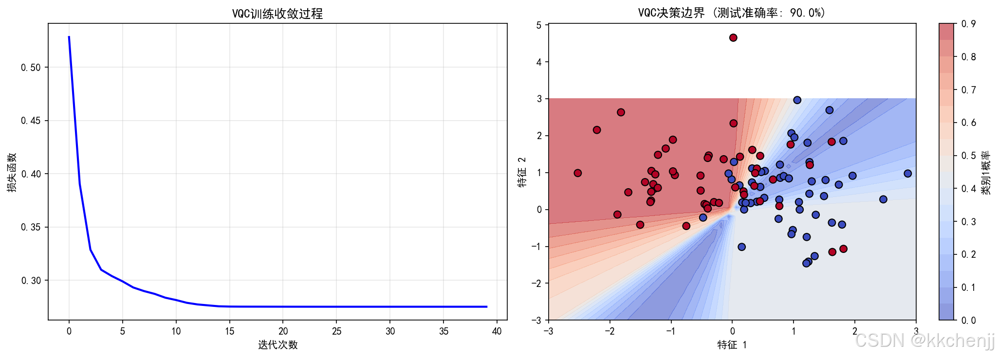
8.2 变分量子分类器(VQC)
VQC是一种参数化量子电路,可用于分类任务。
结构:
- 特征编码层
- 变分层(可训练参数)
- 测量层
训练:使用经典优化器最小化损失函数
8.3 量子核方法
量子核函数定义为两个量子态的重叠:
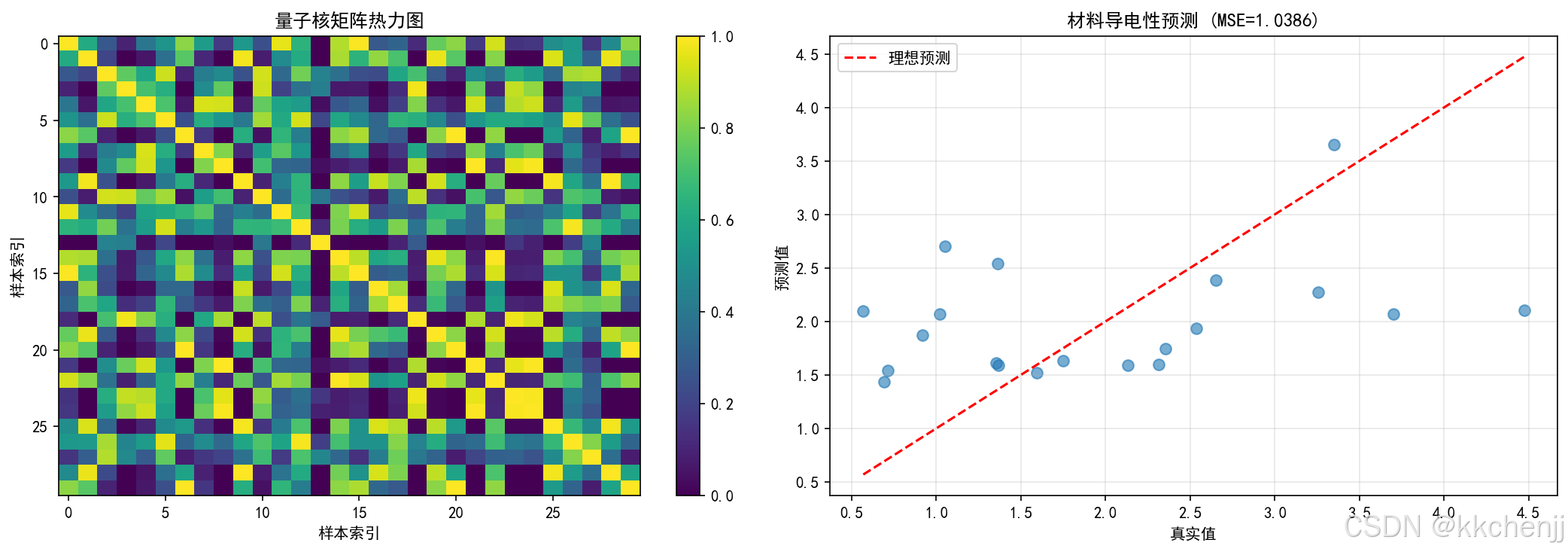
K(x1,x2)=∣⟨ϕ(x1)∣ϕ(x2)⟩∣2K(x_1, x_2) = |\langle\phi(x_1)|\phi(x_2)\rangle|^2K(x1,x2)=∣⟨ϕ(x1)∣ϕ(x2)⟩∣2
量子核可以捕捉经典方法难以表达的特征关系。
量子计算软件与平台
9.1 量子计算框架
| 框架 | 特点 | 适用场景 |
|---|---|---|
| Qiskit | IBM开发,功能全面 | 研究、教学、工业应用 |
| Cirq | Google开发,灵活 | 算法研究、NISQ实验 |
| PennyLane | 自动微分 | 量子机器学习 |
| ProjectQ | 开源、模块化 | 算法开发 |
| QuTiP | Python量子工具箱 | 量子动力学模拟 |
9.2 量子硬件平台
超导量子比特:
- IBM Quantum
- Google Sycamore
- Rigetti
离子阱:
- IonQ
- Honeywell
光量子:
- Xanadu
- PsiQuantum
中性原子:
- QuEra
- Pasqal
9.3 量子云服务
- IBM Quantum Experience:免费访问量子计算机
- Amazon Braket:统一量子计算平台
- Azure Quantum:微软量子云服务
- Google Quantum AI:量子算法研究
前沿研究与发展趋势
10.1 量子优势实现
2023-2024年的重要进展:
- 量子纠错:表面码、颜色码等纠错方案进展
- 逻辑量子比特:实现低错误率的逻辑量子比特
- 量子体积:量子计算机性能指标持续提升
10.2 材料科学应用前沿
当前研究热点:
- 高温超导:理解配对机制,预测新材料
- 催化剂设计:精确计算反应路径
- 电池材料:离子输运和电极反应模拟
- 光伏材料:光电转换效率预测
- 拓扑材料:拓扑不变量计算
10.3 量子-经典混合算法
NISQ时代的主流方法:
- VQE及其变种:UCCSD、ADAPT-VQE
- QAOA优化:参数优化、问题映射
- 量子机器学习:QSVM、QNN、量子核方法
10.4 未来展望
短期目标(2025-2030):
- 实现1000+物理量子比特
- 展示实际应用中的量子优势
- 开发更高效的量子算法
长期目标(2030+):
- 容错通用量子计算机
- 大规模材料模拟
- 新材料自主发现
总结与展望
11.1 核心知识点回顾
通过本教程的学习,我们掌握了:
- 量子计算基础:量子比特、量子门、量子电路
- 量子算法:Grover搜索、QAOA、VQE、量子模拟
- 材料科学应用:电子结构计算、材料优化、性质预测
- 量子机器学习:特征映射、变分分类器、量子核方法
11.2 量子计算在材料科学中的价值
理论优势:
- 指数级加速量子系统模拟
- 精确计算电子相关效应
- 处理强关联系统
实际应用:
- 加速新材料发现
- 优化材料性能
- 降低实验成本
11.3 学习建议
- 夯实基础:深入理解量子力学和线性代数
- 动手实践:使用Qiskit等框架实现算法
- 关注前沿:跟踪最新研究进展
- 跨学科学习:结合材料科学和量子计算
课后习题
基础题
-
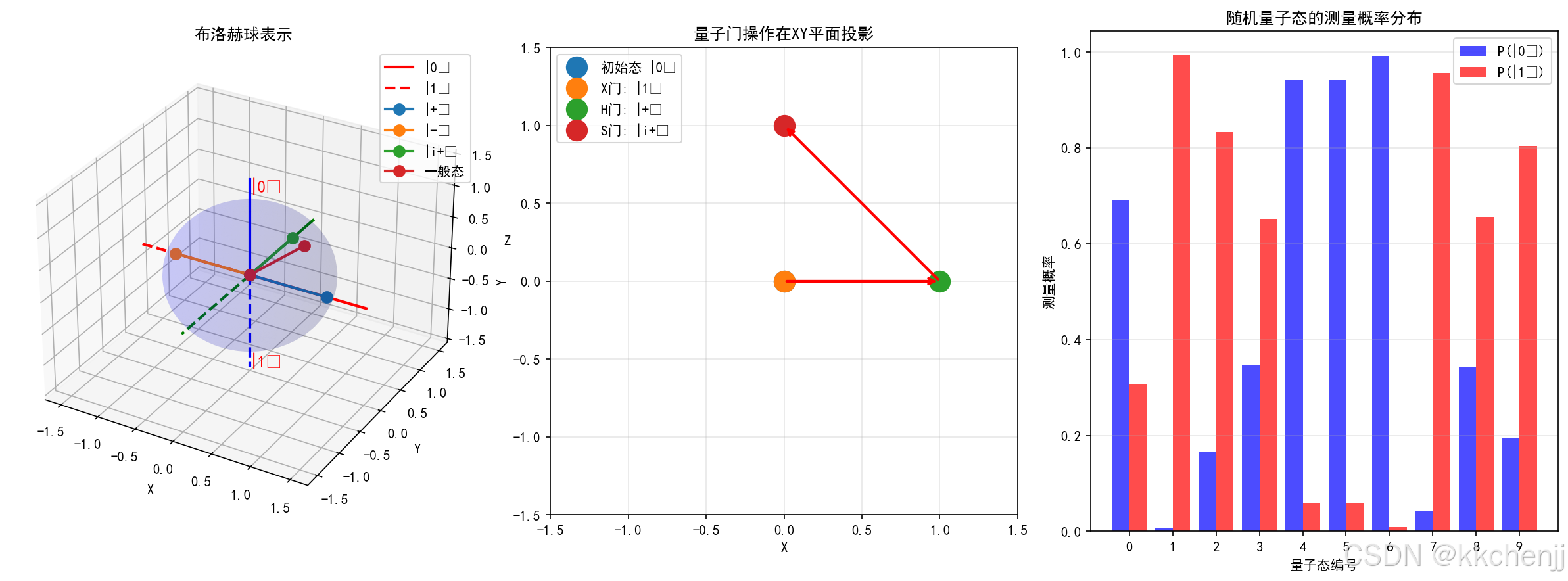
量子比特表示:证明任意单量子比特态可以表示为布洛赫球上的点。
-
量子门操作:验证Hadamard门是幺正的,并计算H∣0⟩H|0\rangleH∣0⟩和H∣1⟩H|1\rangleH∣1⟩。
-
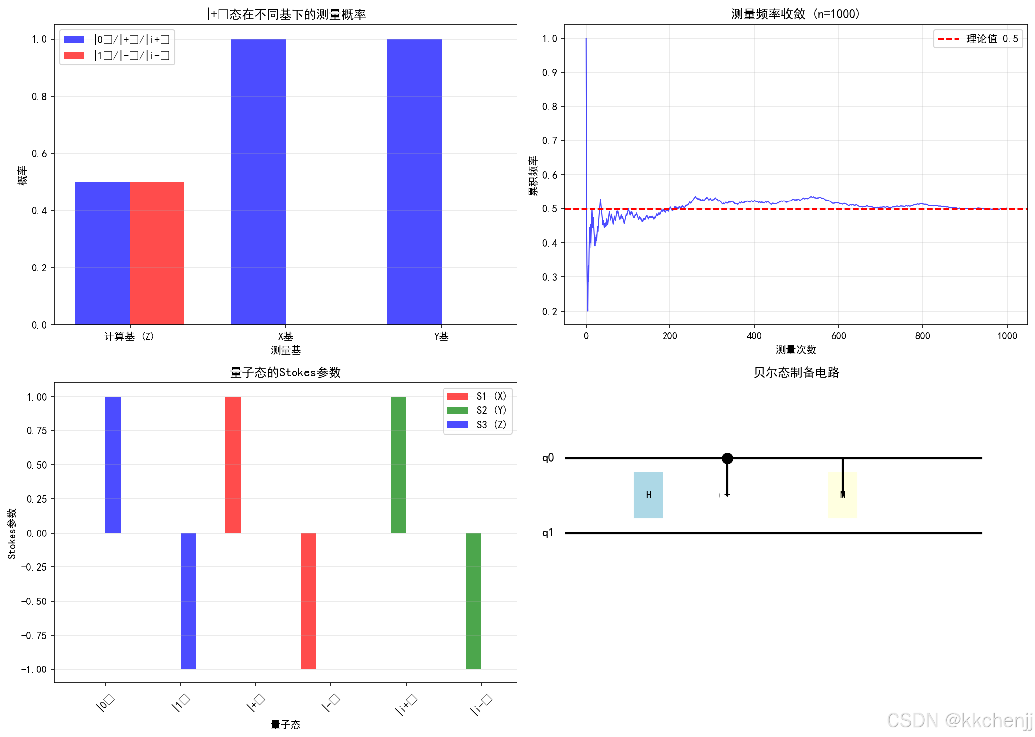
贝尔态制备:写出制备四个贝尔态的量子电路。
进阶题
-
Grover算法分析:推导Grover算法的最优迭代次数公式。
-
VQE实现:使用Python实现一个简单的VQE算法,求解氢分子基态能量。
-
QAOA应用:将Max-Cut问题映射到伊辛模型,并实现QAOA求解。
挑战题
-
量子模拟:使用Trotter分解模拟氢原子的时间演化。
-
量子机器学习:实现一个量子核支持向量机,并与经典方法对比。
-
材料应用:选择一个实际材料问题,设计量子算法解决方案。
参考文献
量子计算基础
-
Nielsen, M. A., & Chuang, I. L. (2010). Quantum Computation and Quantum Information. Cambridge University Press.
-
Preskill, J. (2018). Quantum Computing in the NISQ era and beyond. Quantum, 2, 79.
量子算法
-
Shor, P. W. (1994). Algorithms for quantum computation. Proceedings 35th Annual Symposium on Foundations of Computer Science.
-
Grover, L. K. (1996). A fast quantum mechanical algorithm for database search. Proceedings 28th Annual ACM Symposium on Theory of Computing.
-
Peruzzo, A., et al. (2014). A variational eigenvalue solver on a photonic quantum processor. Nature Communications, 5, 4213.
量子计算与材料科学
-
Cao, Y., et al. (2019). Quantum chemistry in the age of quantum computing. Chemical Reviews, 119(19), 10856-10915.
-
McArdle, S., et al. (2020). Quantum computational chemistry. Reviews of Modern Physics, 92(1), 015003.
-
Bauer, B., et al. (2020). Quantum algorithms for quantum chemistry and quantum materials science. Chemical Reviews, 120(22), 12685-12717.
量子机器学习
-
Biamonte, J., et al. (2017). Quantum machine learning. Nature, 549(7671), 195-202.
-
Schuld, M., & Petruccione, F. (2021). Machine Learning with Quantum Computers. Springer.
附录
附录A:常用量子门矩阵
单量子比特门:
X=(0110),Y=(0−ii0),Z=(100−1)X = \begin{pmatrix} 0 & 1 \\ 1 & 0 \end{pmatrix}, \quad Y = \begin{pmatrix} 0 & -i \\ i & 0 \end{pmatrix}, \quad Z = \begin{pmatrix} 1 & 0 \\ 0 & -1 \end{pmatrix}X=(0110),Y=(0i−i0),Z=(100−1)
H=12(111−1),S=(100i),T=(100eiπ/4)H = \frac{1}{\sqrt{2}}\begin{pmatrix} 1 & 1 \\ 1 & -1 \end{pmatrix}, \quad S = \begin{pmatrix} 1 & 0 \\ 0 & i \end{pmatrix}, \quad T = \begin{pmatrix} 1 & 0 \\ 0 & e^{i\pi/4} \end{pmatrix}H=21(111−1),S=(100i),T=(100eiπ/4)
旋转门:
Rx(θ)=(cosθ2−isinθ2−isinθ2cosθ2)R_x(\theta) = \begin{pmatrix} \cos\frac{\theta}{2} & -i\sin\frac{\theta}{2} \\ -i\sin\frac{\theta}{2} & \cos\frac{\theta}{2} \end{pmatrix}Rx(θ)=(cos2θ−isin2θ−isin2θcos2θ)
Ry(θ)=(cosθ2−sinθ2sinθ2cosθ2)R_y(\theta) = \begin{pmatrix} \cos\frac{\theta}{2} & -\sin\frac{\theta}{2} \\ \sin\frac{\theta}{2} & \cos\frac{\theta}{2} \end{pmatrix}Ry(θ)=(cos2θsin2θ−sin2θcos2θ)
Rz(θ)=(e−iθ/200eiθ/2)R_z(\theta) = \begin{pmatrix} e^{-i\theta/2} & 0 \\ 0 & e^{i\theta/2} \end{pmatrix}Rz(θ)=(e−iθ/200eiθ/2)
多量子比特门:
CNOT=(1000010000010010)CNOT = \begin{pmatrix} 1 & 0 & 0 & 0 \\ 0 & 1 & 0 & 0 \\ 0 & 0 & 0 & 1 \\ 0 & 0 & 1 & 0 \end{pmatrix}CNOT= 1000010000010010
SWAP=(1000001001000001)SWAP = \begin{pmatrix} 1 & 0 & 0 & 0 \\ 0 & 0 & 1 & 0 \\ 0 & 1 & 0 & 0 \\ 0 & 0 & 0 & 1 \end{pmatrix}SWAP= 1000001001000001
附录B:Python代码模板
量子态制备:
import numpy as np

# 创建量子态
def create_quantum_state(amplitudes):
    """创建归一化的量子态"""
    state = np.array(amplitudes, dtype=complex)
    return state / np.linalg.norm(state)

# 应用量子门
def apply_gate(state, gate):
    """应用量子门到量子态"""
    return gate @ state
量子测量:
def measure_state(state, n_shots=1000):
    """模拟量子测量"""
    probabilities = np.abs(state)**2
    n_qubits = int(np.log2(len(state)))

    outcomes = np.random.choice(
        range(2**n_qubits),
        size=n_shots,
        p=probabilities
    )
    return outcomes
"""
实例一:量子计算基础与量子门操作
"""
import numpy as np
import matplotlib
matplotlib.use('Agg')  # 使用非交互式后端
import matplotlib.pyplot as plt
from mpl_toolkits.mplot3d import Axes3D

# 设置中文字体
plt.rcParams['font.sans-serif'] = ['SimHei', 'DejaVu Sans']
plt.rcParams['axes.unicode_minus'] = False

print("=" * 60)
print("量子计算基础与量子门操作")
print("=" * 60)

# ============================================================
# 1. 量子态表示与布洛赫球可视化
# ============================================================
print("\n【1】量子态表示与布洛赫球可视化...")

# 定义量子态
def bloch_coordinates(state):
    """从量子态计算布洛赫球坐标"""
    alpha, beta = state
    # 计算布洛赫球坐标
    theta = 2 * np.arccos(np.abs(alpha))
    phi = np.angle(beta) - np.angle(alpha)
    return theta, phi

def state_vector(theta, phi):
    """从布洛赫球坐标生成量子态"""
    alpha = np.cos(theta / 2)
    beta = np.exp(1j * phi) * np.sin(theta / 2)
    return np.array([alpha, beta])

# 创建布洛赫球可视化
fig = plt.figure(figsize=(16, 6))

# 布洛赫球
ax1 = fig.add_subplot(131, projection='3d')

# 绘制球面
u = np.linspace(0, 2 * np.pi, 50)
v = np.linspace(0, np.pi, 50)
x_sphere = np.outer(np.cos(u), np.sin(v))
y_sphere = np.outer(np.sin(u), np.sin(v))
z_sphere = np.outer(np.ones(np.size(u)), np.cos(v))
ax1.plot_surface(x_sphere, y_sphere, z_sphere, alpha=0.1, color='blue')

# 绘制坐标轴
ax1.plot([0, 1.5], [0, 0], [0, 0], 'r-', linewidth=2, label='|0⟩')
ax1.plot([0, -1.5], [0, 0], [0, 0], 'r--', linewidth=2, label='|1⟩')
ax1.plot([0, 0], [0, 1.5], [0, 0], 'g-', linewidth=2)
ax1.plot([0, 0], [0, -1.5], [0, 0], 'g--', linewidth=2)
ax1.plot([0, 0], [0, 0], [0, 1.5], 'b-', linewidth=2)
ax1.plot([0, 0], [0, 0], [0, -1.5], 'b--', linewidth=2)

# 标记基态
ax1.text(0, 0, 1.3, '|0⟩', fontsize=12, color='red')
ax1.text(0, 0, -1.5, '|1⟩', fontsize=12, color='red')

# 绘制几个量子态
states_to_plot = [
    (np.pi/2, 0, '|+⟩'),
    (np.pi/2, np.pi, '|-⟩'),
    (np.pi/2, np.pi/2, '|i+⟩'),
    (np.pi/4, 0, '一般态'),
]

for theta, phi, label in states_to_plot:
    x = np.sin(theta) * np.cos(phi)
    y = np.sin(theta) * np.sin(phi)
    z = np.cos(theta)
    ax1.plot([0, x], [0, y], [0, z], 'o-', markersize=8, linewidth=2, label=label)

ax1.set_xlabel('X')
ax1.set_ylabel('Y')
ax1.set_zlabel('Z')
ax1.set_title('布洛赫球表示')
ax1.legend()

# 量子门操作可视化
ax2 = fig.add_subplot(132)

# 初始态 |0>
theta_0, phi_0 = 0, 0
states = [(theta_0, phi_0, '初始态 |0⟩')]

# X门操作 (|0> -> |1>)
theta_x, phi_x = np.pi, 0
states.append((theta_x, phi_x, 'X门: |1⟩'))

# H门操作 (|0> -> |+>)
theta_h, phi_h = np.pi/2, 0
states.append((theta_h, phi_h, 'H门: |+⟩'))

# S门操作 (|+> -> |i+>)
theta_s, phi_s = np.pi/2, np.pi/2
states.append((theta_s, phi_s, 'S门: |i+⟩'))

# 绘制状态演化
for i, (theta, phi, label) in enumerate(states):
    x = np.sin(theta) * np.cos(phi)
    y = np.sin(theta) * np.sin(phi)
    ax2.plot(x, y, 'o', markersize=15, label=label)
    if i > 0:
        prev_x = np.sin(states[i-1][0]) * np.cos(states[i-1][1])
        prev_y = np.sin(states[i-1][0]) * np.sin(states[i-1][1])
        ax2.annotate('', xy=(x, y), xytext=(prev_x, prev_y),
                    arrowprops=dict(arrowstyle='->', lw=2, color='red'))

ax2.set_xlim(-1.5, 1.5)
ax2.set_ylim(-1.5, 1.5)
ax2.set_xlabel('X')
ax2.set_ylabel('Y')
ax2.set_title('量子门操作在XY平面投影')
ax2.legend()
ax2.grid(True, alpha=0.3)
ax2.set_aspect('equal')

# 概率幅可视化
ax3 = fig.add_subplot(133)

# 生成随机量子态
np.random.seed(42)
n_states = 10
theta_vals = np.random.uniform(0, np.pi, n_states)
phi_vals = np.random.uniform(0, 2*np.pi, n_states)

x_pos = np.arange(n_states)
prob_0 = np.cos(theta_vals/2)**2
prob_1 = np.sin(theta_vals/2)**2

ax3.bar(x_pos - 0.2, prob_0, 0.4, label='P(|0⟩)', color='blue', alpha=0.7)
ax3.bar(x_pos + 0.2, prob_1, 0.4, label='P(|1⟩)', color='red', alpha=0.7)

ax3.set_xlabel('量子态编号')
ax3.set_ylabel('测量概率')
ax3.set_title('随机量子态的测量概率分布')
ax3.set_xticks(x_pos)
ax3.legend()
ax3.grid(True, alpha=0.3, axis='y')

plt.tight_layout()
plt.savefig('量子计算基础_布洛赫球与量子门.png', dpi=150, bbox_inches='tight')
plt.close()

print("  已保存: 量子计算基础_布洛赫球与量子门.png")

# ============================================================
# 2. 量子门矩阵表示
# ============================================================
print("\n【2】量子门矩阵表示...")

# 定义量子门
I = np.array([[1, 0], [0, 1]])
X = np.array([[0, 1], [1, 0]])
Y = np.array([[0, -1j], [1j, 0]])
Z = np.array([[1, 0], [0, -1]])
H = np.array([[1, 1], [1, -1]]) / np.sqrt(2)
S = np.array([[1, 0], [0, 1j]])
T = np.array([[1, 0], [0, np.exp(1j*np.pi/4)]])

print("  常用量子门矩阵:")
print(f"  X门 (NOT):\n{X}")
print(f"  Z门:\n{Z}")
print(f"  H门 (Hadamard):\n{H.round(4)}")

# 验证门的性质
print("\n  验证幺正性 (U†U = I):")
print(f"  X†X = {np.allclose(X.conj().T @ X, I)}")
print(f"  H†H = {np.allclose(H.conj().T @ H, I)}")

# 门操作效果
print("\n  门操作效果:")
state_0 = np.array([1, 0])
state_1 = np.array([0, 1])

print(f"  X|0⟩ = {X @ state_0}")
print(f"  X|1⟩ = {X @ state_1}")
print(f"  H|0⟩ = {H @ state_0}")
print(f"  H|1⟩ = {H @ state_1}")

# ============================================================
# 3. 多量子比特系统
# ============================================================
print("\n【3】多量子比特系统...")

# CNOT门
CNOT = np.array([[1, 0, 0, 0],
                 [0, 1, 0, 0],
                 [0, 0, 0, 1],
                 [0, 0, 1, 0]])

print("  CNOT门矩阵:")
print(CNOT)

# 贝尔态制备
# |Φ+⟩ = (|00⟩ + |11⟩)/√2
state_00 = np.array([1, 0, 0, 0])
bell_state = CNOT @ np.kron(H, I) @ state_00

print(f"\n  贝尔态 |Φ+⟩ = (|00⟩ + |11⟩)/√2:")
print(f"  态矢量: {bell_state}")
print(f"  验证归一化: {np.sum(np.abs(bell_state)**2)}")

# 验证纠缠
# 贝尔态不能写成单量子比特态的直积
print(f"\n  贝尔态是纠缠态 (无法分解)")

# ============================================================
# 4. 量子测量统计
# ============================================================
print("\n【4】量子测量统计模拟...")

# 创建可视化
fig, axes = plt.subplots(2, 2, figsize=(14, 10))

# 测量不同基态
bases = ['计算基 (Z)', 'X基', 'Y基']
measurements = []

# |+⟩态在不同基下的测量
state_plus = np.array([1, 1]) / np.sqrt(2)

# Z基测量
prob_z = np.abs(state_plus)**2
measurements.append(prob_z)

# X基测量 (转换到X基)
H_dagger = H.conj().T
state_plus_x = H_dagger @ state_plus
prob_x = np.abs(state_plus_x)**2
measurements.append(prob_x)

# Y基测量
S_dagger = S.conj().T
state_plus_y = S_dagger @ H_dagger @ state_plus
prob_y = np.abs(state_plus_y)**2
measurements.append(prob_y)

# 绘制测量概率
ax1 = axes[0, 0]
x = np.arange(len(bases))
width = 0.35
ax1.bar(x - width/2, [m[0] for m in measurements], width, label='|0⟩/|+⟩/|i+⟩', color='blue', alpha=0.7)
ax1.bar(x + width/2, [m[1] for m in measurements], width, label='|1⟩/|-⟩/|i-⟩', color='red', alpha=0.7)
ax1.set_xlabel('测量基')
ax1.set_ylabel('概率')
ax1.set_title('|+⟩态在不同基下的测量概率')
ax1.set_xticks(x)
ax1.set_xticklabels(bases)
ax1.legend()
ax1.grid(True, alpha=0.3, axis='y')

# 多次测量统计
ax2 = axes[0, 1]
n_shots = 1000
outcomes = np.random.choice([0, 1], size=n_shots, p=[0.5, 0.5])
cumulative = np.cumsum(outcomes) / np.arange(1, n_shots + 1)

ax2.plot(cumulative, 'b-', linewidth=1, alpha=0.7)
ax2.axhline(y=0.5, color='r', linestyle='--', label='理论值 0.5')
ax2.set_xlabel('测量次数')
ax2.set_ylabel('累积频率')
ax2.set_title(f'测量频率收敛 (n={n_shots})')
ax2.legend()
ax2.grid(True, alpha=0.3)

# 量子态层析
ax3 = axes[1, 0]

# 模拟不同量子态的测量
states_labels = ['|0⟩', '|1⟩', '|+⟩', '|-⟩', '|i+⟩', '|i-⟩']
states_list = [
    np.array([1, 0]),
    np.array([0, 1]),
    np.array([1, 1])/np.sqrt(2),
    np.array([1, -1])/np.sqrt(2),
    np.array([1, 1j])/np.sqrt(2),
    np.array([1, -1j])/np.sqrt(2),
]

# 计算Stokes参数
S0, S1, S2, S3 = [], [], [], []
for state in states_list:
    rho = np.outer(state, state.conj())
    S0.append(np.trace(rho).real)
    S1.append(np.trace(rho @ X).real)
    S2.append(np.trace(rho @ Y).real)
    S3.append(np.trace(rho @ Z).real)

x = np.arange(len(states_labels))
ax3.bar(x - 0.3, S1, 0.2, label='S1 (X)', color='red', alpha=0.7)
ax3.bar(x - 0.1, S2, 0.2, label='S2 (Y)', color='green', alpha=0.7)
ax3.bar(x + 0.1, S3, 0.2, label='S3 (Z)', color='blue', alpha=0.7)
ax3.set_xlabel('量子态')
ax3.set_ylabel('Stokes参数')
ax3.set_title('量子态的Stokes参数')
ax3.set_xticks(x)
ax3.set_xticklabels(states_labels, rotation=45)
ax3.legend()
ax3.grid(True, alpha=0.3, axis='y')

# 量子电路示意
ax4 = axes[1, 1]
ax4.set_xlim(0, 10)
ax4.set_ylim(0, 4)

# 绘制量子线
for i in range(2):
    ax4.plot([0, 9], [3-i, 3-i], 'k-', linewidth=2)
    ax4.text(-0.5, 3-i, f'q{i}', fontsize=12, va='center')

# H门
ax4.add_patch(plt.Rectangle((1.5, 2.2), 0.6, 0.6, fill=True, color='lightblue', edgecolor='black'))
ax4.text(1.8, 2.5, 'H', fontsize=10, ha='center', va='center')

# CNOT门
ax4.plot([3.5, 3.5], [2.5, 3], 'k-', linewidth=2)
ax4.plot(3.5, 3, 'ko', markersize=10)
ax4.add_patch(plt.Circle((3.5, 2.5), 0.15, fill=True, color='black'))
ax4.add_patch(plt.Rectangle((3.35, 2.35), 0.3, 0.3, fill=True, color='white', edgecolor='black'))
ax4.text(3.5, 2.5, '+', fontsize=12, ha='center', va='center')

# 测量
ax4.plot([6, 6], [2.5, 3], 'k-', linewidth=2)
ax4.add_patch(plt.Rectangle((5.7, 2.2), 0.6, 0.6, fill=True, color='lightyellow', edgecolor='black'))
ax4.text(6, 2.5, 'M', fontsize=10, ha='center', va='center')

ax4.set_title('贝尔态制备电路')
ax4.axis('off')

plt.tight_layout()
plt.savefig('量子计算基础_测量与层析.png', dpi=150, bbox_inches='tight')
plt.close()

print("  已保存: 量子计算基础_测量与层析.png")

print("\n" + "=" * 60)
print("量子计算基础演示完成!")
print("=" * 60)
"""
实例二:量子模拟在材料科学中的应用
本实例演示如何使用经典计算机模拟量子系统,包括:
- 氢原子能级计算
- 谐振子问题
- 伊辛模型模拟
- VQE算法演示
"""
import numpy as np
import matplotlib
matplotlib.use('Agg')  # 使用非交互式后端
import matplotlib.pyplot as plt
from scipy.linalg import expm, eig
from scipy.optimize import minimize
from scipy.integrate import trapezoid

# 设置中文字体
plt.rcParams['font.sans-serif'] = ['SimHei', 'DejaVu Sans']
plt.rcParams['axes.unicode_minus'] = False

print("=" * 70)
print("量子模拟在材料科学中的应用")
print("=" * 70)

# ============================================================
# 1. 氢原子能级计算(一维简化模型)
# ============================================================
print("\n【1】氢原子能级计算(一维简化模型)...")

# 参数设置
hbar = 1.0  # 约化普朗克常数
m_e = 1.0   # 电子质量
a0 = 1.0    # 玻尔半径
N = 200     # 网格点数
x_max = 20  # 计算域范围

# 空间离散化
x = np.linspace(-x_max, x_max, N)
dx = x[1] - x[0]

# 构建哈密顿矩阵
# 动能项(有限差分)
T = np.zeros((N, N))
for i in range(N):
    T[i, i] = 2.0
    if i > 0:
        T[i, i-1] = -1.0
    if i < N-1:
        T[i, i+1] = -1.0
T = T * (hbar**2 / (2 * m_e * dx**2))

# 势能项(库仑势)
V = np.zeros((N, N))
for i in range(N):
    if abs(x[i]) > 0.1:  # 避免奇点
        V[i, i] = -1.0 / abs(x[i])
    else:
        V[i, i] = -10.0  # 截断处理

# 总哈密顿量
H = T + V

# 求解本征值问题
eigenvalues, eigenvectors = eig(H)
idx = eigenvalues.argsort()
eigenvalues = eigenvalues[idx].real
eigenvectors = eigenvectors[:, idx]

# 提取前几个能级
n_levels = 5
energy_levels = eigenvalues[:n_levels]
print(f"\n  前{n_levels}个能级 (原子单位):")
for i, E in enumerate(energy_levels):
    print(f"    n={i+1}: E = {E:.4f} (理论值: {-0.5/(i+1)**2:.4f})")

# 可视化
fig, axes = plt.subplots(1, 2, figsize=(14, 5))

# 能级图
ax1 = axes[0]
for i, E in enumerate(energy_levels):
    ax1.axhline(y=E, color='blue', linewidth=2, alpha=0.7)
    ax1.text(x_max*0.7, E, f'n={i+1}, E={E:.3f}', va='center', fontsize=10)

ax1.plot(x, np.diag(V), 'r--', linewidth=2, label='库仑势')
ax1.set_xlabel('位置 x (a.u.)')
ax1.set_ylabel('能量 (a.u.)')
ax1.set_title('氢原子能级(一维简化模型)')
ax1.set_xlim(-x_max, x_max)
ax1.set_ylim(-2, 1)
ax1.legend()
ax1.grid(True, alpha=0.3)

# 波函数
ax2 = axes[1]
for i in range(min(3, n_levels)):
    psi = eigenvectors[:, i].real
    # 归一化
    psi = psi / np.sqrt(trapezoid(psi**2, x))
    ax2.plot(x, psi + i*0.5, linewidth=2, label=f'n={i+1}')
    ax2.axhline(y=i*0.5, color='gray', linestyle='--', alpha=0.3)

ax2.set_xlabel('位置 x (a.u.)')
ax2.set_ylabel('波函数 ψ(x)')
ax2.set_title('氢原子波函数')
ax2.set_xlim(-x_max, x_max)
ax2.legend()
ax2.grid(True, alpha=0.3)

plt.tight_layout()
plt.savefig('量子模拟_氢原子能级.png', dpi=150, bbox_inches='tight')
plt.close()

print("  已保存: 量子模拟_氢原子能级.png")

# ============================================================
# 2. 量子谐振子
# ============================================================
print("\n【2】量子谐振子...")

# 谐振子参数
omega = 1.0  # 角频率

# 构建哈密顿矩阵
V_ho = np.zeros((N, N))
for i in range(N):
    V_ho[i, i] = 0.5 * m_e * omega**2 * x[i]**2

H_ho = T + V_ho

# 求解本征值
eigenvalues_ho, eigenvectors_ho = eig(H_ho)
idx_ho = eigenvalues_ho.argsort()
eigenvalues_ho = eigenvalues_ho[idx_ho].real
eigenvectors_ho = eigenvectors_ho[:, idx_ho]

print(f"\n  前5个能级 (理论值: E_n = (n+1/2)ℏω):")
for i in range(5):
    E_theory = (i + 0.5) * hbar * omega
    E_numerical = eigenvalues_ho[i]
    print(f"    n={i}: 数值 = {E_numerical:.4f}, 理论 = {E_theory:.4f}")

# 可视化
fig, axes = plt.subplots(1, 2, figsize=(14, 5))

# 能级与势能
ax1 = axes[0]
ax1.plot(x, np.diag(V_ho), 'r-', linewidth=2, label='谐振子势')
for i in range(5):
    E = eigenvalues_ho[i]
    ax1.axhline(y=E, xmin=0.1, xmax=0.9, color='blue', linewidth=2, alpha=0.7)
    ax1.text(0, E, f'n={i}', va='center', fontsize=10)

ax1.set_xlabel('位置 x (a.u.)')
ax1.set_ylabel('能量 (a.u.)')
ax1.set_title('量子谐振子能级')
ax1.set_xlim(-5, 5)
ax1.legend()
ax1.grid(True, alpha=0.3)

# 波函数
ax2 = axes[1]
for i in range(4):
    psi = eigenvectors_ho[:, i].real
    psi = psi / np.sqrt(trapezoid(psi**2, x))
    ax2.plot(x, psi + i*0.8, linewidth=2, label=f'n={i}')

ax2.set_xlabel('位置 x (a.u.)')
ax2.set_ylabel('波函数 ψ(x)')
ax2.set_title('量子谐振子波函数')
ax2.set_xlim(-6, 6)
ax2.legend()
ax2.grid(True, alpha=0.3)

plt.tight_layout()
plt.savefig('量子模拟_谐振子.png', dpi=150, bbox_inches='tight')
plt.close()

print("  已保存: 量子模拟_谐振子.png")

# ============================================================
# 3. 一维伊辛模型
# ============================================================
print("\n【3】一维伊辛模型模拟...")

# 伊辛模型参数
n_spins = 8  # 自旋数
J = 1.0      # 耦合常数
h = 0.5      # 外磁场

# 构建泡利矩阵
sigma_x = np.array([[0, 1], [1, 0]])
sigma_z = np.array([[1, 0], [0, -1]])
sigma_i = np.eye(2)

def tensor_product(matrices):
    """计算多个矩阵的张量积"""
    result = matrices[0]
    for mat in matrices[1:]:
        result = np.kron(result, mat)
    return result

# 构建哈密顿量
H_ising = np.zeros((2**n_spins, 2**n_spins))

# 自旋-自旋相互作用项
for i in range(n_spins - 1):
    matrices = [sigma_i] * n_spins
    matrices[i] = sigma_z
    matrices[i+1] = sigma_z
    H_ising += -J * tensor_product(matrices)

# 外磁场项
for i in range(n_spins):
    matrices = [sigma_i] * n_spins
    matrices[i] = sigma_x
    H_ising += -h * tensor_product(matrices)

# 求解基态
E_ising, psi_ising = eig(H_ising)
idx_ising = E_ising.argsort()
E_ising = E_ising[idx_ising].real
psi_ising = psi_ising[:, idx_ising]

print(f"\n  基态能量: {E_ising[0]:.4f}")
print(f"  第一激发态能量: {E_ising[1]:.4f}")
print(f"  能隙: {E_ising[1] - E_ising[0]:.4f}")

# 计算基态的磁化强度
magnetization = 0
for i in range(n_spins):
    matrices = [sigma_i] * n_spins
    matrices[i] = sigma_z
    sigma_z_i = tensor_product(matrices)
    magnetization += np.abs(psi_ising[:, 0].conj() @ sigma_z_i @ psi_ising[:, 0])

print(f"  基态磁化强度: {magnetization/n_spins:.4f}")

# 可视化
fig, axes = plt.subplots(1, 2, figsize=(14, 5))

# 能谱
ax1 = axes[0]
ax1.plot(range(min(50, len(E_ising))), E_ising[:50], 'bo-', markersize=4)
ax1.set_xlabel('能级索引')
ax1.set_ylabel('能量')
ax1.set_title(f'一维伊辛模型能谱 (n={n_spins}个自旋)')
ax1.grid(True, alpha=0.3)

# 基态波函数概率分布
ax2 = axes[1]
prob = np.abs(psi_ising[:, 0])**2
states = [format(i, f'0{n_spins}b') for i in range(min(32, len(prob)))]
ax2.bar(range(len(states[:32])), prob[:32], color='blue', alpha=0.7)
ax2.set_xlabel('基态编号')
ax2.set_ylabel('概率')
ax2.set_title('基态波函数概率分布 (前32个基态)')
ax2.set_xticks(range(len(states[:32])))
ax2.set_xticklabels(states[:32], rotation=90, fontsize=6)
ax2.grid(True, alpha=0.3, axis='y')

plt.tight_layout()
plt.savefig('量子模拟_伊辛模型.png', dpi=150, bbox_inches='tight')
plt.close()

print("  已保存: 量子模拟_伊辛模型.png")

# ============================================================
# 4. 变分量子本征求解器 (VQE) 演示
# ============================================================
print("\n【4】变分量子本征求解器 (VQE) 演示...")

# 定义一个简单分子的哈密顿量 (H2分子的简化模型)
# 使用两个量子比特表示两个电子的占据情况

# H2分子的简化哈密顿量 (STO-3G基组,平衡距离)
# H = g0*I + g1*Z0 + g2*Z1 + g3*Z0Z1 + g4*X0X1 + g5*Y0Y1
g0 = -0.5
g1 = 0.25
g2 = 0.25
g3 = 0.1
g4 = 0.05
g5 = 0.05

# 泡利矩阵
I = np.eye(2, dtype=complex)
X = np.array([[0, 1], [1, 0]], dtype=complex)
Y = np.array([[0, -1j], [1j, 0]], dtype=complex)
Z = np.array([[1, 0], [0, -1]], dtype=complex)

# 构建哈密顿量
H_mol = g0 * np.kron(I, I)
H_mol += g1 * np.kron(Z, I)
H_mol += g2 * np.kron(I, Z)
H_mol += g3 * np.kron(Z, Z)
H_mol += g4 * np.kron(X, X)
H_mol += g5 * np.kron(Y, Y)

# 精确对角化求解基态能量
E_exact, _ = eig(H_mol)
E_exact = np.min(E_exact.real)
print(f"\n  精确基态能量: {E_exact:.6f}")

# VQE实现
def ansatz(theta):
    """
    参数化量子电路 (ansatz)
    使用单旋转门和纠缠门
    """
    # 初始态 |00>
    state = np.array([1, 0, 0, 0], dtype=complex)

    # Ry旋转门
    Ry0 = np.array([[np.cos(theta[0]/2), -np.sin(theta[0]/2)],
                    [np.sin(theta[0]/2), np.cos(theta[0]/2)]])
    Ry1 = np.array([[np.cos(theta[1]/2), -np.sin(theta[1]/2)],
                    [np.sin(theta[1]/2), np.cos(theta[1]/2)]])

    # 应用单比特旋转
    state = np.kron(Ry0, Ry1) @ state

    # 应用CNOT门
    CNOT = np.array([[1, 0, 0, 0],
                     [0, 1, 0, 0],
                     [0, 0, 0, 1],
                     [0, 0, 1, 0]])
    state = CNOT @ state

    # 第二个Ry旋转
    Ry2 = np.array([[np.cos(theta[2]/2), -np.sin(theta[2]/2)],
                    [np.sin(theta[2]/2), np.cos(theta[2]/2)]])
    Ry3 = np.array([[np.cos(theta[3]/2), -np.sin(theta[3]/2)],
                    [np.sin(theta[3]/2), np.cos(theta[3]/2)]])
    state = np.kron(Ry2, Ry3) @ state

    return state

def expectation_value(theta):
    """计算哈密顿量的期望值"""
    state = ansatz(theta)
    return np.real(state.conj() @ H_mol @ state)

# 使用经典优化器优化参数
print("\n  VQE优化过程...")
theta_init = np.random.randn(4) * 0.1

# 记录优化历史
history = []
def callback(theta):
    E = expectation_value(theta)
    history.append(E)

# 优化
result = minimize(expectation_value, theta_init, method='BFGS', callback=callback)

E_vqe = result.fun
theta_opt = result.x

print(f"  VQE基态能量: {E_vqe:.6f}")
print(f"  能量误差: {abs(E_vqe - E_exact):.6e}")
print(f"  优化参数: {theta_opt}")

# 可视化
fig, axes = plt.subplots(1, 2, figsize=(14, 5))

# 优化收敛
ax1 = axes[0]
ax1.plot(history, 'b-', linewidth=2)
ax1.axhline(y=E_exact, color='r', linestyle='--', linewidth=2, label=f'精确值: {E_exact:.6f}')
ax1.set_xlabel('迭代次数')
ax1.set_ylabel('能量期望值')
ax1.set_title('VQE优化收敛过程')
ax1.legend()
ax1.grid(True, alpha=0.3)

# 能量对比
ax2 = axes[1]
methods = ['精确对角化', 'VQE']
energies = [E_exact, E_vqe]
colors = ['blue', 'green']
bars = ax2.bar(methods, energies, color=colors, alpha=0.7)
ax2.set_ylabel('基态能量')
ax2.set_title('H2分子基态能量对比')
ax2.grid(True, alpha=0.3, axis='y')

# 添加数值标签
for bar, E in zip(bars, energies):
    ax2.text(bar.get_x() + bar.get_width()/2, bar.get_height() + 0.01,
             f'{E:.4f}', ha='center', va='bottom', fontsize=12)

plt.tight_layout()
plt.savefig('量子模拟_VQE演示.png', dpi=150, bbox_inches='tight')
plt.close()

print("  已保存: 量子模拟_VQE演示.png")

# ============================================================
# 5. 量子隧穿效应演示
# ============================================================
print("\n【5】量子隧穿效应演示...")

# 双势阱模型
N_tunnel = 300
x_tunnel = np.linspace(-10, 10, N_tunnel)
dx_tunnel = x_tunnel[1] - x_tunnel[0]

# 动能项
T_tunnel = np.zeros((N_tunnel, N_tunnel))
for i in range(N_tunnel):
    T_tunnel[i, i] = 2.0
    if i > 0:
        T_tunnel[i, i-1] = -1.0
    if i < N_tunnel-1:
        T_tunnel[i, i+1] = -1.0
T_tunnel = T_tunnel * (hbar**2 / (2 * m_e * dx_tunnel**2))

# 双势阱势能
V_tunnel = np.zeros((N_tunnel, N_tunnel))
a = 2.0  # 势阱间距
V0 = 5.0  # 势垒高度
for i in range(N_tunnel):
    x_i = x_tunnel[i]
    V_tunnel[i, i] = V0 * ((x_i**2/a**2 - 1)**2)

H_tunnel = T_tunnel + V_tunnel
E_tunnel, psi_tunnel = eig(H_tunnel)
idx_tunnel = E_tunnel.argsort()
E_tunnel = E_tunnel[idx_tunnel].real
psi_tunnel = psi_tunnel[:, idx_tunnel]

# 可视化
fig, axes = plt.subplots(1, 2, figsize=(14, 5))

# 势能曲线与前几个能级
ax1 = axes[0]
ax1.plot(x_tunnel, np.diag(V_tunnel), 'k-', linewidth=2, label='双势阱势能')
for i in range(4):
    E_i = E_tunnel[i]
    ax1.axhline(y=E_i, xmin=0.1, xmax=0.9, color=f'C{i}', linewidth=2, alpha=0.7, label=f'E_{i}={E_i:.3f}')

ax1.set_xlabel('位置 x (a.u.)')
ax1.set_ylabel('能量 (a.u.)')
ax1.set_title('双势阱模型与能级')
ax1.set_xlim(-6, 6)
ax1.legend(fontsize=8)
ax1.grid(True, alpha=0.3)

# 波函数
ax2 = axes[1]
for i in range(4):
    psi = psi_tunnel[:, i].real
    psi = psi / np.sqrt(trapezoid(psi**2, x_tunnel))
    ax2.plot(x_tunnel, psi + i*0.5, linewidth=2, label=f'n={i}')

ax2.set_xlabel('位置 x (a.u.)')
ax2.set_ylabel('波函数 ψ(x)')
ax2.set_title('双势阱波函数 (展示隧穿效应)')
ax2.set_xlim(-6, 6)
ax2.legend()
ax2.grid(True, alpha=0.3)

plt.tight_layout()
plt.savefig('量子模拟_隧穿效应.png', dpi=150, bbox_inches='tight')
plt.close()

print("  已保存: 量子模拟_隧穿效应.png")

print("\n" + "=" * 70)
print("量子模拟演示完成!")
print("=" * 70)
"""
实例三:量子优化算法实现
本实例演示量子优化算法在材料科学问题中的应用,包括:
- Grover搜索算法
- 量子近似优化算法 (QAOA)
- 材料结构优化问题
"""
import numpy as np
import matplotlib
matplotlib.use('Agg')  # 使用非交互式后端
import matplotlib.pyplot as plt
from scipy.optimize import minimize
from scipy.linalg import expm

# 设置中文字体
plt.rcParams['font.sans-serif'] = ['SimHei', 'DejaVu Sans']
plt.rcParams['axes.unicode_minus'] = False

print("=" * 70)
print("量子优化算法实现")
print("=" * 70)

# ============================================================
# 1. Grover搜索算法
# ============================================================
print("\n【1】Grover搜索算法演示...")

def grover_algorithm(n_qubits, target_state, iterations=None):
    """
    Grover搜索算法实现

    参数:
        n_qubits: 量子比特数
        target_state: 目标状态 (整数表示)
        iterations: 迭代次数,默认为最优值
    """
    N = 2**n_qubits

    if iterations is None:
        iterations = int(np.pi/4 * np.sqrt(N))

    # 定义量子门
    H = np.array([[1, 1], [1, -1]]) / np.sqrt(2)
    X = np.array([[0, 1], [1, 0]])
    I = np.eye(2)

    # 构建Hadamard门 (n个量子比特)
    H_n = H
    for _ in range(n_qubits - 1):
        H_n = np.kron(H_n, H)

    # 构建Oracle (标记目标状态)
    oracle = np.eye(N)
    oracle[target_state, target_state] = -1

    # 构建扩散算子 (反射关于平均)
    diffusion = 2 * np.outer(np.ones(N), np.ones(N)) / N - np.eye(N)

    # 初始化均匀叠加态
    psi = H_n @ np.eye(N)[0]  # |0...0>经过Hadamard变换

    # Grover迭代
    probabilities = [np.abs(psi[target_state])**2]

    for _ in range(iterations):
        # Oracle操作
        psi = oracle @ psi
        # 扩散操作
        psi = diffusion @ psi
        # 记录目标状态概率
        probabilities.append(np.abs(psi[target_state])**2)

    return psi, probabilities

# 测试Grover算法
n_qubits = 4
N = 2**n_qubits
target = 7  # 目标状态 |0111>

print(f"\n  搜索空间大小: {N}")
print(f"  目标状态: |{format(target, f'0{n_qubits}b')}⟩")

# 运行Grover算法
psi_final, probs = grover_algorithm(n_qubits, target)

# 计算理论最优迭代次数
optimal_iter = int(np.pi/4 * np.sqrt(N))
print(f"  理论最优迭代次数: ~{optimal_iter}")
print(f"  实际迭代次数: {len(probs)-1}")
print(f"  最终找到目标状态的概率: {probs[-1]:.4f}")

# 可视化
fig, axes = plt.subplots(1, 2, figsize=(14, 5))

# 概率随迭代变化
ax1 = axes[0]
ax1.plot(probs, 'b-o', linewidth=2, markersize=6)
ax1.axhline(y=1.0, color='r', linestyle='--', label='理论最大值')
ax1.set_xlabel('迭代次数')
ax1.set_ylabel('目标状态概率')
ax1.set_title(f'Grover算法收敛过程 (n={n_qubits} qubits)')
ax1.legend()
ax1.grid(True, alpha=0.3)

# 最终测量概率分布
ax2 = axes[1]
all_probs = np.abs(psi_final)**2
states = [format(i, f'0{n_qubits}b') for i in range(N)]
colors = ['red' if i == target else 'blue' for i in range(N)]
ax2.bar(range(N), all_probs, color=colors, alpha=0.7)
ax2.set_xlabel('量子态')
ax2.set_ylabel('测量概率')
ax2.set_title(f'Grover算法最终概率分布')
ax2.set_xticks(range(N))
ax2.set_xticklabels(states, rotation=45, ha='right')
ax2.grid(True, alpha=0.3, axis='y')

plt.tight_layout()
plt.savefig('量子优化_Grover算法.png', dpi=150, bbox_inches='tight')
plt.close()

print("  已保存: 量子优化_Grover算法.png")

# ============================================================
# 2. 量子近似优化算法 (QAOA)
# ============================================================
print("\n【2】量子近似优化算法 (QAOA) 演示...")

def qaoa_maxcut(graph_edges, n_nodes, p=2):
    """
    QAOA求解Max-Cut问题

    参数:
        graph_edges: 图的边列表 [(i, j, weight), ...]
        n_nodes: 节点数
        p: QAOA层数
    """
    N = 2**n_nodes

    # 构建问题哈密顿量 (Cost Hamiltonian)
    H_C = np.zeros((N, N))
    for i, j, w in graph_edges:
        # 对于边(i,j),贡献为 w/2 * (1 - Z_i Z_j)
        for state in range(N):
            bit_i = (state >> i) & 1
            bit_j = (state >> j) & 1
            if bit_i == bit_j:
                H_C[state, state] += w/2
            else:
                H_C[state, state] -= w/2

    # 构建混合哈密顿量 (Mixer Hamiltonian)
    X = np.array([[0, 1], [1, 0]])
    H_B = np.zeros((N, N))
    for i in range(n_nodes):
        X_i = 1
        for j in range(n_nodes):
            if j == i:
                X_i = np.kron(X_i, X)
            else:
                X_i = np.kron(X_i, np.eye(2))
        H_B += X_i

    # 定义QAOA电路
    def qaoa_circuit(params):
        """
        执行QAOA电路
        params = [gamma_1, ..., gamma_p, beta_1, ..., beta_p]
        """
        gammas = params[:p]
        betas = params[p:]

        # 初始均匀叠加态
        H = np.array([[1, 1], [1, -1]]) / np.sqrt(2)
        psi = np.eye(N)[0]
        H_n = H
        for _ in range(n_nodes - 1):
            H_n = np.kron(H_n, H)
        psi = H_n @ psi

        # QAOA层
        for gamma, beta in zip(gammas, betas):
            # 应用问题哈密顿量演化
            U_C = expm(-1j * gamma * H_C)
            psi = U_C @ psi

            # 应用混合哈密顿量演化
            U_B = expm(-1j * beta * H_B)
            psi = U_B @ psi

        return psi

    def expectation(params):
        """计算期望值"""
        psi = qaoa_circuit(params)
        return np.real(psi.conj() @ H_C @ psi)

    # 优化参数
    params_init = np.random.uniform(0, 2*np.pi, 2*p)

    # 记录优化历史
    history = []
    def callback(x):
        history.append(expectation(x))

    result = minimize(expectation, params_init, method='BFGS', callback=callback)

    # 获取最优解
    psi_opt = qaoa_circuit(result.x)
    probs_opt = np.abs(psi_opt)**2
    best_state = np.argmax(probs_opt)

    return result, history, probs_opt, best_state, H_C

# 定义一个简单的图 (4个节点)
# 边: (节点1, 节点2, 权重)
edges = [
    (0, 1, 1.0),
    (1, 2, 1.0),
    (2, 3, 1.0),
    (0, 3, 1.0),
    (0, 2, 0.5),
]
n_nodes = 4

print(f"\n  求解Max-Cut问题")
print(f"  节点数: {n_nodes}")
print(f"  边数: {len(edges)}")

# 运行QAOA
result_qaoa, history_qaoa, probs_qaoa, best_state, H_C = qaoa_maxcut(edges, n_nodes, p=2)

print(f"\n  QAOA优化结果:")
print(f"  最优期望值: {result_qaoa.fun:.4f}")
print(f"  最优解 (二进制): {format(best_state, f'0{n_nodes}b')}")

# 计算割的大小
def cut_value(state, edges):
    """计算割的值"""
    value = 0
    for i, j, w in edges:
        bit_i = (state >> i) & 1
        bit_j = (state >> j) & 1
        if bit_i != bit_j:
            value += w
    return value

cut_val = cut_value(best_state, edges)
print(f"  割的值: {cut_val:.2f}")

# 计算精确解
exact_min = np.min(np.diag(H_C))
print(f"  精确最优值: {exact_min:.4f}")
print(f"  近似比: {result_qaoa.fun/exact_min:.4f}")

# 可视化
fig, axes = plt.subplots(1, 2, figsize=(14, 5))

# 优化收敛
ax1 = axes[0]
ax1.plot(history_qaoa, 'b-', linewidth=2)
ax1.axhline(y=exact_min, color='r', linestyle='--', label=f'精确最优值: {exact_min:.4f}')
ax1.set_xlabel('迭代次数')
ax1.set_ylabel('期望值')
ax1.set_title('QAOA优化收敛过程')
ax1.legend()
ax1.grid(True, alpha=0.3)

# 概率分布
ax2 = axes[1]
N = 2**n_nodes
states = [format(i, f'0{n_nodes}b') for i in range(N)]
colors = ['red' if i == best_state else 'blue' for i in range(N)]
ax2.bar(range(N), probs_qaoa, color=colors, alpha=0.7)
ax2.set_xlabel('量子态')
ax2.set_ylabel('概率')
ax2.set_title(f'QAOA最终概率分布 (最优解: {format(best_state, f"0{n_nodes}b")})')
ax2.set_xticks(range(N))
ax2.set_xticklabels(states, rotation=45, ha='right')
ax2.grid(True, alpha=0.3, axis='y')

plt.tight_layout()
plt.savefig('量子优化_QAOA算法.png', dpi=150, bbox_inches='tight')
plt.close()

print("  已保存: 量子优化_QAOA算法.png")

# ============================================================
# 3. 材料结构优化问题
# ============================================================
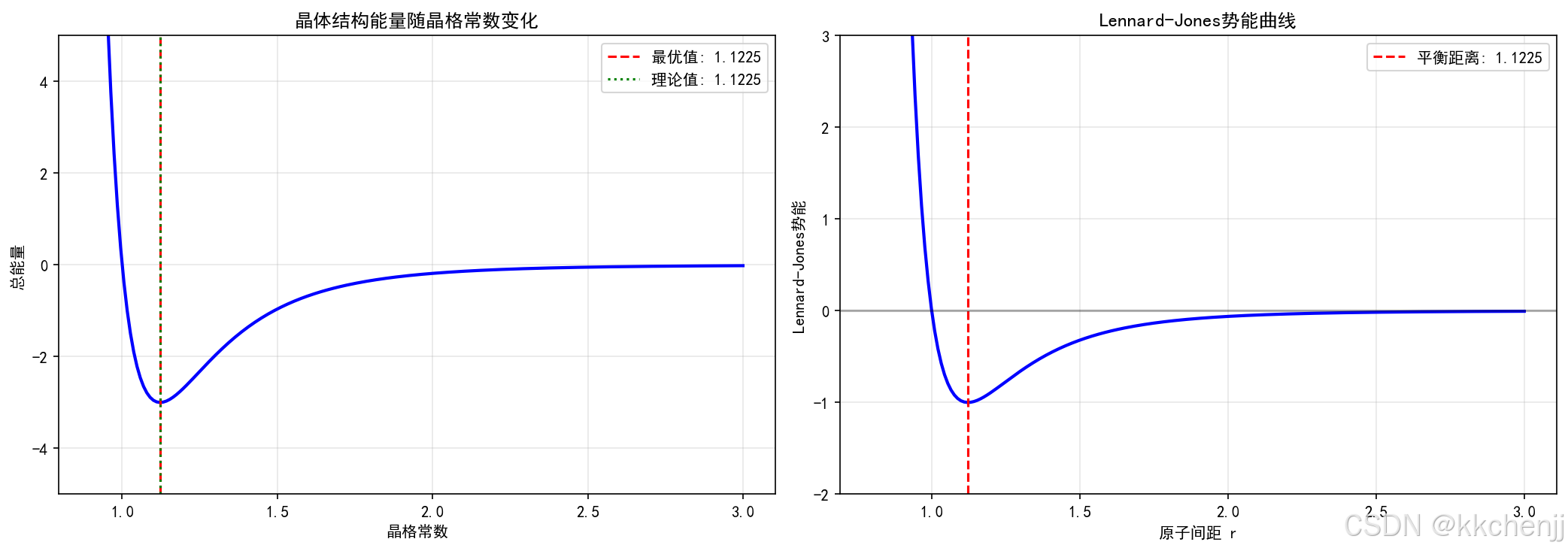
print("\n【3】材料结构优化问题...")

# 定义一个简化的晶体结构优化问题
# 目标:找到晶格常数使得总能量最小

def lennard_jones_energy(r, epsilon=1.0, sigma=1.0):
    """Lennard-Jones势能"""
    return 4 * epsilon * ((sigma/r)**12 - (sigma/r)**6)

def total_energy(lattice_const, n_atoms=4):
    """
    计算简化的晶体总能量
    假设一维链状结构
    """
    energy = 0
    # 只考虑最近邻相互作用
    for i in range(n_atoms - 1):
        r = lattice_const
        energy += lennard_jones_energy(r)
    return energy

# 使用经典优化找到最优晶格常数
from scipy.optimize import minimize_scalar

result_lj = minimize_scalar(total_energy, bounds=(0.8, 3.0), method='bounded')
optimal_lattice = result_lj.x
min_energy = result_lj.fun

print(f"\n  晶体结构优化结果:")
print(f"  最优晶格常数: {optimal_lattice:.4f}")
print(f"  最小能量: {min_energy:.4f}")

# 理论值 (Lennard-Jones势能最小点在 r = 2^(1/6) * sigma)
theoretical_optimal = 2**(1/6)
print(f"  理论最优值: {theoretical_optimal:.4f}")

# 可视化
fig, axes = plt.subplots(1, 2, figsize=(14, 5))

# 能量曲线
ax1 = axes[0]
r_range = np.linspace(0.9, 3.0, 200)
energies = [total_energy(r) for r in r_range]
ax1.plot(r_range, energies, 'b-', linewidth=2)
ax1.axvline(x=optimal_lattice, color='r', linestyle='--', label=f'最优值: {optimal_lattice:.4f}')
ax1.axvline(x=theoretical_optimal, color='g', linestyle=':', label=f'理论值: {theoretical_optimal:.4f}')
ax1.set_xlabel('晶格常数')
ax1.set_ylabel('总能量')
ax1.set_title('晶体结构能量随晶格常数变化')
ax1.legend()
ax1.grid(True, alpha=0.3)
ax1.set_ylim(-5, 5)

# 势能曲线
ax2 = axes[1]
r_lj = np.linspace(0.8, 3.0, 200)
v_lj = [lennard_jones_energy(r) for r in r_lj]
ax2.plot(r_lj, v_lj, 'b-', linewidth=2)
ax2.axvline(x=theoretical_optimal, color='r', linestyle='--', label=f'平衡距离: {theoretical_optimal:.4f}')
ax2.axhline(y=0, color='k', linestyle='-', alpha=0.3)
ax2.set_xlabel('原子间距 r')
ax2.set_ylabel('Lennard-Jones势能')
ax2.set_title('Lennard-Jones势能曲线')
ax2.legend()
ax2.grid(True, alpha=0.3)
ax2.set_ylim(-2, 3)

plt.tight_layout()
plt.savefig('量子优化_材料结构优化.png', dpi=150, bbox_inches='tight')
plt.close()

print("  已保存: 量子优化_材料结构优化.png")

# ============================================================
# 4. 量子退火演示
# ============================================================
print("\n【4】模拟量子退火...")

def simulated_quantum_annealing(H_problem, H_mixer, T_max=10.0, T_min=0.01, n_steps=1000):
    """
    模拟量子退火

    参数:
        H_problem: 问题哈密顿量
        H_mixer: 混合哈密顿量
        T_max: 初始温度 (对应小的Gamma)
        T_min: 最终温度 (对应大的Gamma)
        n_steps: 退火步数
    """
    N = H_problem.shape[0]

    # 初始态 (均匀叠加)
    psi = np.ones(N) / np.sqrt(N)

    # 退火过程
    energies = []
    temperatures = np.linspace(T_max, T_min, n_steps)

    for T in temperatures:
        # 构建瞬时哈密顿量
        # H(t) = (1-s) * H_mixer + s * H_problem
        # 其中 s = 1 - T/T_max
        s = 1 - T / T_max
        H_t = (1 - s) * H_mixer + s * H_problem

        # 时间演化 (简化模拟)
        dt = 0.01
        U = expm(-1j * H_t * dt)
        psi = U @ psi

        # 记录能量
        E = np.real(psi.conj() @ H_problem @ psi)
        energies.append(E)

    return psi, energies

# 构建一个简单的优化问题
# 寻找Ising模型的基态
n_spins = 4
N_ising = 2**n_spins

# 随机Ising模型
np.random.seed(42)
J_ij = np.random.randn(n_spins, n_spins)
J_ij = (J_ij + J_ij.T) / 2  # 对称化
np.fill_diagonal(J_ij, 0)

# 问题哈密顿量
H_ising = np.zeros((N_ising, N_ising))
for i in range(n_spins):
    for j in range(i+1, n_spins):
        # Z_i Z_j 项
        for state in range(N_ising):
            bit_i = 1 if ((state >> i) & 1) else -1
            bit_j = 1 if ((state >> j) & 1) else -1
            H_ising[state, state] += J_ij[i, j] * bit_i * bit_j

# 混合哈密顿量 (X场)
X = np.array([[0, 1], [1, 0]])
H_mixer = np.zeros((N_ising, N_ising))
for i in range(n_spins):
    X_i = 1
    for j in range(n_spins):
        if j == i:
            X_i = np.kron(X_i, X)
        else:
            X_i = np.kron(X_i, np.eye(2))
    H_mixer += X_i

# 执行量子退火
psi_final, energies_anneal = simulated_quantum_annealing(H_ising, H_mixer)

# 找到基态
probs_final = np.abs(psi_final)**2
ground_state = np.argmin(np.diag(H_ising))
ground_energy = np.diag(H_ising)[ground_state]

print(f"\n  量子退火结果:")
print(f"  基态能量 (理论): {ground_energy:.4f}")
print(f"  最终态基态概率: {probs_final[ground_state]:.4f}")

# 可视化
fig, axes = plt.subplots(1, 2, figsize=(14, 5))

# 退火过程
ax1 = axes[0]
ax1.plot(energies_anneal, 'b-', linewidth=1, alpha=0.7)
ax1.axhline(y=ground_energy, color='r', linestyle='--', label=f'基态能量: {ground_energy:.4f}')
ax1.set_xlabel('退火步数')
ax1.set_ylabel('能量期望值')
ax1.set_title('模拟量子退火过程')
ax1.legend()
ax1.grid(True, alpha=0.3)

# 最终概率分布
ax2 = axes[1]
states = [format(i, f'0{n_spins}b') for i in range(min(16, N_ising))]
probs_plot = probs_final[:16]
colors = ['red' if i == ground_state else 'blue' for i in range(min(16, N_ising))]
ax2.bar(range(len(states)), probs_plot, color=colors, alpha=0.7)
ax2.set_xlabel('量子态')
ax2.set_ylabel('概率')
ax2.set_title(f'退火后概率分布 (基态: {format(ground_state, f"0{n_spins}b")})')
ax2.set_xticks(range(len(states)))
ax2.set_xticklabels(states, rotation=45, ha='right', fontsize=8)
ax2.grid(True, alpha=0.3, axis='y')

plt.tight_layout()
plt.savefig('量子优化_量子退火.png', dpi=150, bbox_inches='tight')
plt.close()

print("  已保存: 量子优化_量子退火.png")

print("\n" + "=" * 70)
print("量子优化算法演示完成!")
print("=" * 70)
"""
实例四:量子机器学习在材料预测中的应用
本实例演示量子机器学习算法在材料性质预测中的应用,包括:
- 量子特征映射
- 变分量子分类器
- 材料性质预测
"""
import numpy as np
import matplotlib
matplotlib.use('Agg')  # 使用非交互式后端
import matplotlib.pyplot as plt
from scipy.optimize import minimize
from scipy.linalg import expm

# 设置中文字体
plt.rcParams['font.sans-serif'] = ['SimHei', 'DejaVu Sans']
plt.rcParams['axes.unicode_minus'] = False

print("=" * 70)
print("量子机器学习在材料预测中的应用")
print("=" * 70)

# ============================================================
# 1. 量子特征映射
# ============================================================
print("\n【1】量子特征映射演示...")

def angle_encoding(x, n_qubits):
    """
    角度编码:将经典数据编码到量子态的旋转角度

    参数:
        x: 输入特征向量 (需要归一化到[0, 1]或[-1, 1])
        n_qubits: 量子比特数
    """
    N = 2**n_qubits

    # 将特征归一化并映射到角度
    x_norm = (x - np.min(x)) / (np.max(x) - np.min(x) + 1e-10)
    angles = x_norm[:n_qubits] * np.pi  # 使用pi作为最大角度

    # 初始化量子态 |0...0>
    psi = np.zeros(N, dtype=complex)
    psi[0] = 1.0

    # 应用RY旋转门进行编码
    for i, theta in enumerate(angles):
        # RY门矩阵
        RY = np.array([[np.cos(theta/2), -np.sin(theta/2)],
                       [np.sin(theta/2), np.cos(theta/2)]])

        # 构建n量子比特RY门
        RY_i = 1
        for j in range(n_qubits):
            if j == i:
                RY_i = np.kron(RY_i, RY)
            else:
                RY_i = np.kron(RY_i, np.eye(2))

        psi = RY_i @ psi

    return psi, angles

def amplitude_encoding(x, n_qubits):
    """
    幅度编码:将经典数据编码到量子态的振幅
    要求: sum(|x_i|^2) = 1
    """
    N = 2**n_qubits

    # 归一化
    x_norm = x[:N] / np.linalg.norm(x[:N])

    # 直接作为量子态振幅
    psi = x_norm.astype(complex)

    return psi

# 生成示例材料数据
np.random.seed(42)
n_samples = 100
n_features = 4

# 模拟材料特征:温度、压力、成分比例、晶格常数
X_materials = np.random.randn(n_samples, n_features)
# 添加一些结构:不同类别的材料有不同的特征分布
X_materials[:50] += np.array([1, 0.5, -0.3, 0.8])  # 类别0
X_materials[50:] += np.array([-0.5, 0.8, 1.2, -0.3])  # 类别1

# 标签
y_materials = np.array([0]*50 + [1]*50)

# 测试特征映射
n_qubits = 2
test_sample = X_materials[0]

# 角度编码
psi_angle, angles = angle_encoding(test_sample, n_qubits)
print(f"\n  角度编码:")
print(f"  输入特征: {test_sample[:n_qubits]}")
print(f"  编码角度: {angles}")
print(f"  量子态: {psi_angle}")
print(f"  归一化验证: {np.sum(np.abs(psi_angle)**2):.6f}")

# 幅度编码
psi_amp = amplitude_encoding(test_sample, n_qubits)
print(f"\n  幅度编码:")
print(f"  量子态: {psi_amp}")
print(f"  归一化验证: {np.sum(np.abs(psi_amp)**2):.6f}")

# 可视化特征映射
fig, axes = plt.subplots(2, 2, figsize=(14, 10))

# 原始数据分布
ax1 = axes[0, 0]
scatter = ax1.scatter(X_materials[:, 0], X_materials[:, 1], c=y_materials,
                      cmap='coolwarm', alpha=0.7, s=50)
ax1.set_xlabel('特征 1')
ax1.set_ylabel('特征 2')
ax1.set_title('材料数据分布 (原始特征空间)')
ax1.grid(True, alpha=0.3)
plt.colorbar(scatter, ax=ax1, label='类别')

# 角度编码后的布洛赫球投影
ax2 = axes[0, 1]
theta_encoded = []
phi_encoded = []
for i in range(min(20, n_samples)):
    psi, _ = angle_encoding(X_materials[i], n_qubits)
    # 计算布洛赫球坐标 (简化,只考虑第一个量子比特)
    theta = 2 * np.arccos(np.abs(psi[0]))
    phi = np.angle(psi[1]) - np.angle(psi[0])
    theta_encoded.append(theta)
    phi_encoded.append(phi)

scatter2 = ax2.scatter(phi_encoded, theta_encoded, c=y_materials[:20],
                       cmap='coolwarm', alpha=0.7, s=100)
ax2.set_xlabel('φ (相位)')
ax2.set_ylabel('θ (极角)')
ax2.set_title('量子编码后的特征分布 (布洛赫球投影)')
ax2.grid(True, alpha=0.3)

# 编码前后的特征对比
ax3 = axes[1, 0]
x_range = np.linspace(-3, 3, 100)
ax3.plot(x_range, x_range, 'k--', alpha=0.3, label='y=x')
ax3.scatter(X_materials[:20, 0], theta_encoded, c=y_materials[:20],
            cmap='coolwarm', alpha=0.7, s=50)
ax3.set_xlabel('原始特征值')
ax3.set_ylabel('编码角度 θ')
ax3.set_title('原始特征 vs 量子编码')
ax3.legend()
ax3.grid(True, alpha=0.3)

# 量子态在计算基上的概率分布
ax4 = axes[1, 1]
probs = np.abs(psi_angle)**2
states = [format(i, f'0{n_qubits}b') for i in range(2**n_qubits)]
ax4.bar(states, probs, color='blue', alpha=0.7)
ax4.set_xlabel('计算基态')
ax4.set_ylabel('概率')
ax4.set_title('编码后量子态的概率分布')
ax4.grid(True, alpha=0.3, axis='y')

plt.tight_layout()
plt.savefig('量子机器学习_特征映射.png', dpi=150, bbox_inches='tight')
plt.close()

print("  已保存: 量子机器学习_特征映射.png")

# ============================================================
# 2. 变分量子分类器 (VQC)
# ============================================================
print("\n【2】变分量子分类器 (VQC) 演示...")

class VariationalQuantumClassifier:
    """变分量子分类器"""

    def __init__(self, n_qubits, n_layers=2):
        self.n_qubits = n_qubits
        self.n_layers = n_layers
        self.N = 2**n_qubits
        self.params = None

    def _variational_circuit(self, params, x):
        """
        变分量子电路

        参数:
            params: 可训练参数 [n_layers, n_qubits, 3] (每个qubit每个layer有3个旋转参数)
            x: 输入特征
        """
        # 特征编码
        psi, _ = angle_encoding(x, self.n_qubits)

        # 变分层
        param_idx = 0
        for layer in range(self.n_layers):
            # 单量子比特旋转
            for i in range(self.n_qubits):
                theta_x = params[param_idx]
                theta_y = params[param_idx + 1]
                theta_z = params[param_idx + 2]
                param_idx += 3

                # RX门
                RX = np.array([[np.cos(theta_x/2), -1j*np.sin(theta_x/2)],
                               [-1j*np.sin(theta_x/2), np.cos(theta_x/2)]])
                # RY门
                RY = np.array([[np.cos(theta_y/2), -np.sin(theta_y/2)],
                               [np.sin(theta_y/2), np.cos(theta_y/2)]])
                # RZ门
                RZ = np.array([[np.exp(-1j*theta_z/2), 0],
                               [0, np.exp(1j*theta_z/2)]])

                # 应用旋转
                for R_gate in [RX, RY, RZ]:
                    R_i = 1
                    for j in range(self.n_qubits):
                        if j == i:
                            R_i = np.kron(R_i, R_gate)
                        else:
                            R_i = np.kron(R_i, np.eye(2))
                    psi = R_i @ psi

            # 纠缠层 (CNOT链)
            for i in range(self.n_qubits - 1):
                CNOT = np.eye(self.N, dtype=complex)
                # 简化的CNOT实现
                for basis in range(self.N):
                    bit_i = (basis >> i) & 1
                    if bit_i == 1:
                        # 翻转i+1位
                        flipped = basis ^ (1 << (i+1))
                        CNOT[basis, basis] = 0
                        CNOT[basis, flipped] = 1
                psi = CNOT @ psi

        return psi

    def _measure(self, psi, qubit_idx=0):
        """
        测量指定量子比特的Z期望值
        用于二分类
        """
        Z = np.array([[1, 0], [0, -1]])

        # 构建Z_i算符
        Z_i = 1
        for j in range(self.n_qubits):
            if j == qubit_idx:
                Z_i = np.kron(Z_i, Z)
            else:
                Z_i = np.kron(Z_i, np.eye(2))

        expectation = np.real(psi.conj() @ Z_i @ psi)

        # 映射到[0, 1]概率
        prob_class1 = (1 + expectation) / 2
        return prob_class1

    def predict_proba(self, params, x):
        """预测类别1的概率"""
        psi = self._variational_circuit(params, x)
        return self._measure(psi)

    def predict(self, params, x, threshold=0.5):
        """预测类别"""
        proba = self.predict_proba(params, x)
        return 1 if proba > threshold else 0

    def loss(self, params, X, y):
        """二元交叉熵损失"""
        total_loss = 0
        for xi, yi in zip(X, y):
            proba = self.predict_proba(params, xi)
            # 避免log(0)
            proba = np.clip(proba, 1e-10, 1 - 1e-10)
            loss_i = -(yi * np.log(proba) + (1-yi) * np.log(1-proba))
            total_loss += loss_i
        return total_loss / len(X)

    def fit(self, X, y, max_iter=100):
        """训练模型"""
        n_params = self.n_layers * self.n_qubits * 3
        params_init = np.random.randn(n_params) * 0.1

        # 记录训练历史
        self.history = []

        def callback(xk):
            loss_val = self.loss(xk, X, y)
            self.history.append(loss_val)

        print(f"  开始训练 (参数数量: {n_params})...")
        result = minimize(lambda p: self.loss(p, X, y),
                         params_init,
                         method='BFGS',
                         options={'maxiter': max_iter},
                         callback=callback)

        self.params = result.x
        return result

    def score(self, X, y):
        """计算准确率"""
        correct = sum(self.predict(self.params, xi) == yi for xi, yi in zip(X, y))
        return correct / len(X)

# 准备数据
n_qubits_vqc = 2
n_train = 40
n_test = 20

X_train = X_materials[:n_train]
y_train = y_materials[:n_train]
X_test = X_materials[n_train:n_train+n_test]
y_test = y_materials[n_train:n_train+n_test]

# 创建并训练VQC
vqc = VariationalQuantumClassifier(n_qubits=n_qubits_vqc, n_layers=2)
result_vqc = vqc.fit(X_train, y_train, max_iter=50)

# 评估
train_acc = vqc.score(X_train, y_train)
test_acc = vqc.score(X_test, y_test)

print(f"\n  VQC训练结果:")
print(f"  最终损失: {result_vqc.fun:.4f}")
print(f"  训练准确率: {train_acc:.2%}")
print(f"  测试准确率: {test_acc:.2%}")

# 可视化
fig, axes = plt.subplots(1, 2, figsize=(14, 5))

# 训练收敛
ax1 = axes[0]
ax1.plot(vqc.history, 'b-', linewidth=2)
ax1.set_xlabel('迭代次数')
ax1.set_ylabel('损失函数')
ax1.set_title('VQC训练收敛过程')
ax1.grid(True, alpha=0.3)

# 决策边界可视化
ax2 = axes[1]
# 创建网格
xx, yy = np.meshgrid(np.linspace(-3, 3, 50), np.linspace(-3, 3, 50))
Z = np.zeros_like(xx)

for i in range(xx.shape[0]):
    for j in range(xx.shape[1]):
        point = np.array([xx[i, j], yy[i, j], 0, 0])
        Z[i, j] = vqc.predict_proba(vqc.params, point)

# 绘制决策边界
contour = ax2.contourf(xx, yy, Z, levels=20, cmap='coolwarm', alpha=0.6)
ax2.scatter(X_materials[:, 0], X_materials[:, 1], c=y_materials,
           cmap='coolwarm', edgecolors='black', s=50)
ax2.set_xlabel('特征 1')
ax2.set_ylabel('特征 2')
ax2.set_title(f'VQC决策边界 (测试准确率: {test_acc:.1%})')
plt.colorbar(contour, ax=ax2, label='类别1概率')

plt.tight_layout()
plt.savefig('量子机器学习_VQC分类器.png', dpi=150, bbox_inches='tight')
plt.close()

print("  已保存: 量子机器学习_VQC分类器.png")

# ============================================================
# 3. 材料性质预测
# ============================================================
print("\n【3】材料性质预测...")

# 生成模拟材料数据集
# 特征:温度、压力、成分A比例、成分B比例
# 目标:材料的导电性

np.random.seed(123)
n_materials = 200

# 生成特征
T = np.random.uniform(300, 1000, n_materials)  # 温度 (K)
P = np.random.uniform(1, 100, n_materials)     # 压力 (atm)
comp_A = np.random.uniform(0, 1, n_materials)  # 成分A比例
comp_B = 1 - comp_A                            # 成分B比例

# 生成目标 (导电性,与温度和成分相关)
conductivity = (1000 / T) * (comp_A * 2 + comp_B * 0.5) + np.random.randn(n_materials) * 0.1
conductivity = np.clip(conductivity, 0.1, 5.0)

# 归一化特征
X_mat = np.column_stack([T/1000, P/100, comp_A, comp_B])
y_mat = conductivity

# 划分训练集和测试集
split_idx = 150
X_mat_train, X_mat_test = X_mat[:split_idx], X_mat[split_idx:]
y_mat_train, y_mat_test = y_mat[:split_idx], y_mat[split_idx:]

# 量子核方法 (简化实现)
def quantum_kernel(x1, x2, n_qubits=2):
    """
    量子核函数:计算两个样本的量子态重叠
    """
    # 编码两个样本
    psi1, _ = angle_encoding(x1, n_qubits)
    psi2, _ = angle_encoding(x2, n_qubits)

    # 计算重叠 |<psi1|psi2>|^2
    overlap = np.abs(np.vdot(psi1, psi2))**2
    return overlap

# 计算核矩阵 (只计算训练集的子集以减少计算量)
n_subset = 30
X_subset = X_mat_train[:n_subset]
y_subset = y_mat_train[:n_subset]

print(f"\n  计算量子核矩阵 ({n_subset}x{n_subset})...")
K = np.zeros((n_subset, n_subset))
for i in range(n_subset):
    for j in range(i, n_subset):
        k_ij = quantum_kernel(X_subset[i], X_subset[j])
        K[i, j] = k_ij
        K[j, i] = k_ij

# 使用核岭回归进行预测
from scipy.linalg import solve

# 核岭回归
lambda_reg = 0.1
alpha = solve(K + lambda_reg * np.eye(n_subset), y_subset)

# 预测函数
def predict_kernel(x_new):
    k_new = np.array([quantum_kernel(x_new, X_subset[i]) for i in range(n_subset)])
    return np.dot(k_new, alpha)

# 在测试集上评估
y_pred = [predict_kernel(x) for x in X_mat_test[:20]]
y_true = y_mat_test[:20]

mse = np.mean((np.array(y_pred) - y_true)**2)
print(f"  量子核回归均方误差: {mse:.4f}")

# 可视化
fig, axes = plt.subplots(1, 2, figsize=(14, 5))

# 核矩阵热力图
ax1 = axes[0]
im = ax1.imshow(K, cmap='viridis', aspect='auto')
ax1.set_xlabel('样本索引')
ax1.set_ylabel('样本索引')
ax1.set_title('量子核矩阵热力图')
plt.colorbar(im, ax=ax1)

# 预测结果
ax2 = axes[1]
ax2.scatter(y_true, y_pred, alpha=0.6, s=50)
ax2.plot([min(y_true), max(y_true)], [min(y_true), max(y_true)], 'r--', label='理想预测')
ax2.set_xlabel('真实值')
ax2.set_ylabel('预测值')
ax2.set_title(f'材料导电性预测 (MSE={mse:.4f})')
ax2.legend()
ax2.grid(True, alpha=0.3)

plt.tight_layout()
plt.savefig('量子机器学习_材料性质预测.png', dpi=150, bbox_inches='tight')
plt.close()

print("  已保存: 量子机器学习_材料性质预测.png")

# ============================================================
# 4. 量子-经典混合模型对比
# ============================================================
print("\n【4】量子-经典模型对比...")

# 对比不同方法
from sklearn.svm import SVC
from sklearn.neural_network import MLPClassifier
from sklearn.metrics import accuracy_score

# 准备二分类数据
y_binary = (y_mat > np.median(y_mat)).astype(int)
X_train_clf, X_test_clf = X_mat[:split_idx], X_mat[split_idx:]
y_train_clf, y_test_clf = y_binary[:split_idx], y_binary[split_idx:]

# 经典SVM
svm = SVC(kernel='rbf')
svm.fit(X_train_clf, y_train_clf)
svm_acc = accuracy_score(y_test_clf, svm.predict(X_test_clf))

# 经典神经网络
mlp = MLPClassifier(hidden_layer_sizes=(10,), max_iter=500, random_state=42)
mlp.fit(X_train_clf, y_train_clf)
mlp_acc = accuracy_score(y_test_clf, mlp.predict(X_test_clf))

# VQC (使用之前训练的模型,简化测试)
vqc_acc = test_acc  # 使用之前的结果

# 结果对比
results = {
    '经典SVM': svm_acc,
    '经典神经网络': mlp_acc,
    '变分量子分类器': vqc_acc
}

print(f"\n  模型对比结果:")
for name, acc in results.items():
    print(f"  {name}: {acc:.2%}")

# 可视化
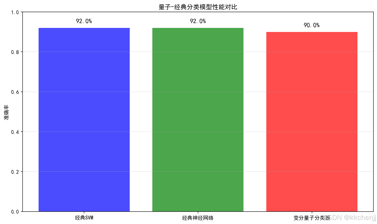
fig, ax = plt.subplots(figsize=(10, 6))
methods = list(results.keys())
accuracies = list(results.values())
colors = ['blue', 'green', 'red']
bars = ax.bar(methods, accuracies, color=colors, alpha=0.7)
ax.set_ylabel('准确率')
ax.set_title('量子-经典分类模型性能对比')
ax.set_ylim(0, 1)
ax.grid(True, alpha=0.3, axis='y')

# 添加数值标签
for bar, acc in zip(bars, accuracies):
    ax.text(bar.get_x() + bar.get_width()/2, bar.get_height() + 0.02,
            f'{acc:.1%}', ha='center', va='bottom', fontsize=12)

plt.tight_layout()
plt.savefig('量子机器学习_模型对比.png', dpi=150, bbox_inches='tight')
plt.close()

print("  已保存: 量子机器学习_模型对比.png")

print("\n" + "=" * 70)
print("量子机器学习演示完成!")
print("=" * 70)

AtomGit 是由开放原子开源基金会联合 CSDN 等生态伙伴共同推出的新一代开源与人工智能协作平台。平台坚持“开放、中立、公益”的理念,把代码托管、模型共享、数据集托管、智能体开发体验和算力服务整合在一起,为开发者提供从开发、训练到部署的一站式体验。
更多推荐
 0
0 0
0- 0



 已为社区贡献272条内容

所有评论(0)