主题042：不确定性量化与可靠性分析

目录

1. 引言
2. 不确定性来源与分类
3. 蒙特卡洛方法
4. 可靠性分析基础
5. 敏感性分析
6. 代理模型方法
7. 工程应用案例
8. 总结与展望

---

1. 引言

1.1 为什么需要不确定性量化

在工程实践中，热应力仿真面临诸多不确定性因素：

材料参数不确定性：材料的热导率、弹性模量、热膨胀系数等物理参数存在批次差异和测量误差。

边界条件不确定性：实际工作环境中的温度、热流密度、对流系数往往难以精确确定。

几何不确定性：制造公差导致实际结构尺寸与设计值存在偏差。

模型不确定性：数学模型对物理过程的简化引入的误差。

传统确定性分析给出单一结果，无法反映这些不确定性的影响。不确定性量化（Uncertainty Quantification, UQ）和可靠性分析为工程决策提供更全面的风险评估。

1.2 本主题学习目标

通过本主题的学习，读者将能够：

1. 识别不确定性来源：理解工程中各类不确定性的本质和特征
2. 掌握蒙特卡洛方法：实现基于随机抽样的不确定性传播分析
3. 进行可靠性评估：计算失效概率和可靠度指数
4. 开展敏感性分析：识别对输出影响最大的输入参数
5. 应用代理模型：提高大规模不确定性分析的计算效率

---

2. 不确定性来源与分类

2.1 随机不确定性（偶然不确定性）

定义：由自然变异引起，不可通过增加知识消除。

典型来源：

• 材料属性的批次差异
• 环境条件的随机波动
• 制造过程的固有变异

数学描述：使用概率分布（正态分布、对数正态分布、威布尔分布等）

2.2 认知不确定性（系统不确定性）

定义：由知识不足引起，可通过增加信息减少。

典型来源：

• 模型简化假设
• 参数测量误差
• 边界条件估计偏差

数学描述：可使用概率方法或区间分析、模糊理论等

2.3 不确定性传播

输入不确定性通过模型传播到输出：

$$Y=f(X_1,X_2,...,X_n)$$

其中 $X_i$ 是随机输入变量，$Y$ 是随机输出变量。

---

3. 蒙特卡洛方法

3.1 基本原理

蒙特卡洛方法通过随机抽样估计数学问题的数值解。核心思想是：用频率估计概率。

算法流程：

1. 定义输入随机变量的概率分布
2. 生成N组随机样本
3. 对每组样本运行确定性模型
4. 统计分析输出结果

3.2 随机数生成

3.2.1 伪随机数

计算机使用确定性算法生成伪随机数序列。常用算法：

• 线性同余法（LCG）
• Mersenne Twister（Python默认）

3.2.2 常用概率分布

正态分布：
$$f(x)=\frac{1}{\sigma \sqrt{2\pi }}\exp \left(-\frac{(x-\mu {)}^2}{2{\sigma }^2}\right)$$

适用于：材料参数、尺寸公差等对称分布的变量。

对数正态分布：
若 $\ln (X)\sim N(\mu ,{\sigma }^2)$，则 $X$ 服从对数正态分布。

适用于：必须为正且右偏的变量，如疲劳寿命、粗糙度。

均匀分布：
$$f(x)=\frac{1}{b-a},x\in [a,b]$$

适用于：仅知道取值范围的变量。

3.3 统计量计算

3.3.1 样本统计量

样本均值：
$$\bar{Y}=\frac{1}{N}\sum _{i=1}^N{Y}_i$$

样本方差：
$$S^2=\frac{1}{N-1}\sum _{i=1}^N(Y_i-\bar{Y}{)}^2$$

变异系数：
$$CoV=\frac{S}{\bar{Y}}$$

3.3.2 分位数估计

$p$ 分位数 ${\hat{y}}_p$ 满足：
$$P(Y\le {\hat{y}}_p)=p$$

蒙特卡洛估计：将样本排序，取第 $[Np]$ 个值。

3.4 收敛性分析

蒙特卡洛方法的误差：
$$ϵ\propto \frac{1}{\sqrt{N}}$$

这意味着：样本量增加100倍，精度提高10倍。

样本量选择：

• 粗略估计：$N=10^3\sim 10^4$
• 精确估计：$N=10^5\sim 10^6$
• 小失效概率：$N=10^6$ 以上

3.5 重要性抽样

对于小失效概率问题，标准蒙特卡洛效率低下。重要性抽样通过改变抽样分布提高效率。

原理：
$$P_f=\int I(g(x)<0)f_X(x)dx=\int I(g(x)<0)\frac{f_X(x)}{h_X(x)}{h}_X(x)dx$$

其中 $h_X(x)$ 是重要性抽样密度，通常选择使失效区域概率增大的分布。

---

4. 可靠性分析基础

4.1 失效概率定义

失效概率：
$$P_f=P(g(X)\le 0)={\int }_{g(x)\le 0}{f}_X(x)dx$$

其中 $g(X)$ 是极限状态函数：

• $g(X)>0$：安全状态
• $g(X)=0$：极限状态
• $g(X)<0$：失效状态

4.2 可靠度指数

一次二阶矩法（FOSM）：

假设 $g(X)$ 服从正态分布，可靠度指数：
$$\beta =\frac{{\mu }_g}{{\sigma }_g}$$

失效概率近似：
$$P_f\approx \Phi (-\beta )$$

其中 $\Phi$ 是标准正态分布函数。

设计点：

标准正态空间中最接近原点的失效面上的点，对应最可能的失效模式。

4.3 蒙特卡洛可靠性分析

直接估计失效概率：
$${\hat{P}}_f=\frac{1}{N}\sum _{i=1}^{N}I(g(X_i)\le 0)$$

其中 $I(\cdot )$ 是指示函数。

方差估计：
$$Var({\hat{P}}_f)=\frac{P_f(1-P_f)}{N}$$

---

5. 敏感性分析

5.1 相关性分析

Pearson相关系数：
$${\rho }_{XY}=\frac{Cov(X,Y)}{{\sigma }_X{\sigma }_Y}$$

取值范围 $[-1,1]$，绝对值越大表示线性相关性越强。

5.2 方差分解

Sobol指数：量化各输入参数对输出方差的贡献。

一阶Sobol指数：
$$S_i=\frac{Va{r}_{X_i}(E_{X_{-i}}[Y|X_i])}{Var(Y)}$$

总效应指数：
$$S_{Ti}=1-\frac{Va{r}_{X_{-i}}(E_{X_i}[Y|X_{-i}])}{Var(Y)}$$

5.3 tornado图

通过改变单个参数（保持其他参数不变），观察输出的变化范围，直观展示参数重要性。

---

6. 代理模型方法

6.1 为什么需要代理模型

复杂工程模型的计算成本高，难以直接用于大规模蒙特卡洛模拟。代理模型（Surrogate Model）提供廉价近似。

6.2 常用代理模型

6.2.1 多项式混沌展开（PCE）

$$Y(\xi )=\sum _{\alpha }{c}_{\alpha }{\Psi }_{\alpha }(\xi )$$

其中 ${\Psi }_{\alpha }$ 是正交多项式，$\xi$ 是标准随机变量。

6.2.2 Kriging模型

基于高斯过程的插值方法：
$$\hat{y}(x)=\mu +Z(x)$$

其中 $Z(x)$ 是均值为0的高斯随机过程。

6.2.3 神经网络

多层感知机作为通用函数逼近器：
$$\hat{y}=f_{NN}(x;\theta )$$

6.3 代理模型验证

留一法交叉验证：
$$Q^2=1-\frac{\sum (y_i-{\hat{y}}_{-i}{)}^2}{\sum (y_i-\bar{y}{)}^2}$$

$Q^2$ 接近1表示代理模型精度高。

---

7. 工程应用案例

7.1 涡轮叶片热应力可靠性分析

问题描述：

• 材料：镍基高温合金
• 不确定性：温度场、材料参数、冷却效率
• 失效模式：热疲劳裂纹

分析流程：

1. 建立参数化热-结构耦合模型
2. 定义输入参数的概率分布
3. 蒙特卡洛模拟（10^5样本）
4. 计算疲劳寿命的失效概率
5. 识别关键敏感参数

7.2 核反应堆压力容器完整性评估

问题描述：

• 瞬态热冲击过程
• 材料断裂韧性不确定性
• 缺陷尺寸分布

分析要点：

• 考虑中子辐照脆化效应
• 采用重要性抽样提高效率
• 评估不同运行工况的失效风险

7.3 电子器件热设计优化

问题描述：

• 多芯片模块的热管理
• 散热器性能变异
• 环境温度波动

优化目标：

• 在满足可靠性约束下最小化成本
• 使用代理模型加速优化

---

8. 总结与展望

8.1 本主题要点回顾

1. 不确定性分类：区分随机不确定性和认知不确定性
2. 蒙特卡洛方法：掌握随机抽样和统计分析方法
3. 可靠性指标：理解失效概率和可靠度指数
4. 敏感性分析：识别关键不确定性来源
5. 代理模型：提高大规模分析的计算效率

8.2 进阶方向

1. 贝叶斯方法：结合先验知识和观测数据更新不确定性
2. 区间分析：处理认知不确定性的非概率方法
3. 多保真度方法：结合高低精度模型提高效率
4. 深度学习：利用神经网络进行不确定性传播
5. 实时不确定性量化：数字孪生中的在线UQ

8.3 软件工具

• Python：UQpy、SALib、Chaospy
• MATLAB：UQLab、Sensitivity Analysis Toolbox
• 商业软件：ANSYS Probabilistic Design, OptiSLang

---

附录：Python代码清单

A.1 蒙特卡洛模拟

"""
主题042：不确定性量化与可靠性分析
实例一：蒙特卡洛模拟

本实例介绍蒙特卡洛方法在热应力不确定性分析中的应用。
"""

import numpy as np
import matplotlib.pyplot as plt
from scipy import stats
from scipy.integrate import odeint

# 设置中文字体
plt.rcParams['font.sans-serif'] = ['SimHei', 'DejaVu Sans']
plt.rcParams['axes.unicode_minus'] = False


def thermal_stress_model(params):
    """
    简化的热应力模型
    
    参数:
    params: [E, alpha, k, q, h] - 弹性模量、热膨胀系数、热导率、热流、对流系数
    
    返回:
    sigma_max: 最大热应力
    """
    E, alpha, k, q, h = params
    
    # 简化的热应力计算
    # 假设温度梯度与热流成正比
    delta_T = q / h  # 特征温差
    sigma_max = E * alpha * delta_T
    
    return sigma_max


def monte_carlo_simulation(n_samples, distributions):
    """
    蒙特卡洛模拟
    
    参数:
    n_samples: 样本数量
    distributions: 参数字典 {name: (dist_type, params)}
    
    返回:
    samples: 输入参数样本 (n_samples, n_params)
    outputs: 输出结果 (n_samples,)
    """
    n_params = len(distributions)
    samples = np.zeros((n_samples, n_params))
    
    # 生成随机样本
    param_names = list(distributions.keys())
    for i, name in enumerate(param_names):
        dist_type, params = distributions[name]
        if dist_type == 'normal':
            samples[:, i] = np.random.normal(params[0], params[1], n_samples)
        elif dist_type == 'uniform':
            samples[:, i] = np.random.uniform(params[0], params[1], n_samples)
        elif dist_type == 'lognormal':
            samples[:, i] = np.random.lognormal(params[0], params[1], n_samples)
    
    # 计算输出
    outputs = np.array([thermal_stress_model(samples[i]) for i in range(n_samples)])
    
    return samples, outputs


def calculate_statistics(outputs):
    """计算统计量"""
    stats_dict = {
        'mean': np.mean(outputs),
        'std': np.std(outputs),
        'cov': np.std(outputs) / np.mean(outputs),
        'min': np.min(outputs),
        'max': np.max(outputs),
        'median': np.median(outputs),
        'p5': np.percentile(outputs, 5),
        'p95': np.percentile(outputs, 95)
    }
    return stats_dict


def reliability_analysis(outputs, threshold):
    """
    可靠性分析
    
    参数:
    outputs: 输出样本
    threshold: 失效阈值
    
    返回:
    pf: 失效概率
    beta: 可靠度指数
    """
    n_fail = np.sum(outputs > threshold)
    pf = n_fail / len(outputs)
    
    # 可靠度指数 (假设正态分布)
    mu = np.mean(outputs)
    sigma = np.std(outputs)
    beta = (threshold - mu) / sigma
    
    return pf, beta


def example_1_basic_mc():
    """示例1：基础蒙特卡洛模拟"""
    
    print("=" * 70)
    print("示例1：基础蒙特卡洛模拟")
    print("=" * 70)
    
    # 定义输入参数分布
    distributions = {
        'E': ('normal', (200e9, 10e9)),      # 弹性模量 (Pa)
        'alpha': ('normal', (12e-6, 0.5e-6)), # 热膨胀系数 (1/K)
        'k': ('uniform', (40, 60)),           # 热导率 (W/m·K)
        'q': ('normal', (1e6, 0.1e6)),        # 热流 (W/m²)
        'h': ('lognormal', (np.log(100), 0.1)) # 对流系数 (W/m²·K)
    }
    
    # 运行蒙特卡洛模拟
    n_samples = 10000
    samples, outputs = monte_carlo_simulation(n_samples, distributions)
    
    # 计算统计量
    stats = calculate_statistics(outputs)
    
    print(f"\n样本数量: {n_samples}")
    print(f"\n热应力统计结果:")
    print(f"  均值: {stats['mean']/1e6:.2f} MPa")
    print(f"  标准差: {stats['std']/1e6:.2f} MPa")
    print(f"  变异系数: {stats['cov']*100:.2f}%")
    print(f"  最小值: {stats['min']/1e6:.2f} MPa")
    print(f"  最大值: {stats['max']/1e6:.2f} MPa")
    print(f"  中位数: {stats['median']/1e6:.2f} MPa")
    print(f"  5%分位数: {stats['p5']/1e6:.2f} MPa")
    print(f"  95%分位数: {stats['p95']/1e6:.2f} MPa")
    
    # 可靠性分析
    threshold = 300e6  # 失效阈值 300 MPa
    pf, beta = reliability_analysis(outputs, threshold)
    
    print(f"\n可靠性分析 (阈值={threshold/1e6:.0f} MPa):")
    print(f"  失效概率 Pf = {pf:.6f}")
    print(f"  可靠度指数 β = {beta:.2f}")
    
    # 可视化
    fig, axes = plt.subplots(2, 2, figsize=(12, 10))
    
    # 1. 热应力分布直方图
    ax1 = axes[0, 0]
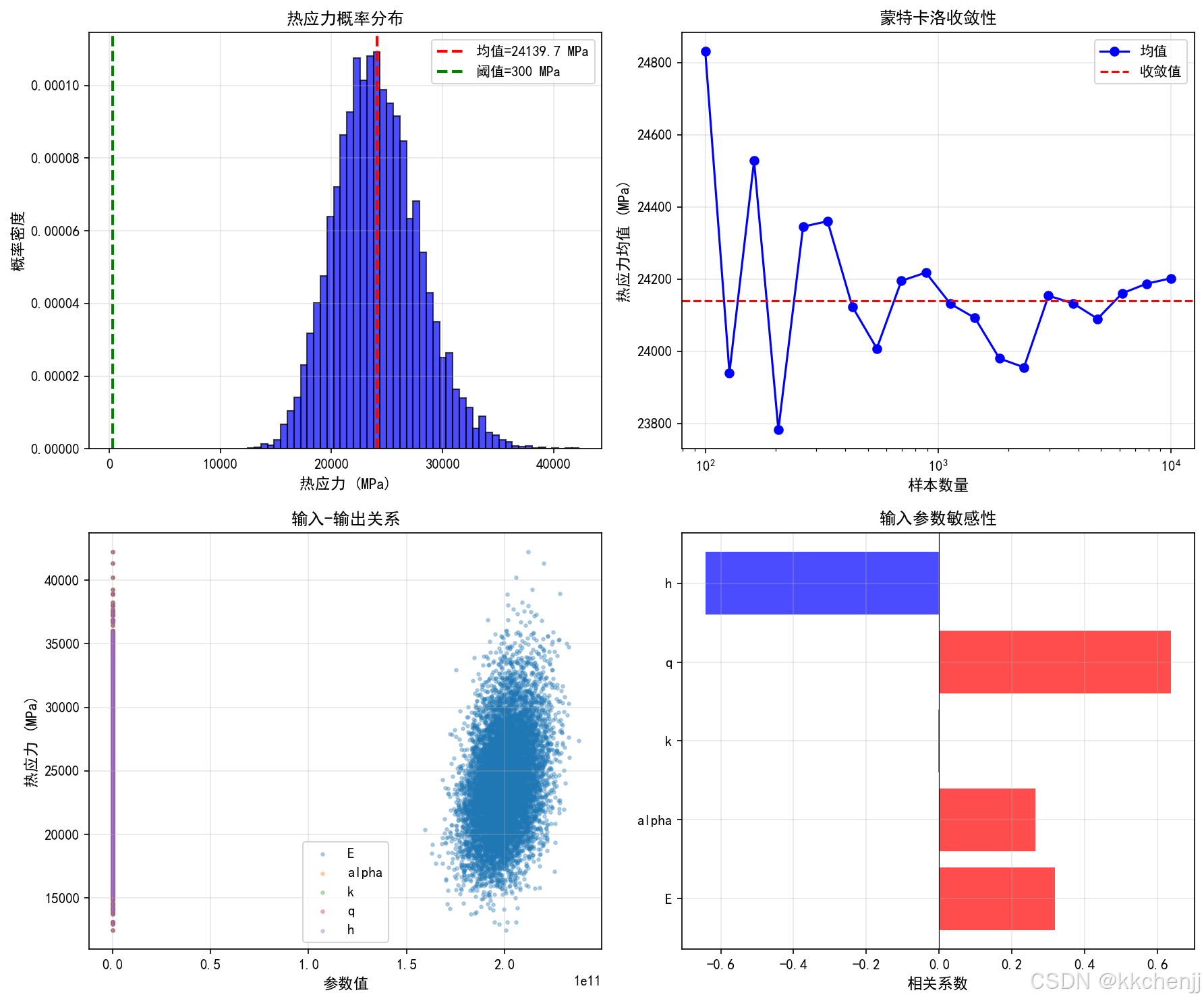
    ax1.hist(outputs/1e6, bins=50, density=True, alpha=0.7, color='blue', edgecolor='black')
    ax1.axvline(stats['mean']/1e6, color='red', linestyle='--', linewidth=2, label=f'均值={stats["mean"]/1e6:.1f} MPa')
    ax1.axvline(threshold/1e6, color='green', linestyle='--', linewidth=2, label=f'阈值={threshold/1e6:.0f} MPa')
    ax1.set_xlabel('热应力 (MPa)', fontsize=11)
    ax1.set_ylabel('概率密度', fontsize=11)
    ax1.set_title('热应力概率分布', fontsize=12, fontweight='bold')
    ax1.legend()
    ax1.grid(True, alpha=0.3)
    
    # 2. 收敛性分析
    ax2 = axes[0, 1]
    sample_sizes = np.logspace(2, 4, 20).astype(int)
    means = []
    stds = []
    
    for n in sample_sizes:
        _, outputs_subset = monte_carlo_simulation(n, distributions)
        means.append(np.mean(outputs_subset))
        stds.append(np.std(outputs_subset))
    
    ax2.semilogx(sample_sizes, np.array(means)/1e6, 'b-o', label='均值')
    ax2.axhline(stats['mean']/1e6, color='red', linestyle='--', label='收敛值')
    ax2.set_xlabel('样本数量', fontsize=11)
    ax2.set_ylabel('热应力均值 (MPa)', fontsize=11)
    ax2.set_title('蒙特卡洛收敛性', fontsize=12, fontweight='bold')
    ax2.legend()
    ax2.grid(True, alpha=0.3)
    
    # 3. 参数敏感性（散点图）
    ax3 = axes[1, 0]
    param_names = list(distributions.keys())
    for i, name in enumerate(param_names):
        ax3.scatter(samples[:, i], outputs/1e6, alpha=0.3, s=5, label=name)
    ax3.set_xlabel('参数值', fontsize=11)
    ax3.set_ylabel('热应力 (MPa)', fontsize=11)
    ax3.set_title('输入-输出关系', fontsize=12, fontweight='bold')
    ax3.legend()
    ax3.grid(True, alpha=0.3)
    
    # 4. 相关系数
    ax4 = axes[1, 1]
    correlations = []
    for i in range(len(param_names)):
        corr = np.corrcoef(samples[:, i], outputs)[0, 1]
        correlations.append(corr)
    
    colors = ['red' if c > 0 else 'blue' for c in correlations]
    ax4.barh(param_names, correlations, color=colors, alpha=0.7)
    ax4.set_xlabel('相关系数', fontsize=11)
    ax4.set_title('输入参数敏感性', fontsize=12, fontweight='bold')
    ax4.axvline(0, color='black', linewidth=0.5)
    ax4.grid(True, alpha=0.3)
    
    plt.tight_layout()
    plt.savefig('mc_basic_analysis.png', dpi=150, bbox_inches='tight')
    print("\n✓ 已保存: mc_basic_analysis.png")
    plt.close()


def example_2_sample_size_effect():
    """示例2：样本数量对结果的影响"""
    
    print("\n" + "=" * 70)
    print("示例2：样本数量对蒙特卡洛结果的影响")
    print("=" * 70)
    
    distributions = {
        'E': ('normal', (200e9, 10e9)),
        'alpha': ('normal', (12e-6, 0.5e-6)),
        'k': ('uniform', (40, 60)),
        'q': ('normal', (1e6, 0.1e6)),
        'h': ('lognormal', (np.log(100), 0.1))
    }
    
    sample_sizes = [100, 500, 1000, 5000, 10000, 50000]
    
    results = []
    for n in sample_sizes:
        samples, outputs = monte_carlo_simulation(n, distributions)
        stats = calculate_statistics(outputs)
        pf, beta = reliability_analysis(outputs, 300e6)
        results.append({
            'n': n,
            'mean': stats['mean'],
            'std': stats['std'],
            'pf': pf,
            'beta': beta
        })
        print(f"n={n:6d}: 均值={stats['mean']/1e6:.2f} MPa, 失效概率={pf:.6f}")
    
    # 可视化
    fig, axes = plt.subplots(1, 2, figsize=(12, 4))
    
    means = [r['mean']/1e6 for r in results]
    stds = [r['std']/1e6 for r in results]
    pfs = [r['pf'] for r in results]
    
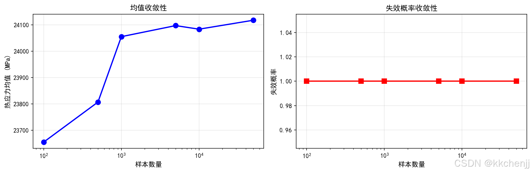
    axes[0].semilogx(sample_sizes, means, 'b-o', linewidth=2, markersize=8)
    axes[0].set_xlabel('样本数量', fontsize=11)
    axes[0].set_ylabel('热应力均值 (MPa)', fontsize=11)
    axes[0].set_title('均值收敛性', fontsize=12, fontweight='bold')
    axes[0].grid(True, alpha=0.3)
    
    axes[1].semilogx(sample_sizes, pfs, 'r-s', linewidth=2, markersize=8)
    axes[1].set_xlabel('样本数量', fontsize=11)
    axes[1].set_ylabel('失效概率', fontsize=11)
    axes[1].set_title('失效概率收敛性', fontsize=12, fontweight='bold')
    axes[1].grid(True, alpha=0.3)
    
    plt.tight_layout()
    plt.savefig('mc_sample_size_effect.png', dpi=150, bbox_inches='tight')
    print("\n✓ 已保存: mc_sample_size_effect.png")
    plt.close()


def example_3_importance_sampling():
    """示例3：重要性抽样"""
    
    print("\n" + "=" * 70)
    print("示例3：重要性抽样方法")
    print("=" * 70)
    
    # 定义原始分布
    mu_E, sigma_E = 200e9, 10e9
    
    # 标准蒙特卡洛
    n_samples = 10000
    E_samples = np.random.normal(mu_E, sigma_E, n_samples)
    
    # 计算热应力 (简化模型)
    sigma_samples = 0.5 * E_samples * 12e-6 * 100  # 假设其他参数固定
    
    # 失效阈值 (高应力区域)
    threshold = 130e6
    
    # 标准MC估计
    pf_mc = np.sum(sigma_samples > threshold) / n_samples
    
    print(f"\n标准蒙特卡洛 (n={n_samples}):")
    print(f"  失效概率估计: {pf_mc:.6f}")
    print(f"  失效样本数: {np.sum(sigma_samples > threshold)}")
    
    # 重要性抽样
    # 将抽样中心移到失效边界附近
    mu_IS = 220e9  # 提高弹性模量均值
    E_samples_IS = np.random.normal(mu_IS, sigma_E, n_samples)
    sigma_samples_IS = 0.5 * E_samples_IS * 12e-6 * 100
    
    # 计算重要性权重
    weights = stats.norm.pdf(E_samples_IS, mu_E, sigma_E) / \
              stats.norm.pdf(E_samples_IS, mu_IS, sigma_E)
    
    # 加权估计失效概率
    pf_is = np.sum((sigma_samples_IS > threshold) * weights) / n_samples
    
    print(f"\n重要性抽样 (n={n_samples}):")
    print(f"  失效概率估计: {pf_is:.6f}")
    print(f"  失效样本数: {np.sum(sigma_samples_IS > threshold)}")
    
    # 可视化
    fig, axes = plt.subplots(1, 2, figsize=(12, 4))
    
    # 原始分布
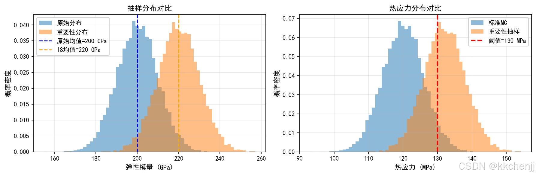
    axes[0].hist(E_samples/1e9, bins=50, density=True, alpha=0.5, label='原始分布')
    axes[0].hist(E_samples_IS/1e9, bins=50, density=True, alpha=0.5, label='重要性分布')
    axes[0].axvline(mu_E/1e9, color='blue', linestyle='--', label=f'原始均值={mu_E/1e9:.0f} GPa')
    axes[0].axvline(mu_IS/1e9, color='orange', linestyle='--', label=f'IS均值={mu_IS/1e9:.0f} GPa')
    axes[0].set_xlabel('弹性模量 (GPa)', fontsize=11)
    axes[0].set_ylabel('概率密度', fontsize=11)
    axes[0].set_title('抽样分布对比', fontsize=12, fontweight='bold')
    axes[0].legend()
    axes[0].grid(True, alpha=0.3)
    
    # 热应力分布
    axes[1].hist(sigma_samples/1e6, bins=50, density=True, alpha=0.5, label='标准MC')
    axes[1].hist(sigma_samples_IS/1e6, bins=50, density=True, alpha=0.5, label='重要性抽样')
    axes[1].axvline(threshold/1e6, color='red', linestyle='--', linewidth=2, label=f'阈值={threshold/1e6:.0f} MPa')
    axes[1].set_xlabel('热应力 (MPa)', fontsize=11)
    axes[1].set_ylabel('概率密度', fontsize=11)
    axes[1].set_title('热应力分布对比', fontsize=12, fontweight='bold')
    axes[1].legend()
    axes[1].grid(True, alpha=0.3)
    
    plt.tight_layout()
    plt.savefig('mc_importance_sampling.png', dpi=150, bbox_inches='tight')
    print("\n✓ 已保存: mc_importance_sampling.png")
    plt.close()


if __name__ == "__main__":
    print("=" * 70)
    print("主题042：不确定性量化与可靠性分析")
    print("实例一：蒙特卡洛模拟")
    print("=" * 70)
    
    # 示例1：基础蒙特卡洛
    example_1_basic_mc()
    
    # 示例2：样本数量影响
    example_2_sample_size_effect()
    
    # 示例3：重要性抽样
    example_3_importance_sampling()
    
    print("\n" + "=" * 70)
    print("实例一完成！")
    print("=" * 70)
    print("\n关键概念:")
    print("1. 蒙特卡洛方法基本原理")
    print("2. 随机抽样与统计量计算")
    print("3. 可靠性分析与失效概率")
    print("4. 收敛性分析与样本数量选择")
    print("5. 重要性抽样提高效率")