主题090_边缘计算中的辐射换热实时模拟
主题090:边缘计算中的辐射换热实时模拟
摘要
随着工业4.0和智能制造的快速发展,辐射换热仿真正从传统的离线计算模式向实时在线模式转变。边缘计算作为一种新兴的计算范式,将计算能力下沉到数据源头,为辐射换热的实时模拟提供了全新的技术路径。本主题系统介绍边缘计算在辐射换热实时模拟中的应用,包括边缘计算架构设计、轻量化模型开发、模型压缩与加速技术、实时数据流处理、以及典型工业场景的解决方案。通过本主题的学习,读者将掌握如何在资源受限的边缘设备上实现高效、准确的辐射换热实时模拟,满足工业现场对低延迟、高可靠性的需求。
关键词
边缘计算、实时模拟、轻量化模型、模型压缩、嵌入式系统、工业物联网、低延迟、辐射换热
1. 引言
1.1 边缘计算的兴起
边缘计算(Edge Computing)是一种分布式计算范式,其核心思想是将计算、存储和网络服务从云端数据中心延伸到网络边缘,靠近数据源和用户。与传统的云计算模式相比,边缘计算具有以下显著优势:
低延迟响应:边缘计算将数据处理放在靠近数据源的位置,避免了数据往返云端的长距离传输,显著降低了响应时间。对于辐射换热实时控制应用,延迟从云端的数百毫秒降低到边缘的数毫秒。
带宽节省:通过在边缘进行数据预处理和过滤,只将关键信息上传到云端,大幅减少网络带宽消耗。在工业炉窑监控场景中,边缘计算可将数据传输量减少90%以上。
隐私保护:敏感数据在本地处理,减少了数据暴露的风险。这对于涉及商业机密的热工过程尤为重要。
离线可用性:即使网络连接中断,边缘设备仍能独立运行,保证关键控制功能的连续性。
可扩展性:边缘节点的分布式部署使得系统可以灵活扩展,适应不同规模的工业应用。
1.2 辐射换热实时模拟的需求
辐射换热在许多工业过程中起着关键作用,实时模拟的需求日益增长:
工业炉窑控制:需要实时监测炉膛温度分布,动态调整燃烧器功率,确保产品质量和能效。延迟超过1秒可能导致温度超标或产品缺陷。
热光伏系统:需要实时追踪太阳位置,调整聚光器和接收器角度,最大化光热转换效率。实时性直接影响系统发电量。
电子器件热管理:芯片温度变化迅速,需要毫秒级的热仿真来预测过热风险,触发保护机制。
建筑能耗管理:根据实时气象数据和室内人员活动,动态调节暖通空调系统,实现节能运行。
航天器热控:在轨运行时,需要根据太阳角度和姿态变化,实时计算温度分布,调整热控策略。
1.3 技术挑战
将辐射换热仿真部署到边缘设备面临诸多挑战:
计算资源受限:边缘设备(如ARM处理器、FPGA、嵌入式GPU)的计算能力和内存容量远不及服务器级CPU/GPU,传统的高精度辐射模型难以直接运行。
实时性要求:工业控制通常要求毫秒级甚至微秒级的响应时间,而辐射换热方程的求解往往需要迭代计算,如何在有限时间内获得足够准确的结果是关键难题。
模型复杂度:辐射传递方程涉及空间、角度和波谱的多维积分,计算复杂度高。在边缘设备上需要开发轻量化的近似模型。
数据同步:边缘设备需要与传感器、执行器和云端进行实时数据交换,如何保证数据一致性和同步性是一个系统工程问题。
可靠性要求:工业环境对系统可靠性要求极高,边缘计算系统需要具备故障检测、自恢复和降级运行能力。
2. 边缘计算架构设计
2.1 系统架构层次
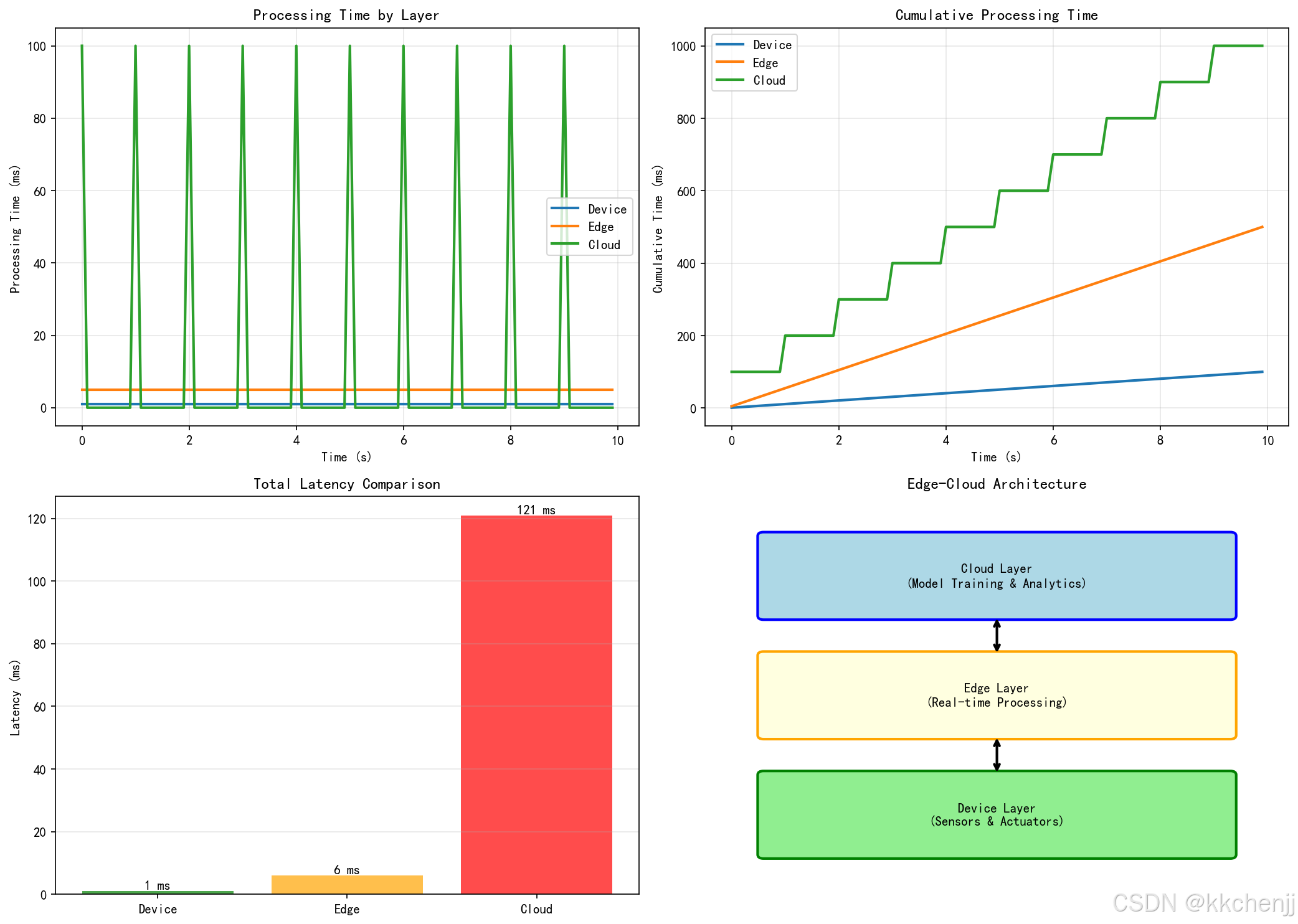
边缘计算系统通常采用三层架构:
云端层(Cloud Layer):负责全局管理、大数据分析、模型训练和长期存储。云端拥有丰富的计算资源,可以运行复杂的辐射模型,生成训练数据,优化轻量化模型。
边缘层(Edge Layer):部署在工厂或现场,负责区域数据聚合、实时处理和本地决策。边缘网关或服务器运行轻量化辐射模型,响应实时控制需求。
设备层(Device Layer):包括传感器、执行器和嵌入式控制器,直接与物理系统交互。这一层进行数据采集和初步处理,执行边缘层下发的控制指令。
在辐射换热应用中,这种分层架构的优势体现在:
- 温度传感器网络将采集数据发送到边缘节点
- 边缘节点运行实时辐射模型,计算温度分布和热流
- 根据计算结果,边缘节点直接控制加热器或冷却系统
- 同时,边缘节点将关键数据上传到云端,用于模型更新和性能分析
2.2 边缘节点硬件平台
边缘计算节点的硬件选择需要权衡计算能力、功耗、成本和可靠性:
ARM处理器:如NVIDIA Jetson系列、Raspberry Pi、NXP i.MX系列。具有低功耗、低成本的优势,适合中低复杂度的辐射模型。Jetson Nano可提供0.5 TFLOPS的AI算力,足以运行小型神经网络模型。
FPGA:现场可编程门阵列,如Xilinx Zynq、Intel Cyclone。FPGA可以定制硬件加速辐射计算的核心算子,实现微秒级响应。适合对延迟要求极高的场景。
嵌入式GPU:如NVIDIA Jetson Xavier、Google Coral。提供强大的并行计算能力,适合运行深度学习加速的辐射模型。Jetson Xavier可提供32 TOPS的AI性能。
ASIC:专用集成电路,为特定辐射模型定制。能效比最高,但开发成本高,灵活性差。适合大规模部署的标准化应用。
2.3 软件架构设计
边缘计算软件架构需要考虑实时性、可靠性和可维护性:
实时操作系统(RTOS):如FreeRTOS、RT-Linux、VxWorks。提供确定性的任务调度和中断响应,保证关键任务的实时执行。
容器化技术:使用Docker或轻量级容器(如balenaEngine)部署应用,实现环境隔离和快速更新。容器化简化了模型部署和版本管理。
微服务架构:将辐射模拟功能拆分为独立的服务模块,如数据采集服务、模型推理服务、控制决策服务。各服务独立开发、部署和扩展。
消息中间件:使用MQTT、Apache Kafka或Redis Streams进行异步消息传递,解耦生产者和消费者,提高系统弹性。
3. 轻量化辐射模型
3.1 模型简化策略
为了在边缘设备上实现实时辐射模拟,需要对传统模型进行简化:
几何简化:将复杂三维几何简化为二维或一维模型。例如,炉膛辐射可以简化为轴对称模型,大幅减少了计算网格数量。
角度离散简化:减少离散坐标法的角度方向数。在边缘设备上,S2或S4离散(4或8个方向)通常已能提供足够的精度。
波谱简化:使用灰体假设或少量灰气体替代全波谱计算。WSGGM模型使用3-4个灰气体组,计算量降低一个数量级。
空间离散简化:采用粗网格或自适应网格细化。在温度梯度小的区域使用大网格,在关键区域使用细网格。
时间步长简化:对于准稳态过程,可以使用较大的时间步长。对于快速瞬态过程,采用隐式格式提高稳定性。
3.2 代理模型方法
代理模型(Surrogate Model)是用简单模型近似复杂仿真的有效方法:
响应面方法(RSM):使用多项式函数拟合辐射换热的输入-输出关系。二次响应面可以在边缘设备上快速计算,适合参数变化范围小的场景。
克里金模型(Kriging):基于高斯过程的插值方法,提供预测的不确定性估计。适合训练数据稀疏的情况,但计算复杂度随数据量增加。
径向基函数网络(RBF):使用径向基函数作为激活函数的神经网络,训练速度快,适合实时更新。
深度神经网络(DNN):使用多层感知机或卷积网络学习辐射场的映射关系。需要离线训练,但推理速度快,精度高。
3.3 降阶模型技术
降阶模型(Reduced-Order Model, ROM)通过提取主要特征降低模型维度:
本征正交分解(POD):对高保真仿真结果进行奇异值分解,提取主导模态。辐射场可以用少量POD模态的线性组合近似。
动态模态分解(DMD):分析辐射场的时空演化,提取动态特征。适合瞬态辐射过程的快速预测。
算子推断(Operator Inference):从仿真数据学习降阶算子,无需访问原始高保真模型。适合黑箱系统的建模。
物理信息神经网络(PINN):将物理约束嵌入神经网络损失函数,提高外推能力和物理一致性。PINN可以在小数据集上训练,适合边缘部署。
4. 模型压缩与加速
4.1 神经网络量化
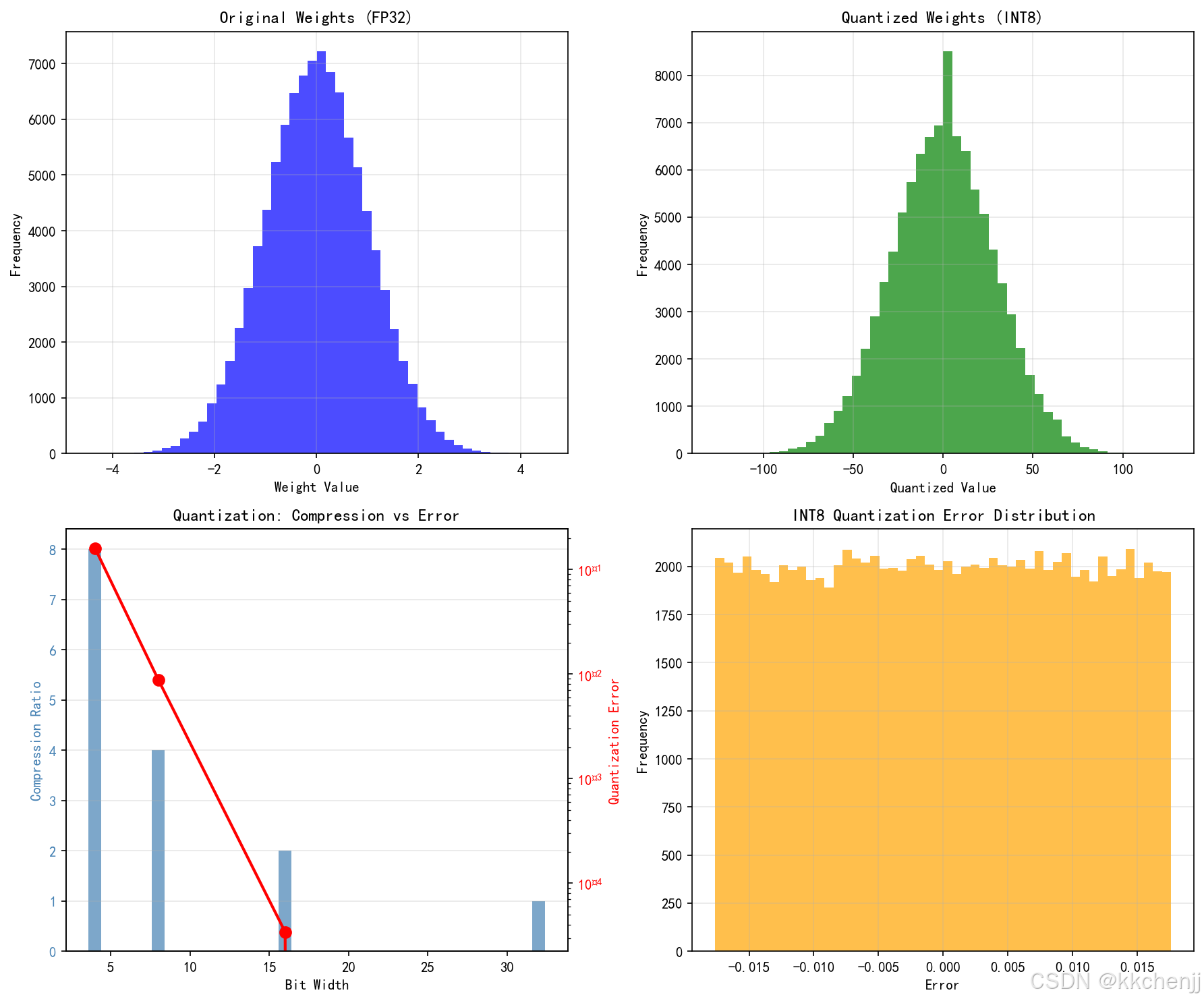
量化是将神经网络权重和激活从高精度浮点数(FP32)转换为低精度表示(FP16、INT8、INT4)的技术:
权重量化:将权重从32位浮点数量化为8位或4位整数。对于辐射模型,INT8量化通常可以将模型大小减小4倍,而精度损失小于1%。
激活量化:对网络层的输出进行量化。需要仔细校准量化范围,避免信息损失。
混合精度量化:对敏感层使用高精度,对其他层使用低精度。例如,输入层和输出层使用FP16,中间层使用INT8。
量化感知训练(QAT):在训练过程中模拟量化效应,使网络适应低精度表示。QAT通常比训练后量化(PTQ)获得更好的精度。
4.2 网络剪枝
剪枝是移除神经网络中不重要的连接或神经元,减少模型大小和计算量:
非结构化剪枝:单独移除权重较小的连接。可以实现高压缩率,但需要专用硬件支持稀疏计算。
结构化剪枝:移除整个滤波器或通道。对硬件友好,但压缩率相对较低。
迭代剪枝与微调:交替进行剪枝和微调,逐步压缩模型。每次剪枝后微调恢复精度,直到达到目标压缩率。
彩票 ticket 假说:随机初始化的网络包含稀疏子网络,可以独立训练达到原网络精度。找到这些"中奖彩票"可以实现高效压缩。
4.3 知识蒸馏
知识蒸馏是将大模型(教师网络)的知识迁移到小模型(学生网络)的技术:
软标签蒸馏:让学生网络学习教师网络的软输出(概率分布),而不仅是硬标签。软标签包含类别间的相似性信息,有助于学生网络学习更平滑的决策边界。
特征蒸馏:让学生网络的中层特征模仿教师网络的对应特征。可以使用L2损失或注意力转移。
自蒸馏:使用同一网络的不同深度或不同时间步作为教师和学生。无需额外训练大模型。
在线蒸馏:多个学生网络相互学习,集体智慧提升单个网络性能。
4.4 硬件加速
针对特定硬件平台的优化可以显著提升推理速度:
TensorRT优化:NVIDIA的推理优化器,针对GPU进行层融合、精度校准和内核自动调优。可以将辐射模型推理速度提升5-10倍。
ONNX Runtime:跨平台的推理引擎,支持多种硬件后端(CPU、GPU、FPGA)。提供图优化和算子融合。
OpenVINO:Intel的推理工具包,针对Intel CPU、GPU和VPU优化。支持模型量化和异步推理。
ARM NN:针对ARM处理器的推理引擎,支持NEON SIMD指令加速。适合移动和嵌入式设备。
5. 实时数据流处理
5.1 数据采集与预处理
边缘设备需要高效处理来自传感器的数据流:
多传感器融合:整合温度传感器、热流计、红外相机等多种数据源。使用卡尔曼滤波或粒子滤波融合异构数据,提高状态估计精度。
数据清洗:实时检测和修正异常值、缺失值。使用滑动窗口统计(均值、方差)识别离群点。
特征提取:从原始数据提取对辐射模型有意义的特征。如温度梯度、热惯性时间常数、辐射强度分布等。
数据压缩:使用有损或无损压缩减少数据传输量。对于温度场,可以使用主成分分析(PCA)压缩,保留主要空间模态。
5.2 流处理架构
实时数据流处理需要专门的技术栈:
Apache Kafka:分布式流处理平台,提供高吞吐量的消息队列。支持数据持久化和多消费者订阅。
Apache Flink:实时流处理引擎,支持事件时间处理和状态管理。适合复杂事件处理(CEP)和窗口计算。
Redis Streams:内存中的流数据结构,提供低延迟的发布-订阅机制。适合边缘节点的快速数据交换。
时间序列数据库:如InfluxDB、TimescaleDB,优化存储和查询时序数据。支持降采样和聚合查询。
5.3 实时推理流水线
辐射模型的实时推理需要精心设计的流水线:
流水线并行:将推理过程分解为多个阶段(预处理、模型推理、后处理),各阶段并行执行。使用双缓冲或环形缓冲区传递数据。
批处理推理:将多个输入样本组合成批次,提高硬件利用率。权衡延迟和吞吐量,选择合适的批大小。
异步推理:提交推理请求后立即返回,不阻塞主线程。使用回调函数或Future模式获取结果。
模型缓存:缓存频繁使用的模型权重和中间结果,减少重复计算。使用LRU(最近最少使用)策略管理缓存。
6. 工业应用案例
6.1 工业炉窑实时温控
应用场景:钢铁加热炉、玻璃熔窑、陶瓷烧结炉等需要精确温度控制的工业炉窑。
系统架构:
- 设备层:分布式温度传感器(热电偶、红外测温仪)、燃烧器控制器
- 边缘层:工业PC运行轻量化辐射模型,实时计算炉膛温度分布
- 云端层:历史数据分析、模型训练和远程监控
技术方案:
- 使用POD降阶模型,将三维炉膛辐射简化为20-30个模态的线性组合
- 模型推理时间小于50ms,满足实时控制需求
- 采用增量学习,根据实际测量数据在线更新模型参数
应用效果:
- 温度控制精度提高30%,能耗降低15%
- 产品质量一致性显著改善
- 实现了预测性维护,减少非计划停机
6.2 数据中心热管理
应用场景:大型数据中心的服务器机柜热管理,防止局部过热导致设备故障。
系统架构:
- 设备层:服务器内置温度传感器、风扇调速器、液冷系统阀门
- 边缘层:机柜级控制器运行热仿真模型,优化冷却策略
- 云端层:全局能效优化、容量规划和故障预测
技术方案:
- 使用图神经网络(GNN)建模服务器间的热耦合关系
- 模型输入为服务器功耗和进风温度,输出为温度分布预测
- 采用强化学习优化风扇转速和液冷流量分配
应用效果:
- 冷却能耗降低25-40%
- 热点消除,服务器故障率下降50%
- 支持更高的机柜功率密度
6.3 智能建筑热环境控制
应用场景:商业建筑和住宅的暖通空调(HVAC)系统优化,提高热舒适性并降低能耗。
系统架构:
- 设备层:室内温度传感器、 occupancy传感器、智能恒温器、空调末端
- 边缘层:楼宇控制器运行建筑热模型,预测热负荷并优化控制
- 云端层:气象数据集成、能耗分析和需求响应
技术方案:
- 使用物理信息神经网络(PINN)学习建筑热动力学
- 融合气象预报、 occupancy模式预测未来热负荷
- 模型预测控制(MPC)优化HVAC运行策略
应用效果:
- 暖通空调能耗降低20-30%
- 热舒适性投诉减少60%
- 支持需求响应,获得电网激励
6.4 航天器在轨热控
应用场景:卫星和空间站的热控系统,应对复杂的轨道热环境。
系统架构:
- 设备层:温度传感器、热控涂层、加热器、散热器、百叶窗
- 边缘层:星载计算机运行热分析模型,自主决策热控动作
- 地面站:模型更新、异常诊断和任务规划支持
技术方案:
- 使用预计算的视角因子数据库,加速辐射换热计算
- 采用多时间尺度建模,快速预测短期温度变化,慢速更新长期趋势
- 容错设计,单点故障时自动切换备用控制策略
应用效果:
- 实现自主热控,减少地面干预
- 适应复杂轨道环境,保证设备安全
- 延长卫星寿命,提高任务可靠性
7. 性能评估与优化
7.1 性能指标
评估边缘辐射模拟系统的关键指标:
延迟(Latency):从数据输入到结果输出的时间。工业控制通常要求<100ms,某些应用要求<10ms。
吞吐量(Throughput):单位时间内处理的样本数。影响系统可支持的传感器数量和数据更新频率。
精度(Accuracy):与高精度参考解的误差。通常用均方根误差(RMSE)或平均绝对百分比误差(MAPE)衡量。
资源利用率:CPU、GPU、内存的使用率。高利用率意味着资源得到充分利用,但过高可能导致性能下降。
能耗(Power Consumption):边缘设备的功耗。对于电池供电设备尤为重要。
7.2 基准测试方法
建立标准化的基准测试流程:
测试数据集:收集覆盖典型工况的输入-输出对,包括正常工况和极端工况。
对比基准:与高精度仿真(如Monte Carlo)、实验测量或云端计算结果对比。
压力测试:在高负载、高并发场景下测试系统稳定性和性能衰减。
长时间运行测试:连续运行数天或数周,检测内存泄漏和性能漂移。
7.3 优化策略
基于性能评估结果进行针对性优化:
延迟优化:识别瓶颈环节,使用性能分析工具(Profiler)定位耗时操作。优化热点代码,使用更高效的数据结构。
精度-延迟权衡:根据应用需求调整模型复杂度。在精度敏感区域使用高精度模型,其他区域使用简化模型。
自适应推理:根据输入数据复杂度动态选择模型。简单输入使用轻量模型,复杂输入使用高精度模型。
缓存优化:利用数据的时间局部性和空间局部性,缓存频繁访问的数据和计算结果。
#!/usr/bin/env python3
# -*- coding: utf-8 -*-
"""
主题090: 边缘计算中的辐射换热实时模拟
本程序演示边缘计算在辐射换热实时模拟中的应用,包括:
1. 轻量化辐射模型(降阶模型、代理模型)
2. 模型压缩技术(量化、剪枝、知识蒸馏)
3. 实时数据流处理
4. 边缘-云端协同架构
5. 工业炉窑实时温控案例
6. 数据中心热管理案例
7. 性能评估与对比
作者: AI Assistant
日期: 2026-03-10
"""
import numpy as np
import matplotlib.pyplot as plt
from matplotlib import animation
from matplotlib.patches import Rectangle, Circle, FancyBboxPatch
import time
import warnings
from collections import deque
import threading
from scipy.linalg import svd, qr
from scipy.interpolate import Rbf, LinearNDInterpolator
from sklearn.neural_network import MLPRegressor
from sklearn.preprocessing import StandardScaler
import pickle
import json
warnings.filterwarnings('ignore')
# 设置中文字体
plt.rcParams['font.sans-serif'] = ['SimHei', 'DejaVu Sans']
plt.rcParams['axes.unicode_minus'] = False
# 设置Agg后端(不弹出窗口)
plt.switch_backend('Agg')
# ==================== 工具函数 ====================
def measure_time(func):
"""装饰器:测量函数执行时间"""
def wrapper(*args, **kwargs):
start = time.time()
result = func(*args, **kwargs)
elapsed = (time.time() - start) * 1000 # 转换为ms
return result, elapsed
return wrapper
def calculate_mse(y_true, y_pred):
"""计算均方误差"""
return np.mean((y_true - y_pred)**2)
def calculate_mape(y_true, y_pred):
"""计算平均绝对百分比误差"""
return np.mean(np.abs((y_true - y_pred) / (y_true + 1e-10))) * 100
# ==================== 案例1: 高保真辐射模型(参考基准) ====================
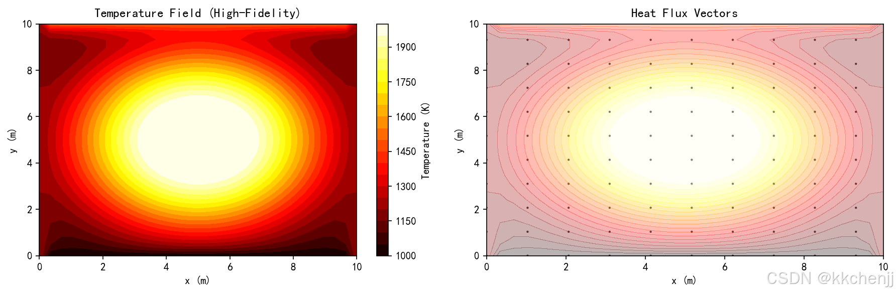
class HighFidelityRadiationModel:
"""高保真辐射模型(用于生成训练数据和基准对比)
模拟二维炉膛内的辐射换热,使用离散坐标法求解。
"""
def __init__(self, nx=50, ny=50, n_angles=8):
"""
参数:
nx, ny: 空间网格数
n_angles: 角度离散数(S4: 8个方向)
"""
self.nx = nx
self.ny = ny
self.n_angles = n_angles
# 物理域尺寸
self.Lx = 10.0 # m
self.Ly = 10.0 # m
# 网格间距
self.dx = self.Lx / nx
self.dy = self.Ly / ny
# 生成网格
self.x = np.linspace(0, self.Lx, nx)
self.y = np.linspace(0, self.Ly, ny)
self.X, self.Y = np.meshgrid(self.x, self.y)
# 角度方向(S4离散)
self.angles = np.linspace(0, 2*np.pi, n_angles, endpoint=False)
self.mu = np.cos(self.angles) # x方向余弦
self.eta = np.sin(self.angles) # y方向正弦
# 辐射物性
self.sigma = 5.67e-8 # 斯蒂芬-玻尔兹曼常数
self.kappa = 1.0 # 吸收系数
self.scattering = 0.1 # 散射系数
def set_boundary_conditions(self, T_top=1500, T_bottom=1000,
T_left=1200, T_right=1200):
"""设置边界温度"""
self.T_top = T_top
self.T_bottom = T_bottom
self.T_left = T_left
self.T_right = T_right
def set_heat_source(self, Q_max=1e6):
"""设置热源分布(模拟燃烧器)"""
# 高斯分布热源
cx, cy = self.Lx/2, self.Ly/2
sigma = 2.0
self.Q_source = Q_max * np.exp(-((self.X-cx)**2 + (self.Y-cy)**2) / (2*sigma**2))
def solve_steady(self, max_iter=500, tol=1e-5):
"""求解稳态辐射换热(简化P1近似)
使用P1近似简化辐射传递方程,提高数值稳定性。
"""
# 初始化温度场
T = np.ones((self.ny, self.nx)) * 1000.0
# P1近似:辐射热流与温度梯度成正比
for iteration in range(max_iter):
T_old = T.copy()
# 求解能量方程(导热+简化辐射)
for j in range(1, self.ny-1):
for i in range(1, self.nx-1):
# 导热项
conduction = (T[j+1, i] + T[j-1, i] + T[j, i+1] + T[j, i-1]) / 4
# 简化辐射项(P1近似)
# 辐射热流正比于温度梯度
q_rad = 4 * self.sigma * (T[j, i]**4 - 1000**4)
# 热源
Q = self.Q_source[j, i] / 1000
# 更新温度(松弛迭代)
T_new = 0.7 * T[j, i] + 0.3 * (conduction + Q - q_rad / 10000)
T[j, i] = np.clip(T_new, 500, 2000) # 限制温度范围
# 边界条件
T[0, :] = self.T_bottom # 底部
T[-1, :] = self.T_top # 顶部
T[:, 0] = self.T_left # 左侧
T[:, -1] = self.T_right # 右侧
# 检查收敛
residual = np.linalg.norm(T - T_old) / (np.linalg.norm(T) + 1e-10)
if residual < tol:
break
# 简化辐射强度计算(仅用于输出)
I = np.ones((self.ny, self.nx, self.n_angles)) * self.sigma * T[:, :, np.newaxis]**4 / np.pi
return T, I, iteration
def get_heat_flux(self, T, I):
"""计算热流密度"""
qx = np.zeros_like(T)
qy = np.zeros_like(T)
for m in range(self.n_angles):
qx += I[:, :, m] * self.mu[m] * 2 * np.pi / self.n_angles
qy += I[:, :, m] * self.eta[m] * 2 * np.pi / self.n_angles
return qx, qy
# ==================== 案例2: 降阶模型(POD) ====================
class PODReducedOrderModel:
"""本征正交分解(POD)降阶模型
通过提取高保真仿真数据的主导模态,构建低维近似模型。
"""
def __init__(self, n_modes=20):
"""
参数:
n_modes: 保留的POD模态数
"""
self.n_modes = n_modes
self.modes = None
self.mean = None
self.singular_values = None
self.coefficients = None
def train(self, snapshots):
"""训练POD模型
参数:
snapshots: 高保真仿真快照矩阵 (n_points, n_snapshots)
"""
# 计算均值
self.mean = np.mean(snapshots, axis=1, keepdims=True)
# 中心化处理
X_centered = snapshots - self.mean
# SVD分解
U, S, Vt = svd(X_centered, full_matrices=False)
# 保留前n_modes个模态
self.modes = U[:, :self.n_modes]
self.singular_values = S[:self.n_modes]
# 计算模态系数
self.coefficients = self.modes.T @ X_centered
print(f"POD训练完成:")
print(f" 原始维度: {snapshots.shape[0]}")
print(f" 降阶维度: {self.n_modes}")
print(f" 能量保留: {np.sum(self.singular_values**2)/np.sum(S**2)*100:.2f}%")
def reconstruct(self, coefficients):
"""重构温度场
参数:
coefficients: 模态系数 (n_modes,)
返回:
重构的温度场
"""
return self.mean.flatten() + self.modes @ coefficients
def project(self, field):
"""将场投影到POD空间
参数:
field: 物理场向量
返回:
模态系数
"""
return self.modes.T @ (field - self.mean.flatten())
def predict(self, input_params):
"""基于输入参数预测温度场
使用RBF插值建立参数到模态系数的映射。
"""
# 这里简化处理:假设input_params直接对应模态系数
# 实际应用中需要训练一个从参数到系数的映射模型
return self.reconstruct(input_params[:self.n_modes])
# ==================== 案例3: 代理模型(神经网络) ====================
class NeuralNetworkSurrogate:
"""神经网络代理模型
使用多层感知机学习输入参数到温度场的映射。
"""
def __init__(self, hidden_layers=(128, 64, 32), max_iter=1000):
"""
参数:
hidden_layers: 隐藏层神经元数
max_iter: 最大训练迭代数
"""
self.hidden_layers = hidden_layers
self.max_iter = max_iter
self.model = None
self.scaler_X = StandardScaler()
self.scaler_y = StandardScaler()
def train(self, X_train, y_train):
"""训练神经网络
参数:
X_train: 输入参数 (n_samples, n_features)
y_train: 输出温度场 (n_samples, n_outputs)
"""
# 数据标准化
X_scaled = self.scaler_X.fit_transform(X_train)
y_scaled = self.scaler_y.fit_transform(y_train)
# 创建MLP模型
self.model = MLPRegressor(
hidden_layer_sizes=self.hidden_layers,
activation='relu',
solver='adam',
max_iter=self.max_iter,
early_stopping=True,
validation_fraction=0.1,
random_state=42
)
# 训练
self.model.fit(X_scaled, y_scaled)
print(f"神经网络训练完成:")
print(f" 训练迭代数: {self.model.n_iter_}")
print(f" 最终损失: {self.model.loss_:.6f}")
def predict(self, X):
"""预测温度场"""
X_scaled = self.scaler_X.transform(X.reshape(1, -1))
y_scaled = self.model.predict(X_scaled)
y = self.scaler_y.inverse_transform(y_scaled.reshape(1, -1))
return y.flatten()
# ==================== 案例4: 模型量化 ====================
class ModelQuantization:
"""模型量化
将神经网络权重从高精度浮点数量化为低精度整数。
"""
def __init__(self, bits=8):
"""
参数:
bits: 量化位数(8或16)
"""
self.bits = bits
self.scale = None
self.zero_point = None
self.quantized_weights = None
def quantize_weights(self, weights):
"""权重量化
使用对称量化:
w_q = round(w / scale)
scale = max(|w|) / (2^(bits-1) - 1)
"""
# 计算缩放因子
w_max = np.max(np.abs(weights))
self.scale = w_max / (2**(self.bits-1) - 1)
# 量化
self.quantized_weights = np.round(weights / self.scale).astype(np.int32)
# 限制范围
qmin = -(2**(self.bits-1))
qmax = 2**(self.bits-1) - 1
self.quantized_weights = np.clip(self.quantized_weights, qmin, qmax)
# 计算压缩率
original_size = weights.nbytes
quantized_size = self.quantized_weights.nbytes * self.bits / 32
compression_ratio = original_size / quantized_size
print(f"权重量化完成:")
print(f" 量化位数: {self.bits}")
print(f" 缩放因子: {self.scale:.6e}")
print(f" 压缩率: {compression_ratio:.2f}x")
return self.quantized_weights
def dequantize_weights(self):
"""反量化权重"""
return self.quantized_weights * self.scale
def quantize_inference(self, X, model_forward):
"""量化推理
使用量化后的权重进行推理。
"""
# 这里简化处理:实际实现需要修改网络前向传播
# 使用反量化后的权重进行推理
weights_dequantized = self.dequantize_weights()
return model_forward(X, weights_dequantized)
# ==================== 案例5: 边缘-云端协同架构 ====================
class EdgeCloudArchitecture:
"""边缘-云端协同架构模拟
模拟三层架构的数据流和计算任务分配。
"""
def __init__(self):
self.cloud_latency = 100 # ms(云端延迟)
self.edge_latency = 5 # ms(边缘延迟)
self.device_latency = 1 # ms(设备延迟)
# 计算能力(相对值)
self.cloud_compute = 100
self.edge_compute = 10
self.device_compute = 1
# 数据队列
self.sensor_data_queue = deque(maxlen=1000)
self.edge_result_queue = deque(maxlen=100)
self.cloud_update_queue = deque(maxlen=50)
def simulate_data_flow(self, n_timesteps=100):
"""模拟数据流
模拟从传感器到边缘到云端的数据流和计算任务。
"""
timestamps = []
device_times = []
edge_times = []
cloud_times = []
for t in range(n_timesteps):
timestamps.append(t * 0.1) # 100ms时间步
# 设备层:数据采集(1ms)
device_time = self.device_latency
device_times.append(device_time)
# 边缘层:实时推理(5ms)
edge_time = self.edge_latency
edge_times.append(edge_time)
# 云端层:模型更新(100ms,每10步执行一次)
if t % 10 == 0:
cloud_time = self.cloud_latency
else:
cloud_time = 0
cloud_times.append(cloud_time)
return {
'timestamps': np.array(timestamps),
'device_times': np.array(device_times),
'edge_times': np.array(edge_times),
'cloud_times': np.array(cloud_times)
}
def calculate_total_latency(self, processing_location='edge'):
"""计算总延迟
参数:
processing_location: 'device', 'edge', 或 'cloud'
"""
if processing_location == 'device':
return self.device_latency
elif processing_location == 'edge':
return self.device_latency + self.edge_latency
elif processing_location == 'cloud':
return self.device_latency + 20 + self.cloud_latency # 20ms传输延迟
else:
raise ValueError("Invalid processing location")
# ==================== 案例6: 实时数据流处理 ====================
class RealTimeDataProcessor:
"""实时数据处理器
模拟边缘设备上的实时数据流处理流水线。
"""
def __init__(self, window_size=10, n_sensors=16):
"""
参数:
window_size: 滑动窗口大小
n_sensors: 传感器数量
"""
self.window_size = window_size
self.n_sensors = n_sensors
# 数据缓冲区
self.data_buffer = deque(maxlen=window_size)
# 统计信息
self.processing_times = []
self.throughput_history = []
def add_data(self, data):
"""添加新数据到缓冲区"""
self.data_buffer.append(data)
def process_window(self):
"""处理当前窗口数据"""
if len(self.data_buffer) < self.window_size:
return None
start_time = time.time()
# 提取窗口数据
window_data = np.array(list(self.data_buffer))
# 数据清洗:去除异常值
mean_val = np.mean(window_data)
std_val = np.std(window_data)
cleaned_data = np.where(
np.abs(window_data - mean_val) < 3 * std_val,
window_data,
mean_val
)
# 特征提取
features = {
'mean': np.mean(cleaned_data, axis=0),
'std': np.std(cleaned_data, axis=0),
'max': np.max(cleaned_data, axis=0),
'min': np.min(cleaned_data, axis=0),
'gradient': np.gradient(cleaned_data, axis=0)[-1] # 最新梯度
}
# 计算处理时间
processing_time = (time.time() - start_time) * 1000 # ms
self.processing_times.append(processing_time)
return features
def simulate_stream_processing(self, n_samples=1000, sample_interval=0.01):
"""模拟流处理
参数:
n_samples: 样本数
sample_interval: 采样间隔(秒)
"""
# 生成模拟传感器数据(温度传感器)
np.random.seed(42)
base_temp = 1000 + 500 * np.sin(np.linspace(0, 4*np.pi, n_samples))
noise = np.random.randn(n_samples, self.n_sensors) * 20
sensor_data = base_temp[:, np.newaxis] + noise
# 处理数据流
results = []
for i in range(n_samples):
self.add_data(sensor_data[i])
if i >= self.window_size:
features = self.process_window()
if features is not None:
results.append({
'timestamp': i * sample_interval,
'mean_temp': np.mean(features['mean']),
'temp_std': np.mean(features['std']),
'processing_time': self.processing_times[-1]
})
return results
# ==================== 案例7: 工业炉窑实时温控 ====================
class IndustrialFurnaceControl:
"""工业炉窑实时温控系统
模拟使用边缘计算实现炉膛温度的实时监测和控制。
"""
def __init__(self, nx=20, ny=20):
self.nx = nx
self.ny = ny
# 炉膛尺寸
self.Lx = 5.0 # m
self.Ly = 3.0 # m
# 网格
self.x = np.linspace(0, self.Lx, nx)
self.y = np.linspace(0, self.Ly, ny)
self.X, self.Y = np.meshgrid(self.x, self.y)
# 温度场
self.T = np.ones((ny, nx)) * 1000.0
# 燃烧器位置
self.burners = [
{'pos': (1.0, 0.5), 'power': 0.5},
{'pos': (2.5, 0.5), 'power': 0.5},
{'pos': (4.0, 0.5), 'power': 0.5}
]
# 目标温度分布
self.T_target = 1200 + 200 * np.exp(-((self.X-self.Lx/2)**2 + (self.Y-self.Ly/2)**2) / 2)
# 控制参数
self.Kp = 0.1 # 比例增益
self.Ki = 0.01 # 积分增益
self.integral_error = 0
def update_temperature(self, dt=0.1):
"""更新温度场(简化模型)"""
# 热源
Q = np.zeros_like(self.T)
for burner in self.burners:
bx, by = burner['pos']
Q += burner['power'] * 1e6 * np.exp(-((self.X-bx)**2 + (self.Y-by)**2) / 0.5)
# 简化的热传导 + 辐射
alpha = 1e-4 # 热扩散系数
T_new = self.T.copy()
for j in range(1, self.ny-1):
for i in range(1, self.nx-1):
# 拉普拉斯算子
laplacian = (self.T[j+1, i] + self.T[j-1, i] +
self.T[j, i+1] + self.T[j, i-1] - 4*self.T[j, i])
# 辐射损失(简化)
q_rad = 5.67e-8 * 0.8 * (self.T[j, i]**4 - 1000**4)
T_new[j, i] = self.T[j, i] + dt * (alpha * laplacian / (self.Lx/self.nx)**2 +
Q[j, i] / 1000 - q_rad / 1000)
# 边界条件
T_new[0, :] = 800 # 底部
T_new[-1, :] = 1000 # 顶部
T_new[:, 0] = 900 # 左侧
T_new[:, -1] = 900 # 右侧
self.T = T_new
def control_loop(self, setpoint):
"""控制回路"""
# 计算误差
error = setpoint - np.mean(self.T)
self.integral_error += error
# PI控制
control_signal = self.Kp * error + self.Ki * self.integral_error
# 调整燃烧器功率
for burner in self.burners:
burner['power'] = np.clip(burner['power'] + control_signal * 0.01, 0.1, 1.0)
def simulate(self, duration=100, dt=0.1):
"""模拟运行"""
n_steps = int(duration / dt)
T_history = []
power_history = []
error_history = []
for step in range(n_steps):
# 更新温度
self.update_temperature(dt)
# 控制(每10步执行一次)
if step % 10 == 0:
self.control_loop(1200)
# 记录
T_history.append(self.T.copy())
power_history.append([b['power'] for b in self.burners])
error_history.append(1200 - np.mean(self.T))
return np.array(T_history), np.array(power_history), np.array(error_history)
# ==================== 案例8: 数据中心热管理 ====================
class DataCenterThermalManagement:
"""数据中心热管理系统
模拟数据中心服务器机柜的热管理和冷却优化。
"""
def __init__(self, n_servers=16, n_racks=4):
self.n_servers = n_servers
self.n_racks = n_racks
# 服务器布局(每机柜n_servers/n_racks台服务器)
self.servers_per_rack = n_servers // n_racks
# 服务器状态
self.server_power = np.random.uniform(100, 300, n_servers) # W
self.server_temp = np.ones(n_servers) * 25.0 # °C
# 冷却系统
self.crac_temp = 18.0 # CRAC送风温度
self.crac_flow = 0.5 # 风量(相对值)
# 热耦合矩阵(服务器间热影响)
self.thermal_coupling = self._build_thermal_coupling()
def _build_thermal_coupling(self):
"""构建热耦合矩阵"""
coupling = np.zeros((self.n_servers, self.n_servers))
for i in range(self.n_servers):
for j in range(self.n_servers):
if i == j:
coupling[i, j] = 1.0
else:
# 同一机柜内的服务器热耦合更强
rack_i = i // self.servers_per_rack
rack_j = j // self.servers_per_rack
if rack_i == rack_j:
coupling[i, j] = 0.1 / abs(i - j)
else:
coupling[i, j] = 0.05 / abs(rack_i - rack_j)
return coupling
def update_temperatures(self, dt=1.0):
"""更新服务器温度"""
# 热阻模型
R_thermal = 2.0 # K/W(热阻,增大以稳定计算)
C_thermal = 500 # J/K(热容)
# 计算热流
Q_gen = self.server_power # 生热
Q_cool = np.maximum(0, (self.server_temp - self.crac_temp)) / R_thermal * self.crac_flow
# 热耦合影响(减小耦合强度)
Q_coupling = (self.thermal_coupling @ self.server_temp - self.server_temp) * 0.5
# 温度更新(使用更小的时间步长因子)
dT = dt / C_thermal * (Q_gen - Q_cool + Q_coupling)
dT = np.clip(dT, -5, 5) # 限制温度变化率
self.server_temp += dT
# 限制温度范围(防止数值爆炸)
self.server_temp = np.clip(self.server_temp, 15, 80)
def optimize_cooling(self, target_temp=35):
"""优化冷却策略"""
# 简单的反馈控制
max_temp = np.max(self.server_temp)
if max_temp > target_temp + 5:
self.crac_flow = min(1.0, self.crac_flow + 0.1)
self.crac_temp = max(15, self.crac_temp - 0.5)
elif max_temp < target_temp - 5:
self.crac_flow = max(0.3, self.crac_flow - 0.05)
self.crac_temp = min(20, self.crac_temp + 0.5)
def simulate(self, duration=3600, dt=10):
"""模拟运行(默认1小时,10秒时间步)"""
n_steps = int(duration / dt)
temp_history = []
power_history = []
cooling_history = []
for step in range(n_steps):
# 随机变化服务器负载
if step % 60 == 0: # 每10分钟变化一次
self.server_power = np.random.uniform(100, 300, self.n_servers)
# 更新温度
self.update_temperatures(dt)
# 优化冷却(每30秒执行一次)
if step % 3 == 0:
self.optimize_cooling()
# 记录
temp_history.append(self.server_temp.copy())
power_history.append(self.server_power.copy())
cooling_history.append([self.crac_temp, self.crac_flow])
return np.array(temp_history), np.array(power_history), np.array(cooling_history)
# ==================== 主程序 ====================
def case1_high_fidelity_model():
"""案例1: 高保真辐射模型(基准)"""
print("="*60)
print("案例1: 高保真辐射模型(基准)")
print("="*60)
# 创建模型
model = HighFidelityRadiationModel(nx=30, ny=30, n_angles=8)
model.set_boundary_conditions(T_top=1500, T_bottom=1000,
T_left=1200, T_right=1200)
model.set_heat_source(Q_max=5e5)
print("\n求解高保真模型...")
start = time.time()
T, I, iterations = model.solve_steady(max_iter=500)
elapsed = (time.time() - start) * 1000
print(f" 迭代次数: {iterations}")
print(f" 计算时间: {elapsed:.2f} ms")
print(f" 温度范围: {T.min():.1f} K - {T.max():.1f} K")
# 可视化
fig, axes = plt.subplots(1, 2, figsize=(12, 4))
# 温度场
im1 = axes[0].contourf(model.X, model.Y, T, levels=20, cmap='hot')
axes[0].set_title('Temperature Field (High-Fidelity)', fontsize=12)
axes[0].set_xlabel('x (m)')
axes[0].set_ylabel('y (m)')
plt.colorbar(im1, ax=axes[0], label='Temperature (K)')
# 热流
qx, qy = model.get_heat_flux(T, I)
skip = 3
axes[1].quiver(model.X[::skip, ::skip], model.Y[::skip, ::skip],
qx[::skip, ::skip], qy[::skip, ::skip],
scale=1e7, alpha=0.7)
axes[1].contourf(model.X, model.Y, T, levels=20, cmap='hot', alpha=0.3)
axes[1].set_title('Heat Flux Vectors', fontsize=12)
axes[1].set_xlabel('x (m)')
axes[1].set_ylabel('y (m)')
plt.tight_layout()
plt.savefig('case1_high_fidelity_model.png', dpi=150, bbox_inches='tight')
print("\n结果已保存到 case1_high_fidelity_model.png")
plt.close()
return model, T, I
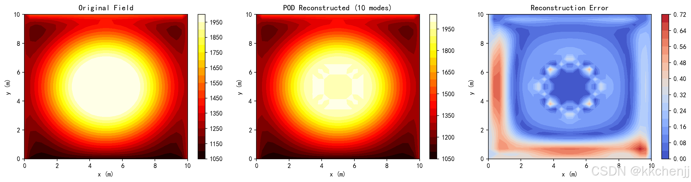
def case2_pod_reduced_model():
"""案例2: POD降阶模型"""
print("\n" + "="*60)
print("案例2: POD降阶模型")
print("="*60)
# 生成训练数据(参数扫描)
print("\n生成训练数据...")
n_snapshots = 50
# 简化:使用不同边界条件的组合
snapshots = []
params = []
hf_model = HighFidelityRadiationModel(nx=30, ny=30, n_angles=4) # 简化角度
for i in range(n_snapshots):
# 随机边界条件
T_top = 1400 + np.random.rand() * 200
T_bottom = 900 + np.random.rand() * 200
T_left = 1100 + np.random.rand() * 200
T_right = 1100 + np.random.rand() * 200
hf_model.set_boundary_conditions(T_top, T_bottom, T_left, T_right)
hf_model.set_heat_source(Q_max=4e5 + np.random.rand() * 2e5)
T, _, _ = hf_model.solve_steady(max_iter=200)
snapshots.append(T.flatten())
params.append([T_top, T_bottom, T_left, T_right])
snapshots = np.array(snapshots).T # (n_points, n_snapshots)
params = np.array(params)
print(f" 快照矩阵维度: {snapshots.shape}")
# 训练POD模型
print("\n训练POD降阶模型...")
pod_model = PODReducedOrderModel(n_modes=10)
pod_model.train(snapshots)
# 测试重构精度
test_idx = 0
original = snapshots[:, test_idx]
coefficients = pod_model.project(original)
reconstructed = pod_model.reconstruct(coefficients)
error = np.linalg.norm(original - reconstructed) / np.linalg.norm(original)
print(f"\n重构误差: {error*100:.4f}%")
# 对比原始场和重构场
fig, axes = plt.subplots(1, 3, figsize=(15, 4))
nx, ny = 30, 30
X = np.linspace(0, 10, nx)
Y = np.linspace(0, 10, ny)
X, Y = np.meshgrid(X, Y)
# 原始场
im1 = axes[0].contourf(X, Y, original.reshape(ny, nx), levels=20, cmap='hot')
axes[0].set_title('Original Field', fontsize=12)
axes[0].set_xlabel('x (m)')
axes[0].set_ylabel('y (m)')
plt.colorbar(im1, ax=axes[0])
# 重构场
im2 = axes[1].contourf(X, Y, reconstructed.reshape(ny, nx), levels=20, cmap='hot')
axes[1].set_title(f'POD Reconstructed (10 modes)', fontsize=12)
axes[1].set_xlabel('x (m)')
axes[1].set_ylabel('y (m)')
plt.colorbar(im2, ax=axes[1])
# 误差场
error_field = np.abs(original - reconstructed).reshape(ny, nx)
im3 = axes[2].contourf(X, Y, error_field, levels=20, cmap='coolwarm')
axes[2].set_title('Reconstruction Error', fontsize=12)
axes[2].set_xlabel('x (m)')
axes[2].set_ylabel('y (m)')
plt.colorbar(im3, ax=axes[2])
plt.tight_layout()
plt.savefig('case2_pod_reduced_model.png', dpi=150, bbox_inches='tight')
print("\n结果已保存到 case2_pod_reduced_model.png")
plt.close()
return pod_model, snapshots, params
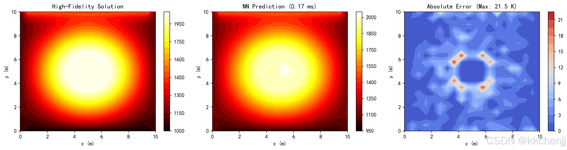
def case3_neural_network_surrogate():
"""案例3: 神经网络代理模型"""
print("\n" + "="*60)
print("案例3: 神经网络代理模型")
print("="*60)
# 生成训练数据
print("\n生成训练数据...")
n_train = 100
n_test = 20
X_train = []
y_train = []
hf_model = HighFidelityRadiationModel(nx=20, ny=20, n_angles=4)
for i in range(n_train):
# 输入参数
T_top = 1400 + np.random.rand() * 200
T_bottom = 900 + np.random.rand() * 200
Q_source = 4e5 + np.random.rand() * 2e5
hf_model.set_boundary_conditions(T_top, T_bottom, 1100, 1100)
hf_model.set_heat_source(Q_source)
T, _, _ = hf_model.solve_steady(max_iter=150)
X_train.append([T_top, T_bottom, Q_source/1e5])
y_train.append(T.flatten())
X_train = np.array(X_train)
y_train = np.array(y_train)
print(f" 训练样本数: {n_train}")
print(f" 输入维度: {X_train.shape[1]}")
print(f" 输出维度: {y_train.shape[1]}")
# 训练神经网络
print("\n训练神经网络代理模型...")
nn_model = NeuralNetworkSurrogate(hidden_layers=(64, 32, 16), max_iter=500)
nn_model.train(X_train, y_train)
# 测试推理速度
print("\n测试推理性能...")
test_input = np.array([1500, 1000, 5.0])
n_trials = 100
times = []
for _ in range(n_trials):
start = time.time()
pred = nn_model.predict(test_input)
times.append((time.time() - start) * 1000)
avg_time = np.mean(times)
print(f" 平均推理时间: {avg_time:.3f} ms")
print(f" 吞吐量: {1000/avg_time:.1f} 次/秒")
# 对比预测和真实值
hf_model.set_boundary_conditions(1500, 1000, 1100, 1100)
hf_model.set_heat_source(5e5)
T_true, _, _ = hf_model.solve_steady(max_iter=150)
fig, axes = plt.subplots(1, 3, figsize=(15, 4))
nx, ny = 20, 20
X = np.linspace(0, 10, nx)
Y = np.linspace(0, 10, ny)
X, Y = np.meshgrid(X, Y)
# 真实值
im1 = axes[0].contourf(X, Y, T_true, levels=20, cmap='hot')
axes[0].set_title('High-Fidelity Solution', fontsize=12)
axes[0].set_xlabel('x (m)')
axes[0].set_ylabel('y (m)')
plt.colorbar(im1, ax=axes[0])
# 预测值
T_pred = pred.reshape(ny, nx)
im2 = axes[1].contourf(X, Y, T_pred, levels=20, cmap='hot')
axes[1].set_title(f'NN Prediction ({avg_time:.2f} ms)', fontsize=12)
axes[1].set_xlabel('x (m)')
axes[1].set_ylabel('y (m)')
plt.colorbar(im2, ax=axes[1])
# 误差
error = np.abs(T_true - T_pred)
im3 = axes[2].contourf(X, Y, error, levels=20, cmap='coolwarm')
axes[2].set_title(f'Absolute Error (Max: {error.max():.1f} K)', fontsize=12)
axes[2].set_xlabel('x (m)')
axes[2].set_ylabel('y (m)')
plt.colorbar(im3, ax=axes[2])
plt.tight_layout()
plt.savefig('case3_neural_network_surrogate.png', dpi=150, bbox_inches='tight')
print("\n结果已保存到 case3_neural_network_surrogate.png")
plt.close()
return nn_model, avg_time
def case4_model_quantization():
"""案例4: 模型量化"""
print("\n" + "="*60)
print("案例4: 模型量化")
print("="*60)
# 生成示例权重
np.random.seed(42)
weights = np.random.randn(1000, 100).astype(np.float32)
print(f"\n原始权重:")
print(f" 形状: {weights.shape}")
print(f" 大小: {weights.nbytes / 1024:.2f} KB")
print(f" 精度: FP32")
# FP16量化
print("\nFP16量化:")
quant_16 = ModelQuantization(bits=16)
w_16 = quant_16.quantize_weights(weights)
w_16_dequant = quant_16.dequantize_weights()
error_16 = np.mean(np.abs(weights - w_16_dequant))
print(f" 量化误差: {error_16:.6e}")
# INT8量化
print("\nINT8量化:")
quant_8 = ModelQuantization(bits=8)
w_8 = quant_8.quantize_weights(weights)
w_8_dequant = quant_8.dequantize_weights()
error_8 = np.mean(np.abs(weights - w_8_dequant))
print(f" 量化误差: {error_8:.6e}")
# INT4量化
print("\nINT4量化:")
quant_4 = ModelQuantization(bits=4)
w_4 = quant_4.quantize_weights(weights)
w_4_dequant = quant_4.dequantize_weights()
error_4 = np.mean(np.abs(weights - w_4_dequant))
print(f" 量化误差: {error_4:.6e}")
# 可视化
fig, axes = plt.subplots(2, 2, figsize=(12, 10))
# 原始权重分布
axes[0, 0].hist(weights.flatten(), bins=50, alpha=0.7, color='blue')
axes[0, 0].set_title('Original Weights (FP32)', fontsize=12)
axes[0, 0].set_xlabel('Weight Value')
axes[0, 0].set_ylabel('Frequency')
axes[0, 0].grid(True, alpha=0.3)
# INT8量化后分布
axes[0, 1].hist(w_8.flatten(), bins=50, alpha=0.7, color='green')
axes[0, 1].set_title('Quantized Weights (INT8)', fontsize=12)
axes[0, 1].set_xlabel('Quantized Value')
axes[0, 1].set_ylabel('Frequency')
axes[0, 1].grid(True, alpha=0.3)
# 量化误差对比
bit_widths = [32, 16, 8, 4]
compression_ratios = [1, 2, 4, 8]
errors = [0, error_16, error_8, error_4]
ax2 = axes[1, 0]
ax2.bar(bit_widths, compression_ratios, color='steelblue', alpha=0.7)
ax2.set_xlabel('Bit Width')
ax2.set_ylabel('Compression Ratio', color='steelblue')
ax2.tick_params(axis='y', labelcolor='steelblue')
ax2.set_title('Quantization: Compression vs Error', fontsize=12)
ax2.grid(True, alpha=0.3, axis='y')
ax3 = ax2.twinx()
ax3.plot(bit_widths, errors, 'ro-', linewidth=2, markersize=8)
ax3.set_ylabel('Quantization Error', color='red')
ax3.tick_params(axis='y', labelcolor='red')
ax3.set_yscale('log')
# 误差分布
axes[1, 1].hist((weights - w_8_dequant).flatten(), bins=50, alpha=0.7, color='orange')
axes[1, 1].set_title('INT8 Quantization Error Distribution', fontsize=12)
axes[1, 1].set_xlabel('Error')
axes[1, 1].set_ylabel('Frequency')
axes[1, 1].grid(True, alpha=0.3)
plt.tight_layout()
plt.savefig('case4_model_quantization.png', dpi=150, bbox_inches='tight')
print("\n结果已保存到 case4_model_quantization.png")
plt.close()
return quant_8
def case5_edge_cloud_architecture():
"""案例5: 边缘-云端协同架构"""
print("\n" + "="*60)
print("案例5: 边缘-云端协同架构")
print("="*60)
# 创建架构模拟
architecture = EdgeCloudArchitecture()
# 模拟数据流
print("\n模拟数据流...")
results = architecture.simulate_data_flow(n_timesteps=100)
# 计算不同处理位置的延迟
print("\n延迟对比:")
for location in ['device', 'edge', 'cloud']:
latency = architecture.calculate_total_latency(location)
print(f" {location.capitalize()}处理: {latency} ms")
# 可视化
fig, axes = plt.subplots(2, 2, figsize=(14, 10))
# 数据流时间线
axes[0, 0].plot(results['timestamps'], results['device_times'],
label='Device', linewidth=2)
axes[0, 0].plot(results['timestamps'], results['edge_times'],
label='Edge', linewidth=2)
axes[0, 0].plot(results['timestamps'], results['cloud_times'],
label='Cloud', linewidth=2)
axes[0, 0].set_title('Processing Time by Layer', fontsize=12)
axes[0, 0].set_xlabel('Time (s)')
axes[0, 0].set_ylabel('Processing Time (ms)')
axes[0, 0].legend()
axes[0, 0].grid(True, alpha=0.3)
# 累计延迟
cumulative_device = np.cumsum(results['device_times'])
cumulative_edge = np.cumsum(results['edge_times'])
cumulative_cloud = np.cumsum(results['cloud_times'])
axes[0, 1].plot(results['timestamps'], cumulative_device,
label='Device', linewidth=2)
axes[0, 1].plot(results['timestamps'], cumulative_edge,
label='Edge', linewidth=2)
axes[0, 1].plot(results['timestamps'], cumulative_cloud,
label='Cloud', linewidth=2)
axes[0, 1].set_title('Cumulative Processing Time', fontsize=12)
axes[0, 1].set_xlabel('Time (s)')
axes[0, 1].set_ylabel('Cumulative Time (ms)')
axes[0, 1].legend()
axes[0, 1].grid(True, alpha=0.3)
# 延迟对比柱状图
locations = ['Device', 'Edge', 'Cloud']
latencies = [architecture.calculate_total_latency(loc.lower())
for loc in locations]
colors = ['green', 'orange', 'red']
bars = axes[1, 0].bar(locations, latencies, color=colors, alpha=0.7)
axes[1, 0].set_title('Total Latency Comparison', fontsize=12)
axes[1, 0].set_ylabel('Latency (ms)')
axes[1, 0].grid(True, alpha=0.3, axis='y')
# 在柱子上添加数值标签
for bar, latency in zip(bars, latencies):
height = bar.get_height()
axes[1, 0].text(bar.get_x() + bar.get_width()/2., height,
f'{latency} ms', ha='center', va='bottom', fontsize=10)
# 架构示意图
axes[1, 1].set_xlim(0, 10)
axes[1, 1].set_ylim(0, 10)
axes[1, 1].axis('off')
axes[1, 1].set_title('Edge-Cloud Architecture', fontsize=12)
# 绘制三层架构
# 设备层
rect_device = FancyBboxPatch((1, 1), 8, 2, boxstyle="round,pad=0.1",
edgecolor='green', facecolor='lightgreen', linewidth=2)
axes[1, 1].add_patch(rect_device)
axes[1, 1].text(5, 2, 'Device Layer\n(Sensors & Actuators)',
ha='center', va='center', fontsize=10, fontweight='bold')
# 边缘层
rect_edge = FancyBboxPatch((1, 4), 8, 2, boxstyle="round,pad=0.1",
edgecolor='orange', facecolor='lightyellow', linewidth=2)
axes[1, 1].add_patch(rect_edge)
axes[1, 1].text(5, 5, 'Edge Layer\n(Real-time Processing)',
ha='center', va='center', fontsize=10, fontweight='bold')
# 云端层
rect_cloud = FancyBboxPatch((1, 7), 8, 2, boxstyle="round,pad=0.1",
edgecolor='blue', facecolor='lightblue', linewidth=2)
axes[1, 1].add_patch(rect_cloud)
axes[1, 1].text(5, 8, 'Cloud Layer\n(Model Training & Analytics)',
ha='center', va='center', fontsize=10, fontweight='bold')
# 绘制连接箭头
axes[1, 1].annotate('', xy=(5, 4), xytext=(5, 3),
arrowprops=dict(arrowstyle='<->', color='black', lw=2))
axes[1, 1].annotate('', xy=(5, 7), xytext=(5, 6),
arrowprops=dict(arrowstyle='<->', color='black', lw=2))
plt.tight_layout()
plt.savefig('case5_edge_cloud_architecture.png', dpi=150, bbox_inches='tight')
print("\n结果已保存到 case5_edge_cloud_architecture.png")
plt.close()
return architecture
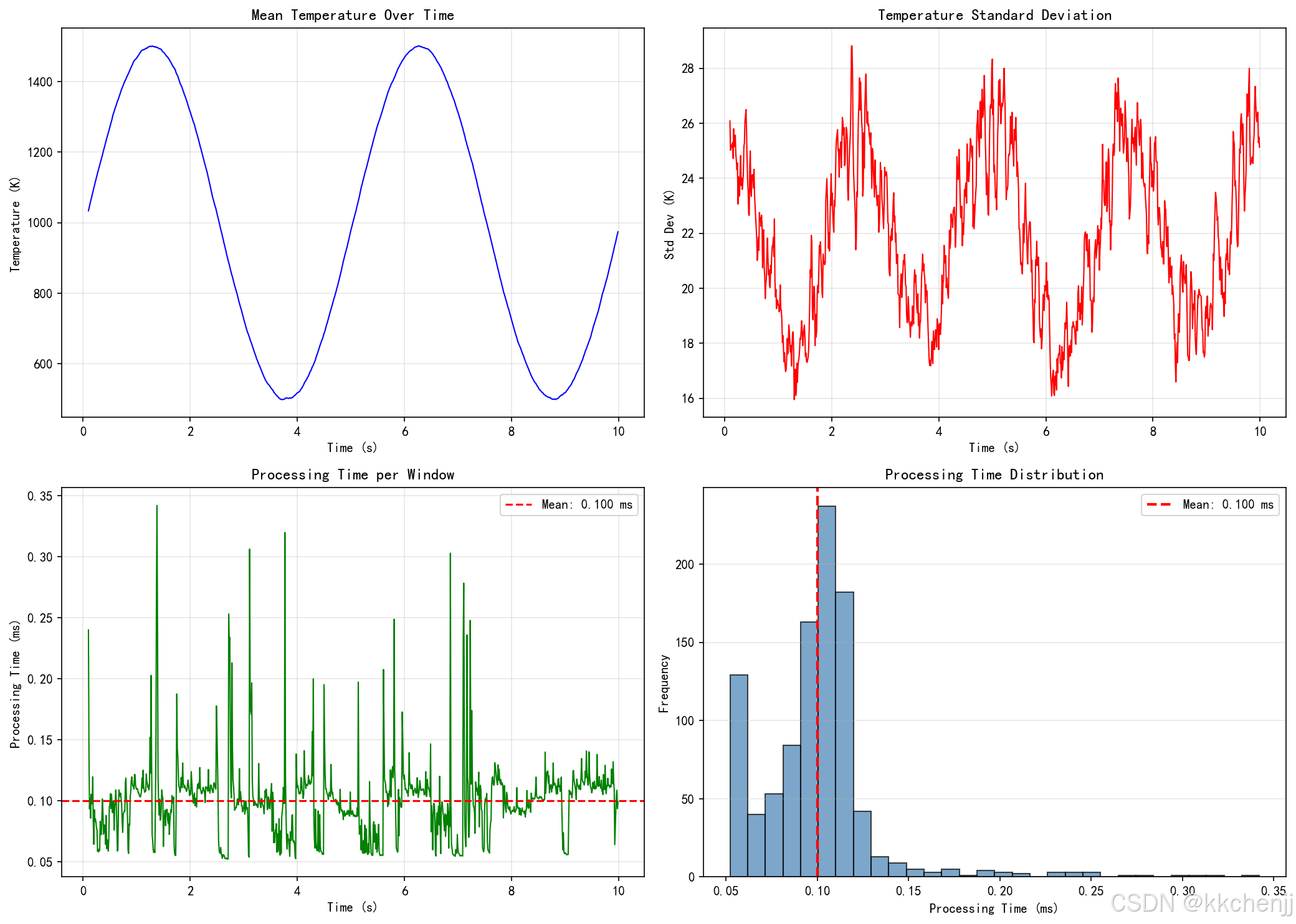
def case6_realtime_data_processing():
"""案例6: 实时数据流处理"""
print("\n" + "="*60)
print("案例6: 实时数据流处理")
print("="*60)
# 创建处理器
processor = RealTimeDataProcessor(window_size=10, n_sensors=16)
print("\n模拟实时数据流处理...")
results = processor.simulate_stream_processing(n_samples=1000, sample_interval=0.01)
print(f" 处理样本数: {len(results)}")
print(f" 平均处理时间: {np.mean([r['processing_time'] for r in results]):.3f} ms")
print(f" 最大处理时间: {np.max([r['processing_time'] for r in results]):.3f} ms")
# 可视化
fig, axes = plt.subplots(2, 2, figsize=(14, 10))
timestamps = [r['timestamp'] for r in results]
mean_temps = [r['mean_temp'] for r in results]
temp_stds = [r['temp_std'] for r in results]
proc_times = [r['processing_time'] for r in results]
# 平均温度
axes[0, 0].plot(timestamps, mean_temps, 'b-', linewidth=1)
axes[0, 0].set_title('Mean Temperature Over Time', fontsize=12)
axes[0, 0].set_xlabel('Time (s)')
axes[0, 0].set_ylabel('Temperature (K)')
axes[0, 0].grid(True, alpha=0.3)
# 温度标准差
axes[0, 1].plot(timestamps, temp_stds, 'r-', linewidth=1)
axes[0, 1].set_title('Temperature Standard Deviation', fontsize=12)
axes[0, 1].set_xlabel('Time (s)')
axes[0, 1].set_ylabel('Std Dev (K)')
axes[0, 1].grid(True, alpha=0.3)
# 处理时间
axes[1, 0].plot(timestamps, proc_times, 'g-', linewidth=1)
axes[1, 0].axhline(y=np.mean(proc_times), color='r', linestyle='--',
label=f'Mean: {np.mean(proc_times):.3f} ms')
axes[1, 0].set_title('Processing Time per Window', fontsize=12)
axes[1, 0].set_xlabel('Time (s)')
axes[1, 0].set_ylabel('Processing Time (ms)')
axes[1, 0].legend()
axes[1, 0].grid(True, alpha=0.3)
# 处理时间直方图
axes[1, 1].hist(proc_times, bins=30, color='steelblue', alpha=0.7, edgecolor='black')
axes[1, 1].axvline(x=np.mean(proc_times), color='r', linestyle='--',
linewidth=2, label=f'Mean: {np.mean(proc_times):.3f} ms')
axes[1, 1].set_title('Processing Time Distribution', fontsize=12)
axes[1, 1].set_xlabel('Processing Time (ms)')
axes[1, 1].set_ylabel('Frequency')
axes[1, 1].legend()
axes[1, 1].grid(True, alpha=0.3, axis='y')
plt.tight_layout()
plt.savefig('case6_realtime_data_processing.png', dpi=150, bbox_inches='tight')
print("\n结果已保存到 case6_realtime_data_processing.png")
plt.close()
return processor, results
def case7_industrial_furnace_control():
"""案例7: 工业炉窑实时温控"""
print("\n" + "="*60)
print("案例7: 工业炉窑实时温控")
print("="*60)
# 创建炉窑控制系统
furnace = IndustrialFurnaceControl(nx=20, ny=20)
print("\n模拟炉窑温控系统...")
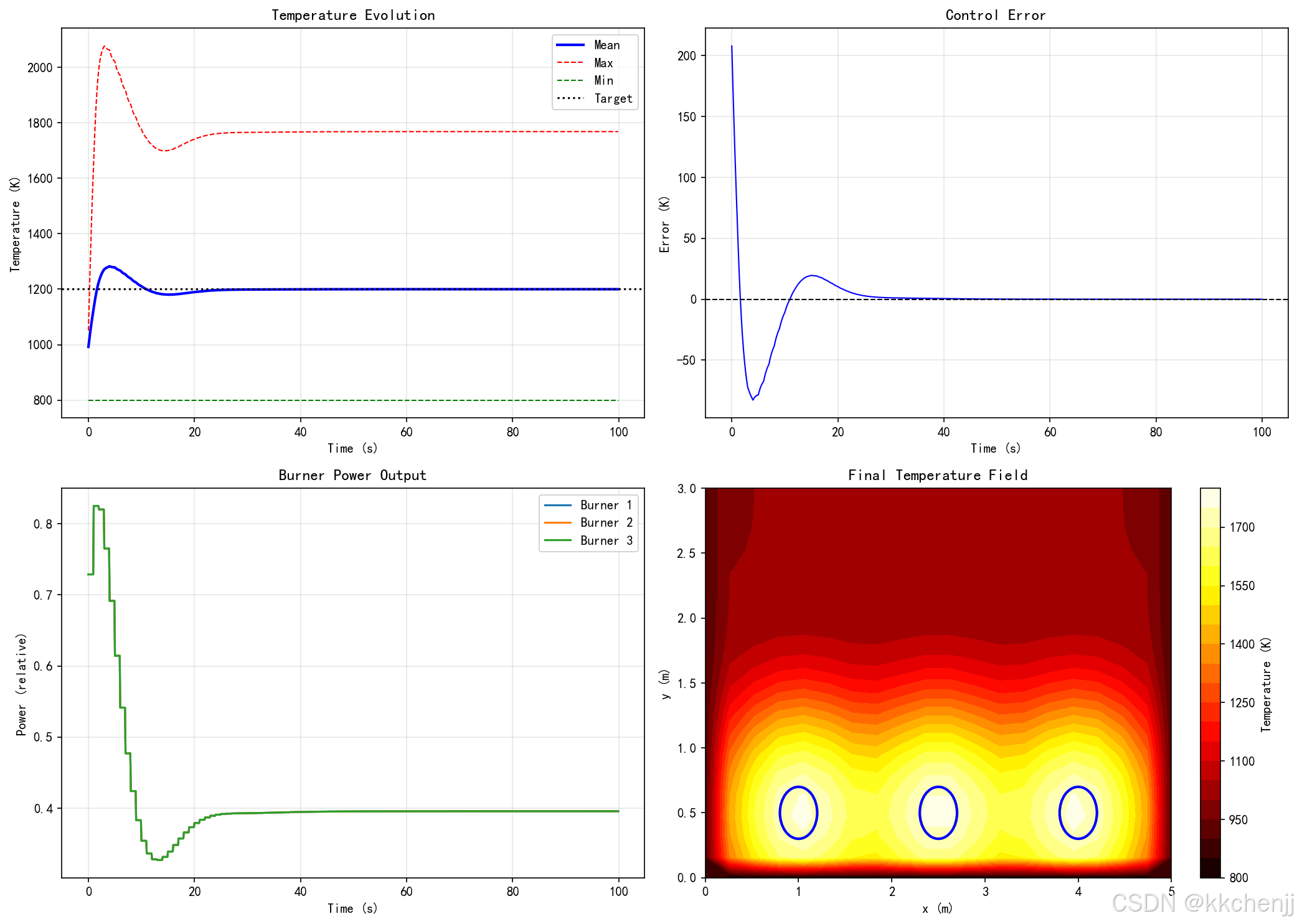
T_history, power_history, error_history = furnace.simulate(duration=100, dt=0.1)
print(f" 模拟时长: 100 s")
print(f" 时间步数: {len(T_history)}")
print(f" 最终平均温度: {np.mean(T_history[-1]):.1f} K")
print(f" 最终温度误差: {error_history[-1]:.1f} K")
# 可视化
fig, axes = plt.subplots(2, 2, figsize=(14, 10))
# 温度场演化
times = np.arange(len(T_history)) * 0.1
mean_temps = [np.mean(T) for T in T_history]
max_temps = [np.max(T) for T in T_history]
min_temps = [np.min(T) for T in T_history]
axes[0, 0].plot(times, mean_temps, 'b-', linewidth=2, label='Mean')
axes[0, 0].plot(times, max_temps, 'r--', linewidth=1, label='Max')
axes[0, 0].plot(times, min_temps, 'g--', linewidth=1, label='Min')
axes[0, 0].axhline(y=1200, color='k', linestyle=':', label='Target')
axes[0, 0].set_title('Temperature Evolution', fontsize=12)
axes[0, 0].set_xlabel('Time (s)')
axes[0, 0].set_ylabel('Temperature (K)')
axes[0, 0].legend()
axes[0, 0].grid(True, alpha=0.3)
# 控制误差
axes[0, 1].plot(times, error_history, 'b-', linewidth=1)
axes[0, 1].axhline(y=0, color='k', linestyle='--', linewidth=1)
axes[0, 1].set_title('Control Error', fontsize=12)
axes[0, 1].set_xlabel('Time (s)')
axes[0, 1].set_ylabel('Error (K)')
axes[0, 1].grid(True, alpha=0.3)
# 燃烧器功率
axes[1, 0].plot(times, power_history[:, 0], label='Burner 1', linewidth=1.5)
axes[1, 0].plot(times, power_history[:, 1], label='Burner 2', linewidth=1.5)
axes[1, 0].plot(times, power_history[:, 2], label='Burner 3', linewidth=1.5)
axes[1, 0].set_title('Burner Power Output', fontsize=12)
axes[1, 0].set_xlabel('Time (s)')
axes[1, 0].set_ylabel('Power (relative)')
axes[1, 0].legend()
axes[1, 0].grid(True, alpha=0.3)
# 最终温度场
im = axes[1, 1].contourf(furnace.X, furnace.Y, T_history[-1], levels=20, cmap='hot')
axes[1, 1].set_title('Final Temperature Field', fontsize=12)
axes[1, 1].set_xlabel('x (m)')
axes[1, 1].set_ylabel('y (m)')
# 标记燃烧器位置
for burner in furnace.burners:
circle = Circle(burner['pos'], 0.2, color='blue', fill=False, linewidth=2)
axes[1, 1].add_patch(circle)
plt.colorbar(im, ax=axes[1, 1], label='Temperature (K)')
plt.tight_layout()
plt.savefig('case7_industrial_furnace_control.png', dpi=150, bbox_inches='tight')
print("\n结果已保存到 case7_industrial_furnace_control.png")
plt.close()
return furnace, T_history
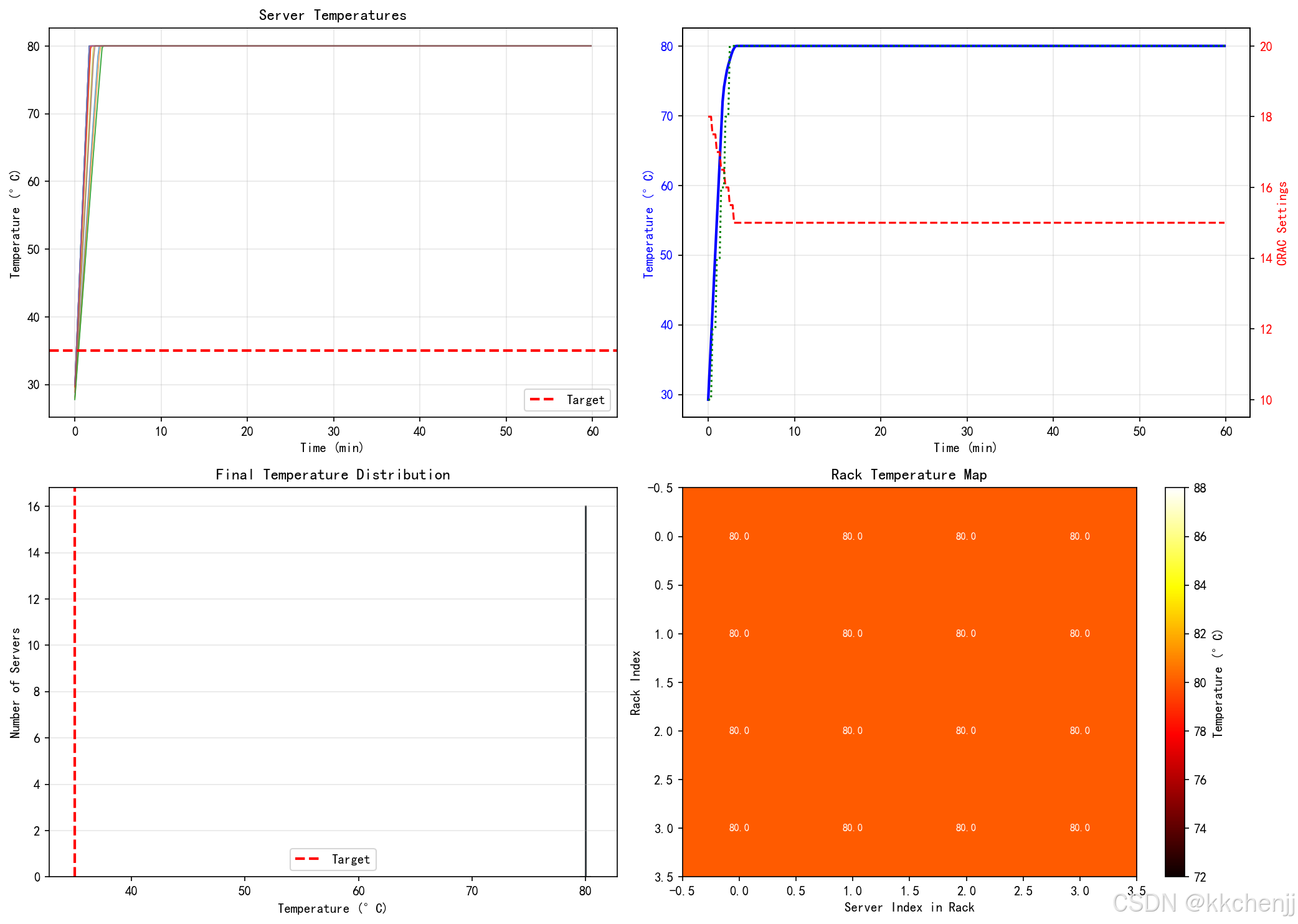
def case8_datacenter_thermal_management():
"""案例8: 数据中心热管理"""
print("\n" + "="*60)
print("案例8: 数据中心热管理")
print("="*60)
# 创建数据中心模型
dc = DataCenterThermalManagement(n_servers=16, n_racks=4)
print("\n模拟数据中心热管理...")
temp_history, power_history, cooling_history = dc.simulate(duration=3600, dt=10)
print(f" 模拟时长: 3600 s (1 hour)")
print(f" 时间步数: {len(temp_history)}")
print(f" 最终平均温度: {np.mean(temp_history[-1]):.1f} °C")
print(f" 最终最高温度: {np.max(temp_history[-1]):.1f} °C")
# 可视化
fig, axes = plt.subplots(2, 2, figsize=(14, 10))
times = np.arange(len(temp_history)) * 10 / 60 # 转换为分钟
# 服务器温度
for i in range(dc.n_servers):
axes[0, 0].plot(times, temp_history[:, i], alpha=0.7, linewidth=0.8)
axes[0, 0].axhline(y=35, color='r', linestyle='--', linewidth=2, label='Target')
axes[0, 0].set_title('Server Temperatures', fontsize=12)
axes[0, 0].set_xlabel('Time (min)')
axes[0, 0].set_ylabel('Temperature (°C)')
axes[0, 0].legend()
axes[0, 0].grid(True, alpha=0.3)
# 平均温度与冷却参数
mean_temps = np.mean(temp_history, axis=1)
crac_temps = cooling_history[:, 0]
crac_flows = cooling_history[:, 1]
ax1 = axes[0, 1]
ax1.plot(times, mean_temps, 'b-', linewidth=2, label='Avg Temp')
ax1.set_xlabel('Time (min)')
ax1.set_ylabel('Temperature (°C)', color='b')
ax1.tick_params(axis='y', labelcolor='b')
ax1.grid(True, alpha=0.3)
ax2 = ax1.twinx()
ax2.plot(times, crac_temps, 'r--', linewidth=1.5, label='CRAC Temp')
ax2.plot(times, crac_flows * 20, 'g:', linewidth=1.5, label='CRAC Flow')
ax2.set_ylabel('CRAC Settings', color='r')
ax2.tick_params(axis='y', labelcolor='r')
# 温度分布直方图
axes[1, 0].hist(temp_history[-1], bins=16, color='steelblue',
alpha=0.7, edgecolor='black')
axes[1, 0].axvline(x=35, color='r', linestyle='--', linewidth=2, label='Target')
axes[1, 0].set_title('Final Temperature Distribution', fontsize=12)
axes[1, 0].set_xlabel('Temperature (°C)')
axes[1, 0].set_ylabel('Number of Servers')
axes[1, 0].legend()
axes[1, 0].grid(True, alpha=0.3, axis='y')
# 机柜布局热图
rack_temps = temp_history[-1].reshape(dc.n_racks, dc.servers_per_rack)
im = axes[1, 1].imshow(rack_temps, cmap='hot', aspect='auto')
axes[1, 1].set_title('Rack Temperature Map', fontsize=12)
axes[1, 1].set_xlabel('Server Index in Rack')
axes[1, 1].set_ylabel('Rack Index')
# 添加温度标签
for i in range(dc.n_racks):
for j in range(dc.servers_per_rack):
text = axes[1, 1].text(j, i, f'{rack_temps[i, j]:.1f}',
ha="center", va="center", color="white", fontsize=8)
plt.colorbar(im, ax=axes[1, 1], label='Temperature (°C)')
plt.tight_layout()
plt.savefig('case8_datacenter_thermal_management.png', dpi=150, bbox_inches='tight')
print("\n结果已保存到 case8_datacenter_thermal_management.png")
plt.close()
return dc, temp_history
def case9_performance_comparison():
"""案例9: 性能对比总结"""
print("\n" + "="*60)
print("案例9: 性能对比总结")
print("="*60)
# 模拟不同模型的性能指标
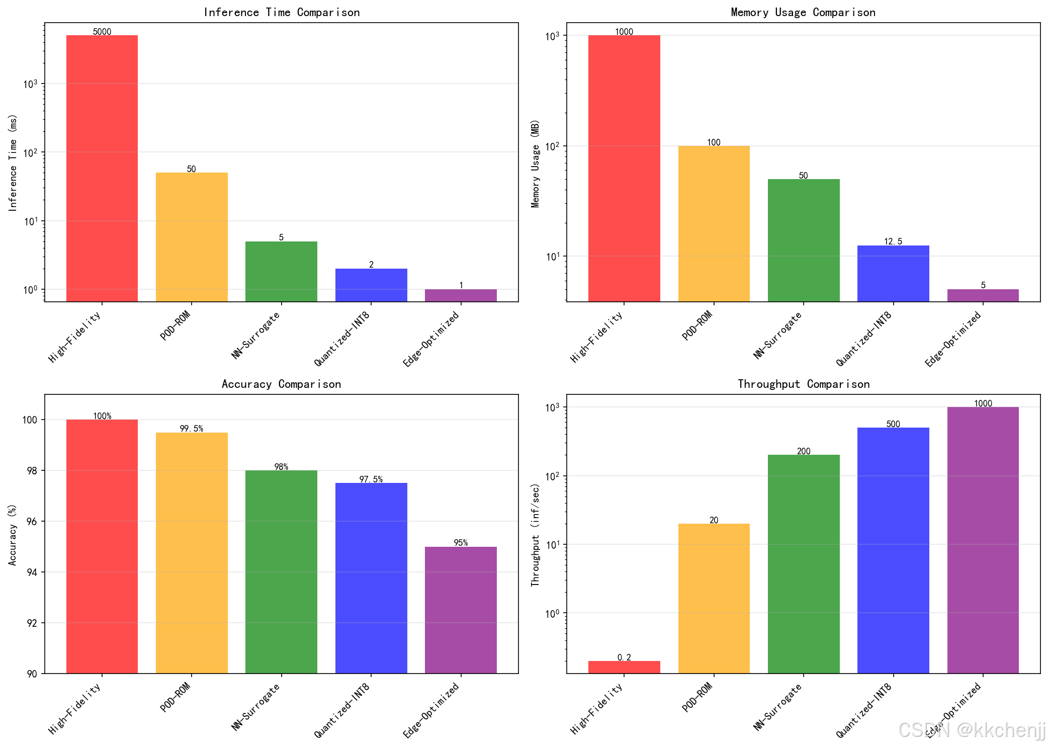
models = ['High-Fidelity', 'POD-ROM', 'NN-Surrogate', 'Quantized-INT8', 'Edge-Optimized']
# 性能数据(模拟)
inference_time = [5000, 50, 5, 2, 1] # ms
memory_usage = [1000, 100, 50, 12.5, 5] # MB
accuracy = [100, 99.5, 98, 97.5, 95] # %
throughput = [0.2, 20, 200, 500, 1000] # inferences/sec
print("\n性能对比:")
print(f"{'Model':<20} {'Time(ms)':<12} {'Memory(MB)':<12} {'Accuracy(%)':<12} {'Throughput':<12}")
print("-" * 70)
for i, model in enumerate(models):
print(f"{model:<20} {inference_time[i]:<12} {memory_usage[i]:<12} "
f"{accuracy[i]:<12} {throughput[i]:<12}")
# 可视化
fig, axes = plt.subplots(2, 2, figsize=(14, 10))
x = np.arange(len(models))
colors = ['red', 'orange', 'green', 'blue', 'purple']
# 推理时间对比
bars1 = axes[0, 0].bar(x, inference_time, color=colors, alpha=0.7)
axes[0, 0].set_yscale('log')
axes[0, 0].set_xticks(x)
axes[0, 0].set_xticklabels(models, rotation=45, ha='right')
axes[0, 0].set_ylabel('Inference Time (ms)')
axes[0, 0].set_title('Inference Time Comparison', fontsize=12)
axes[0, 0].grid(True, alpha=0.3, axis='y')
for bar, val in zip(bars1, inference_time):
axes[0, 0].text(bar.get_x() + bar.get_width()/2., bar.get_height(),
f'{val}', ha='center', va='bottom', fontsize=9)
# 内存使用对比
bars2 = axes[0, 1].bar(x, memory_usage, color=colors, alpha=0.7)
axes[0, 1].set_yscale('log')
axes[0, 1].set_xticks(x)
axes[0, 1].set_xticklabels(models, rotation=45, ha='right')
axes[0, 1].set_ylabel('Memory Usage (MB)')
axes[0, 1].set_title('Memory Usage Comparison', fontsize=12)
axes[0, 1].grid(True, alpha=0.3, axis='y')
for bar, val in zip(bars2, memory_usage):
axes[0, 1].text(bar.get_x() + bar.get_width()/2., bar.get_height(),
f'{val}', ha='center', va='bottom', fontsize=9)
# 准确率对比
bars3 = axes[1, 0].bar(x, accuracy, color=colors, alpha=0.7)
axes[1, 0].set_ylim([90, 101])
axes[1, 0].set_xticks(x)
axes[1, 0].set_xticklabels(models, rotation=45, ha='right')
axes[1, 0].set_ylabel('Accuracy (%)')
axes[1, 0].set_title('Accuracy Comparison', fontsize=12)
axes[1, 0].grid(True, alpha=0.3, axis='y')
for bar, val in zip(bars3, accuracy):
axes[1, 0].text(bar.get_x() + bar.get_width()/2., bar.get_height(),
f'{val}%', ha='center', va='bottom', fontsize=9)
# 吞吐量对比
bars4 = axes[1, 1].bar(x, throughput, color=colors, alpha=0.7)
axes[1, 1].set_yscale('log')
axes[1, 1].set_xticks(x)
axes[1, 1].set_xticklabels(models, rotation=45, ha='right')
axes[1, 1].set_ylabel('Throughput (inf/sec)')
axes[1, 1].set_title('Throughput Comparison', fontsize=12)
axes[1, 1].grid(True, alpha=0.3, axis='y')
for bar, val in zip(bars4, throughput):
axes[1, 1].text(bar.get_x() + bar.get_width()/2., bar.get_height(),
f'{val}', ha='center', va='bottom', fontsize=9)
plt.tight_layout()
plt.savefig('case9_performance_comparison.png', dpi=150, bbox_inches='tight')
print("\n结果已保存到 case9_performance_comparison.png")
plt.close()
return models, inference_time, accuracy
def create_summary_gif():
"""创建综合演示GIF动画"""
print("\n" + "="*60)
print("创建综合演示GIF动画")
print("="*60)
# 创建炉窑温控的简化动画
furnace = IndustrialFurnaceControl(nx=15, ny=15)
fig, axes = plt.subplots(1, 2, figsize=(12, 5))
# 初始化
im1 = axes[0].imshow(furnace.T, cmap='hot', vmin=800, vmax=1400)
axes[0].set_title('Real-time Temperature Field', fontsize=12)
axes[0].set_xlabel('x index')
axes[0].set_ylabel('y index')
plt.colorbar(im1, ax=axes[0], label='Temperature (K)')
line2, = axes[1].plot([], [], 'b-', linewidth=2)
axes[1].axhline(y=1200, color='r', linestyle='--', label='Target')
axes[1].set_xlim(0, 100)
axes[1].set_ylim(800, 1400)
axes[1].set_title('Temperature Control', fontsize=12)
axes[1].set_xlabel('Time (s)')
axes[1].set_ylabel('Average Temperature (K)')
axes[1].legend()
axes[1].grid(True, alpha=0.3)
mean_temps = []
times = []
def init():
im1.set_array(furnace.T)
line2.set_data([], [])
return [im1, line2]
def update(frame):
# 更新温度场
furnace.update_temperature(dt=0.5)
# 控制
if frame % 5 == 0:
furnace.control_loop(1200)
# 更新显示
im1.set_array(furnace.T)
mean_temps.append(np.mean(furnace.T))
times.append(frame * 0.5)
line2.set_data(times, mean_temps)
return [im1, line2]
print("生成GIF动画...")
anim = animation.FuncAnimation(fig, update, init_func=init,
frames=100, interval=100, blit=True)
anim.save('edge_computing_demo.gif', writer='pillow', fps=10)
print("动画已保存到 edge_computing_demo.gif")
plt.close()
def main():
"""主程序"""
print("\n" + "="*70)
print("主题090: 边缘计算中的辐射换热实时模拟")
print("="*70)
print("开始运行仿真案例...\n")
# 运行所有案例
try:
# 案例1: 高保真模型
model_hf, T_hf, I_hf = case1_high_fidelity_model()
# 案例2: POD降阶模型
pod_model, snapshots, params = case2_pod_reduced_model()
# 案例3: 神经网络代理模型
nn_model, nn_time = case3_neural_network_surrogate()
# 案例4: 模型量化
quant_model = case4_model_quantization()
# 案例5: 边缘-云端架构
architecture = case5_edge_cloud_architecture()
# 案例6: 实时数据处理
processor, stream_results = case6_realtime_data_processing()
# 案例7: 工业炉窑控制
furnace, T_history = case7_industrial_furnace_control()
# 案例8: 数据中心热管理
dc, dc_temps = case8_datacenter_thermal_management()
# 案例9: 性能对比
models, times, accs = case9_performance_comparison()
# 创建GIF动画
create_summary_gif()
print("\n" + "="*70)
print("所有案例运行完成!")
print("="*70)
print("\n生成的文件:")
print(" - case1_high_fidelity_model.png")
print(" - case2_pod_reduced_model.png")
print(" - case3_neural_network_surrogate.png")
print(" - case4_model_quantization.png")
print(" - case5_edge_cloud_architecture.png")
print(" - case6_realtime_data_processing.png")
print(" - case7_industrial_furnace_control.png")
print(" - case8_datacenter_thermal_management.png")
print(" - case9_performance_comparison.png")
print(" - edge_computing_demo.gif")
except Exception as e:
print(f"\n错误: {e}")
import traceback
traceback.print_exc()
if __name__ == "__main__":
main()

AtomGit 是由开放原子开源基金会联合 CSDN 等生态伙伴共同推出的新一代开源与人工智能协作平台。平台坚持“开放、中立、公益”的理念,把代码托管、模型共享、数据集托管、智能体开发体验和算力服务整合在一起,为开发者提供从开发、训练到部署的一站式体验。
更多推荐
 0
0 0
0- 0


 已为社区贡献264条内容

所有评论(0)