主题074_辐射热晶体管
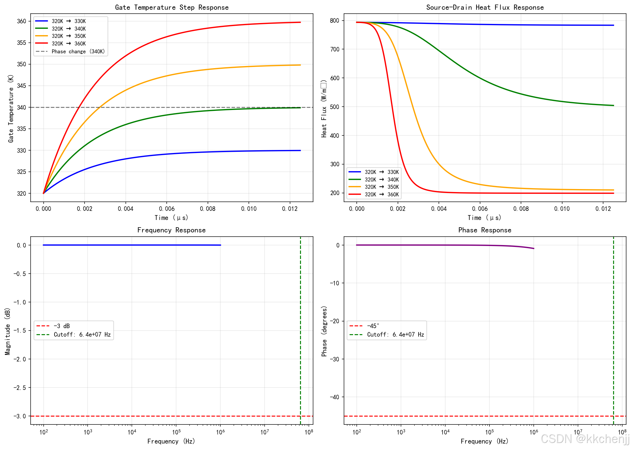
案例3:热晶体管动态响应仿真
本案例仿真热晶体管的动态响应特性,包括阶跃响应和频率响应。
import numpy as np
import matplotlib.pyplot as plt
from scipy.integrate import odeint

print("\n" + "=" * 70)
print("案例3:热晶体管动态响应仿真")
print("=" * 70)

# 物理常数
sigma = 5.67e-8
rho = 5000  # 密度 kg/m³
c_p = 500  # 比热容 J/(kg·K)
k = 10  # 热导率 W/(m·K)

# 热晶体管参数
T_s = 400  # 源极温度 (K)
T_d = 300  # 漏极温度 (K)
T_c = 340  # 相变温度 (K)

# 栅极参数
t_g = 100e-9  # 栅极厚度 (m)
A_g = 1e-6  # 栅极面积 (m²)
V_g = A_g * t_g  # 栅极体积

# 热容
C_th = rho * c_p * V_g  # J/K

# 热阻
R_th = t_g / (k * A_g)  # K/W

# 时间常数
tau = R_th * C_th

print(f"\n热晶体管动态参数:")
print(f"  栅极厚度: {t_g*1e9:.0f} nm")
print(f"  栅极面积: {A_g*1e6:.2f} mm²")
print(f"  热容: {C_th:.2e} J/K")
print(f"  热阻: {R_th:.2e} K/W")
print(f"  时间常数: {tau*1e6:.2f} μs")

# 阶跃响应仿真
def step_response(t, T_g_initial, T_g_final, tau):
    """栅极温度阶跃响应"""
    return T_g_final + (T_g_initial - T_g_final) * np.exp(-t / tau)

# 时间数组
t = np.linspace(0, 5*tau, 500)

# 不同阶跃幅度的响应
T_g_initial = 320
T_g_final_list = [330, 340, 350, 360]

fig, axes = plt.subplots(2, 2, figsize=(14, 10))

# 图1:栅极温度阶跃响应
ax1 = axes[0, 0]
colors = ['blue', 'green', 'orange', 'red']
for i, T_g_final in enumerate(T_g_final_list):
    T_g = step_response(t, T_g_initial, T_g_final, tau)
    ax1.plot(t*1e6, T_g, color=colors[i], linewidth=2,
             label=f'{T_g_initial}K → {T_g_final}K')

ax1.axhline(y=T_c, color='k', linestyle='--', alpha=0.5, label=f'Phase change ({T_c}K)')
ax1.set_xlabel('Time (μs)', fontsize=11)
ax1.set_ylabel('Gate Temperature (K)', fontsize=11)
ax1.set_title('Gate Temperature Step Response', fontsize=12, fontweight='bold')
ax1.legend(fontsize=9)
ax1.grid(True, alpha=0.3)

# 图2:源漏热流响应
def effective_emissivity(T_g, T_c):
    """有效发射率"""
    eps_ins = 0.8
    eps_met = 0.2
    delta_T = 5
    f = 0.5 * (1 + np.tanh((T_g - T_c) / delta_T))
    return eps_ins * (1 - f) + eps_met * f

ax2 = axes[0, 1]
for i, T_g_final in enumerate(T_g_final_list):
    T_g = step_response(t, T_g_initial, T_g_final, tau)
    eps_eff = effective_emissivity(T_g, T_c)
    Q_sd = eps_eff * sigma * (T_s**4 - T_d**4)
    ax2.plot(t*1e6, Q_sd, color=colors[i], linewidth=2,
             label=f'{T_g_initial}K → {T_g_final}K')

ax2.set_xlabel('Time (μs)', fontsize=11)
ax2.set_ylabel('Heat Flux (W/m²)', fontsize=11)
ax2.set_title('Source-Drain Heat Flux Response', fontsize=12, fontweight='bold')
ax2.legend(fontsize=9)
ax2.grid(True, alpha=0.3)

# 图3:频率响应
ax3 = axes[1, 0]
frequencies = np.logspace(2, 6, 100)  # Hz
omega = 2 * np.pi * frequencies

# 一阶系统频率响应
H = 1 / np.sqrt(1 + (omega * tau)**2)
phase = -np.arctan(omega * tau) * 180 / np.pi

ax3.semilogx(frequencies, 20*np.log10(H), 'b-', linewidth=2)
ax3.axhline(y=-3, color='r', linestyle='--', label='-3 dB')
f_c = 1 / (2 * np.pi * tau)
ax3.axvline(x=f_c, color='g', linestyle='--', label=f'Cutoff: {f_c:.1e} Hz')
ax3.set_xlabel('Frequency (Hz)', fontsize=11)
ax3.set_ylabel('Magnitude (dB)', fontsize=11)
ax3.set_title('Frequency Response', fontsize=12, fontweight='bold')
ax3.legend(fontsize=10)
ax3.grid(True, alpha=0.3)

# 图4:相位响应
ax4 = axes[1, 1]
ax4.semilogx(frequencies, phase, 'purple', linewidth=2)
ax4.axhline(y=-45, color='r', linestyle='--', label='-45°')
ax4.axvline(x=f_c, color='g', linestyle='--', label=f'Cutoff: {f_c:.1e} Hz')
ax4.set_xlabel('Frequency (Hz)', fontsize=11)
ax4.set_ylabel('Phase (degrees)', fontsize=11)
ax4.set_title('Phase Response', fontsize=12, fontweight='bold')
ax4.legend(fontsize=10)
ax4.grid(True, alpha=0.3)

plt.tight_layout()
plt.savefig('case3_dynamic_response.png', dpi=150)
plt.close()

print("\n结果已保存至: case3_dynamic_response.png")
print(f"\n截止频率: {f_c:.2e} Hz")
print("\n案例3完成!")
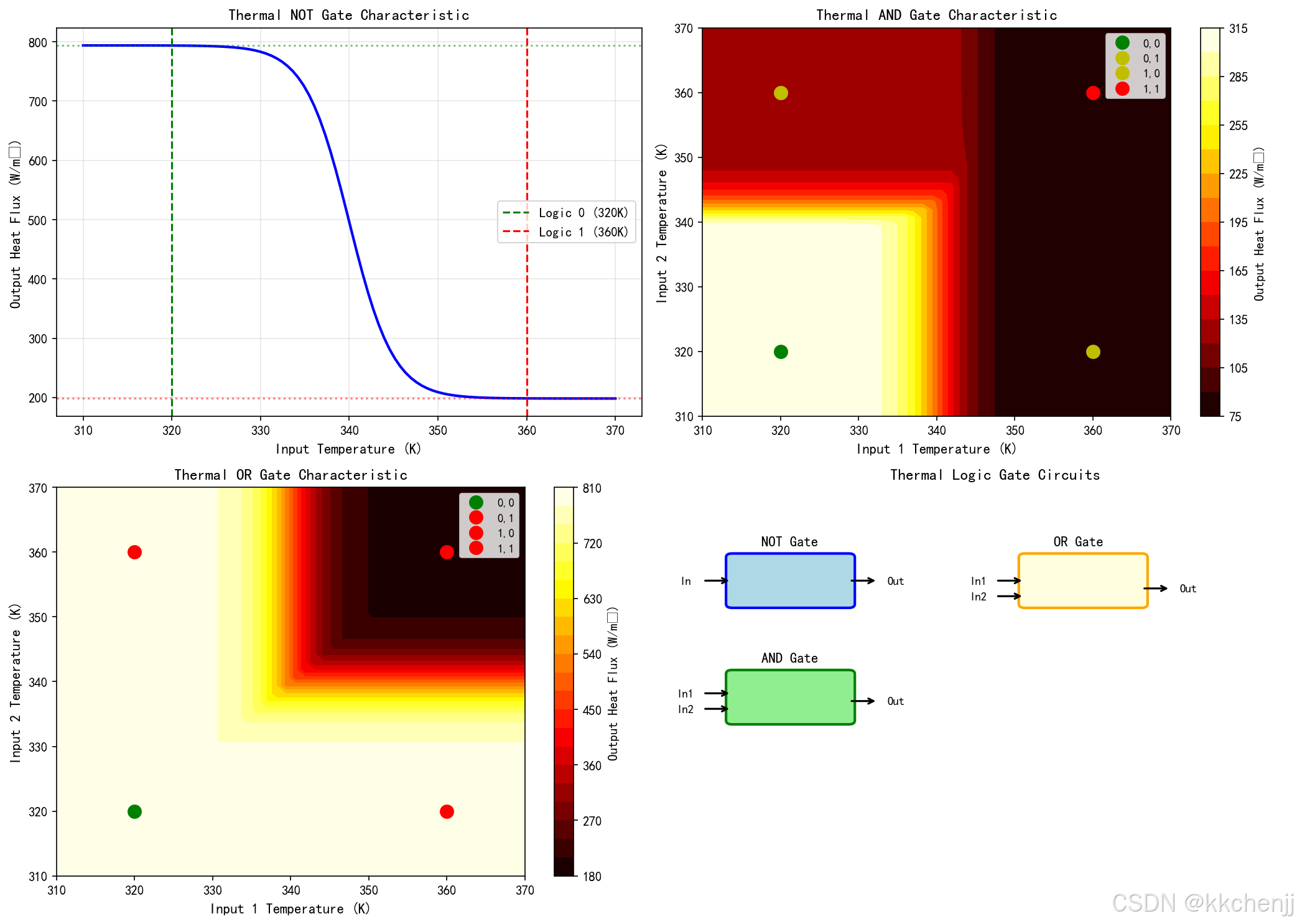
案例4:热逻辑门电路仿真
本案例仿真基于热晶体管的基本热逻辑门电路。
import numpy as np
import matplotlib.pyplot as plt
from matplotlib.patches import FancyBboxPatch, Circle, FancyArrowPatch

print("\n" + "=" * 70)
print("案例4:热逻辑门电路仿真")
print("=" * 70)

# 物理常数
sigma = 5.67e-8

# 热晶体管参数
T_s = 400  # 源极温度 (K)
T_d = 300  # 漏极温度 (K)
T_c = 340  # 相变温度 (K)
epsilon_ins = 0.8
epsilon_met = 0.2

def effective_emissivity(T_g, T_c):
    """有效发射率"""
    delta_T = 5
    f = 0.5 * (1 + np.tanh((T_g - T_c) / delta_T))
    return epsilon_ins * (1 - f) + epsilon_met * f

def thermal_transistor(T_g, T_s, T_d):
    """热晶体管模型"""
    eps_eff = effective_emissivity(T_g, T_c)
    return eps_eff * sigma * (T_s**4 - T_d**4)

# 热逻辑门仿真
print("\n热逻辑门仿真:")

# 输入温度(数字信号)
T_low = 320  # 逻辑0
T_high = 360  # 逻辑1

# 热非门(Thermal NOT)
def thermal_not(T_in):
    """热非门:高输入→低输出,低输入→高输出"""
    # 使用反相特性
    T_g = T_in
    Q_out = thermal_transistor(T_g, T_s, T_d)
    # 归一化到逻辑电平
    Q_max = thermal_transistor(T_low, T_s, T_d)
    Q_min = thermal_transistor(T_high, T_s, T_d)
    return Q_out, Q_max, Q_min

# 热与门(Thermal AND)
def thermal_and(T_in1, T_in2):
    """热与门:两个高输入→高输出"""
    # 串联结构:总热阻是两个晶体管热阻之和
    T_g1 = T_in1
    T_g2 = T_in2
    Q1 = thermal_transistor(T_g1, T_s, (T_s + T_d)/2)
    Q2 = thermal_transistor(T_g2, (T_s + T_d)/2, T_d)
    # 与门输出取最小值(串联限制)
    Q_out = min(Q1, Q2)
    return Q_out

# 热或门(Thermal OR)
def thermal_or(T_in1, T_in2):
    """热或门:任一高输入→高输出"""
    # 并联结构
    T_g1 = T_in1
    T_g2 = T_in2
    Q1 = thermal_transistor(T_g1, T_s, T_d)
    Q2 = thermal_transistor(T_g2, T_s, T_d)
    # 或门输出取最大值(并联增强)
    Q_out = max(Q1, Q2)
    return Q_out

# 真值表仿真
print("\n热非门真值表:")
print("  T_in (K)  |  Q_out (W/m²)  |  逻辑输出")
print("  " + "-" * 45)
for T_in in [T_low, T_high]:
    Q_out, Q_max, Q_min = thermal_not(T_in)
    logic_out = "0 (Low)" if Q_out < (Q_max + Q_min) / 2 else "1 (High)"
    print(f"  {T_in:3d}       |  {Q_out:11.2f}   |  {logic_out}")

print("\n热与门真值表:")
print("  T_in1 (K) | T_in2 (K) | Q_out (W/m²) | 逻辑输出")
print("  " + "-" * 55)
for T_in1 in [T_low, T_high]:
    for T_in2 in [T_low, T_high]:
        Q_out = thermal_and(T_in1, T_in2)
        Q_ref = thermal_transistor(T_low, T_s, T_d)
        logic_out = "0 (Low)" if Q_out < Q_ref * 0.8 else "1 (High)"
        print(f"  {T_in1:3d}       | {T_in2:3d}       | {Q_out:11.2f}  | {logic_out}")

print("\n热或门真值表:")
print("  T_in1 (K) | T_in2 (K) | Q_out (W/m²) | 逻辑输出")
print("  " + "-" * 55)
for T_in1 in [T_low, T_high]:
    for T_in2 in [T_low, T_high]:
        Q_out = thermal_or(T_in1, T_in2)
        Q_ref = thermal_transistor(T_high, T_s, T_d)
        logic_out = "1 (High)" if Q_out > Q_ref * 0.2 else "0 (Low)"
        print(f"  {T_in1:3d}       | {T_in2:3d}       | {Q_out:11.2f}  | {logic_out}")

# 绘图
fig, axes = plt.subplots(2, 2, figsize=(14, 10))

# 图1:热非门特性
ax1 = axes[0, 0]
T_in_range = np.linspace(310, 370, 100)
Q_out_range = [thermal_transistor(T, T_s, T_d) for T in T_in_range]
ax1.plot(T_in_range, Q_out_range, 'b-', linewidth=2)
ax1.axvline(x=T_low, color='g', linestyle='--', label=f'Logic 0 ({T_low}K)')
ax1.axvline(x=T_high, color='r', linestyle='--', label=f'Logic 1 ({T_high}K)')
ax1.axhline(y=thermal_transistor(T_low, T_s, T_d), color='g', linestyle=':', alpha=0.5)
ax1.axhline(y=thermal_transistor(T_high, T_s, T_d), color='r', linestyle=':', alpha=0.5)
ax1.set_xlabel('Input Temperature (K)', fontsize=11)
ax1.set_ylabel('Output Heat Flux (W/m²)', fontsize=11)
ax1.set_title('Thermal NOT Gate Characteristic', fontsize=12, fontweight='bold')
ax1.legend(fontsize=10)
ax1.grid(True, alpha=0.3)

# 图2:热与门特性
ax2 = axes[0, 1]
T_range = np.linspace(310, 370, 50)
Q_and = np.zeros((50, 50))
for i, T1 in enumerate(T_range):
    for j, T2 in enumerate(T_range):
        Q_and[i, j] = thermal_and(T1, T2)

im = ax2.contourf(T_range, T_range, Q_and, levels=20, cmap='hot')
plt.colorbar(im, ax=ax2, label='Output Heat Flux (W/m²)')
ax2.set_xlabel('Input 1 Temperature (K)', fontsize=11)
ax2.set_ylabel('Input 2 Temperature (K)', fontsize=11)
ax2.set_title('Thermal AND Gate Characteristic', fontsize=12, fontweight='bold')

# 标记逻辑电平
ax2.plot(T_low, T_low, 'go', markersize=10, label='0,0')
ax2.plot(T_low, T_high, 'yo', markersize=10, label='0,1')
ax2.plot(T_high, T_low, 'yo', markersize=10, label='1,0')
ax2.plot(T_high, T_high, 'ro', markersize=10, label='1,1')
ax2.legend(fontsize=9)

# 图3:热或门特性
ax3 = axes[1, 0]
Q_or = np.zeros((50, 50))
for i, T1 in enumerate(T_range):
    for j, T2 in enumerate(T_range):
        Q_or[i, j] = thermal_or(T1, T2)

im = ax3.contourf(T_range, T_range, Q_or, levels=20, cmap='hot')
plt.colorbar(im, ax=ax3, label='Output Heat Flux (W/m²)')
ax3.set_xlabel('Input 1 Temperature (K)', fontsize=11)
ax3.set_ylabel('Input 2 Temperature (K)', fontsize=11)
ax3.set_title('Thermal OR Gate Characteristic', fontsize=12, fontweight='bold')

# 标记逻辑电平
ax3.plot(T_low, T_low, 'go', markersize=10, label='0,0')
ax3.plot(T_low, T_high, 'ro', markersize=10, label='0,1')
ax3.plot(T_high, T_low, 'ro', markersize=10, label='1,0')
ax3.plot(T_high, T_high, 'ro', markersize=10, label='1,1')
ax3.legend(fontsize=9)

# 图4:逻辑门电路示意图
ax4 = axes[1, 1]
ax4.set_xlim(0, 10)
ax4.set_ylim(0, 10)
ax4.axis('off')

# NOT门
ax4.text(1, 8.5, 'NOT Gate', fontsize=11, fontweight='bold')
not_gate = FancyBboxPatch((0.5, 7), 2, 1.2, boxstyle="round,pad=0.1",
                          facecolor='lightblue', edgecolor='blue', linewidth=2)
ax4.add_patch(not_gate)
ax4.annotate('', xy=(0.5, 7.6), xytext=(0, 7.6),
            arrowprops=dict(arrowstyle='->', color='black', lw=1.5))
ax4.text(-0.3, 7.6, 'In', fontsize=9, ha='center', va='center')
ax4.annotate('', xy=(3, 7.6), xytext=(2.5, 7.6),
            arrowprops=dict(arrowstyle='->', color='black', lw=1.5))
ax4.text(3.3, 7.6, 'Out', fontsize=9, ha='center', va='center')

# AND门
ax4.text(1, 5.5, 'AND Gate', fontsize=11, fontweight='bold')
and_gate = FancyBboxPatch((0.5, 4), 2, 1.2, boxstyle="round,pad=0.1",
                          facecolor='lightgreen', edgecolor='green', linewidth=2)
ax4.add_patch(and_gate)
ax4.annotate('', xy=(0.5, 4.7), xytext=(0, 4.7),
            arrowprops=dict(arrowstyle='->', color='black', lw=1.5))
ax4.text(-0.3, 4.7, 'In1', fontsize=9, ha='center', va='center')
ax4.annotate('', xy=(0.5, 4.3), xytext=(0, 4.3),
            arrowprops=dict(arrowstyle='->', color='black', lw=1.5))
ax4.text(-0.3, 4.3, 'In2', fontsize=9, ha='center', va='center')
ax4.annotate('', xy=(3, 4.5), xytext=(2.5, 4.5),
            arrowprops=dict(arrowstyle='->', color='black', lw=1.5))
ax4.text(3.3, 4.5, 'Out', fontsize=9, ha='center', va='center')

# OR门
ax4.text(6, 8.5, 'OR Gate', fontsize=11, fontweight='bold')
or_gate = FancyBboxPatch((5.5, 7), 2, 1.2, boxstyle="round,pad=0.1",
                         facecolor='lightyellow', edgecolor='orange', linewidth=2)
ax4.add_patch(or_gate)
ax4.annotate('', xy=(5.5, 4.7), xytext=(5, 4.7),
            arrowprops=dict(arrowstyle='->', color='black', lw=1.5))
ax4.text(4.7, 4.7, 'In1', fontsize=9, ha='center', va='center')
ax4.annotate('', xy=(5.5, 4.3), xytext=(5, 4.3),
            arrowprops=dict(arrowstyle='->', color='black', lw=1.5))
ax4.text(4.7, 4.3, 'In2', fontsize=9, ha='center', va='center')
ax4.annotate('', xy=(8, 4.5), xytext=(7.5, 4.5),
            arrowprops=dict(arrowstyle='->', color='black', lw=1.5))
ax4.text(8.3, 4.5, 'Out', fontsize=9, ha='center', va='center')

ax4.set_title('Thermal Logic Gate Circuits', fontsize=12, fontweight='bold')

plt.tight_layout()
plt.savefig('case4_thermal_logic.png', dpi=150)
plt.close()

print("\n结果已保存至: case4_thermal_logic.png")
print("\n案例4完成!")
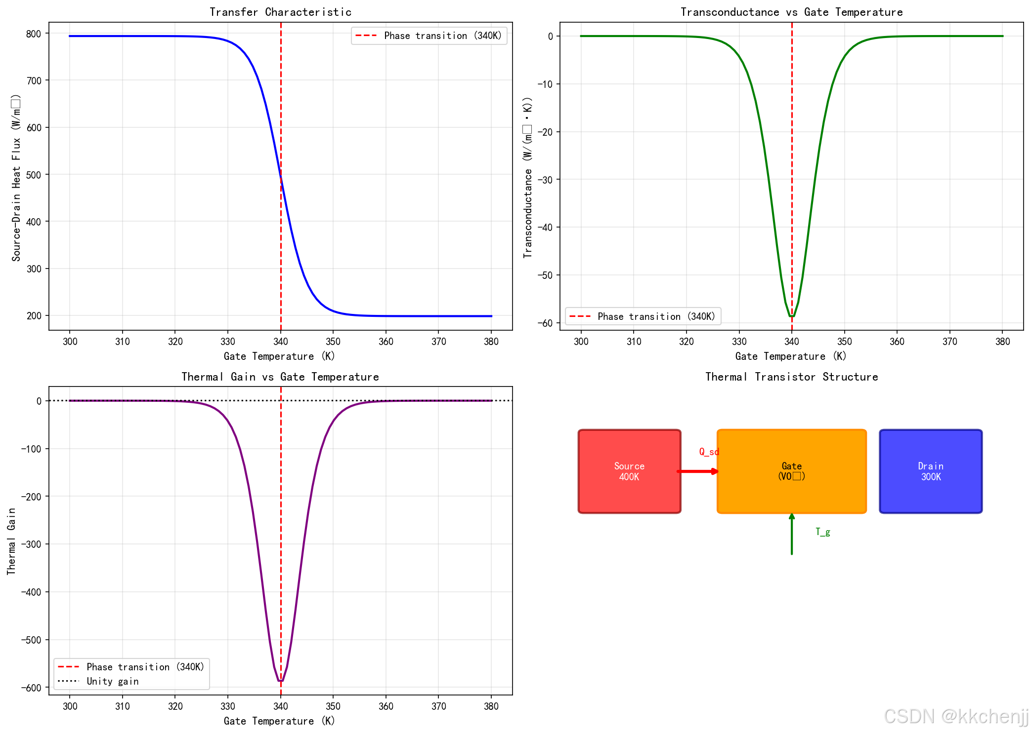
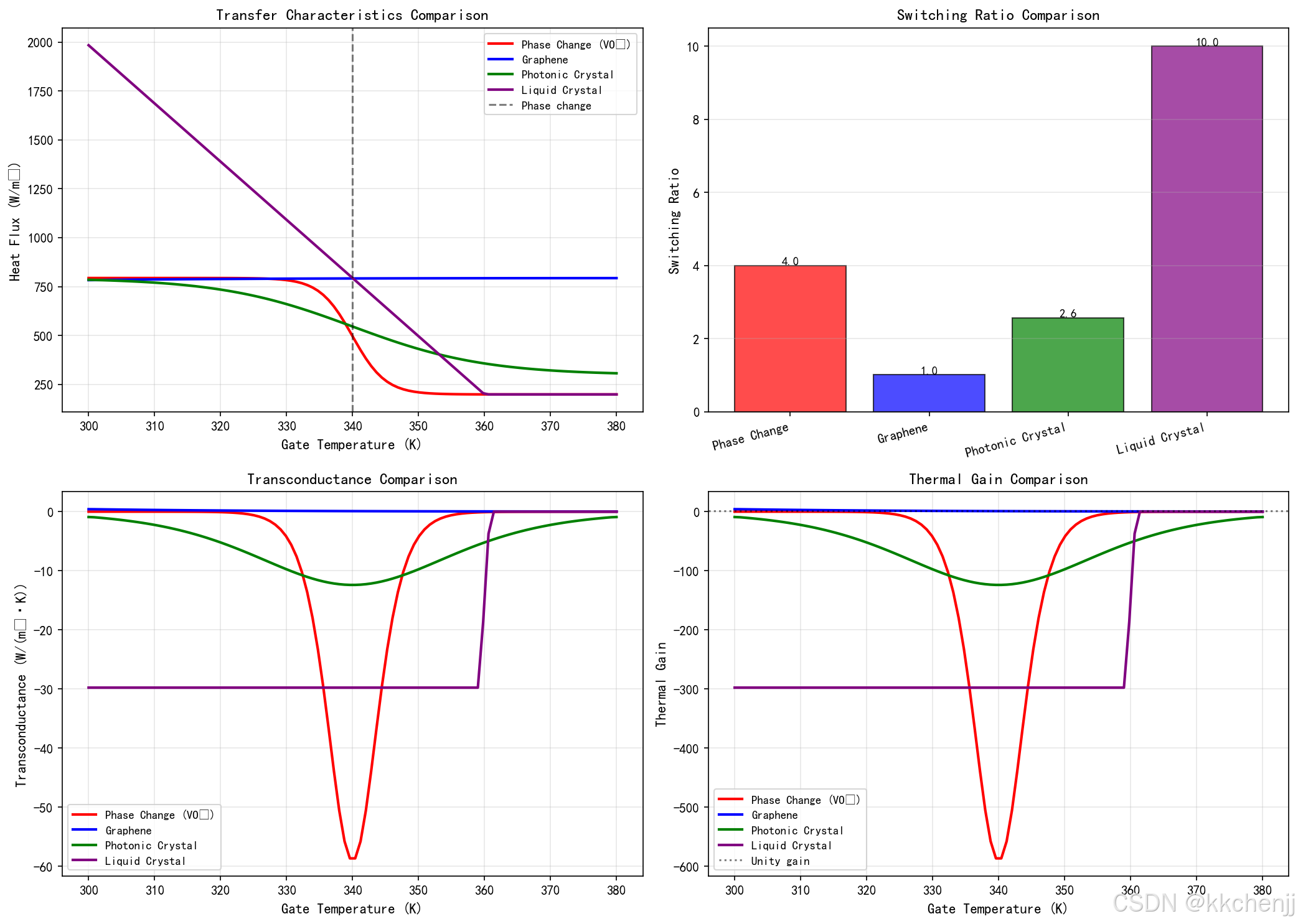
案例5:热晶体管性能对比与优化
本案例对比不同类型热晶体管的性能,并探讨优化策略。
import numpy as np
import matplotlib.pyplot as plt

print("\n" + "=" * 70)
print("案例5:热晶体管性能对比与优化")
print("=" * 70)

# 物理常数
sigma = 5.67e-8

# 基础温度
T_s = 400  # K
T_d = 300  # K

# 定义不同类型的热晶体管

def phase_change_transistor(T_g, T_c=340, eps_ins=0.8, eps_met=0.2):
    """相变材料热晶体管(VO2)"""
    delta_T = 5
    f = 0.5 * (1 + np.tanh((T_g - T_c) / delta_T))
    eps_eff = eps_ins * (1 - f) + eps_met * f
    return eps_eff * sigma * (T_s**4 - T_d**4)

def graphene_transistor(T_g, T_c=340):
    """石墨烯热晶体管"""
    # 石墨烯费米能级随温度变化
    E_f = 0.1 + 0.001 * (T_g - 300)  # eV
    # 发射率随费米能级变化
    eps_eff = 0.5 + 0.3 * np.tanh(E_f / 0.05)
    return eps_eff * sigma * (T_s**4 - T_d**4)

def photonic_crystal_transistor(T_g, T_c=340):
    """光子晶体热晶体管"""
    # 带边随温度移动
    band_edge_shift = 0.01 * (T_g - T_c)  # μm
    # 透射率变化
    T_trans = 0.3 + 0.5 / (1 + np.exp(band_edge_shift / 0.1))
    return T_trans * sigma * (T_s**4 - T_d**4)

def liquid_crystal_transistor(T_g, T_c=340):
    """液晶热晶体管"""
    # 液晶取向随温度变化
    order_param = np.maximum(0, 1 - (T_g - T_c) / 20)
    # 双折射变化导致透射率变化
    T_trans = 0.2 + 0.6 * order_param
    return T_trans * sigma * (T_s**4 - T_d**4)

# 温度范围
T_g_range = np.linspace(300, 380, 100)

# 计算各类热晶体管的热流
transistors = {
    'Phase Change (VO₂)': {'func': phase_change_transistor, 'color': 'red'},
    'Graphene': {'func': graphene_transistor, 'color': 'blue'},
    'Photonic Crystal': {'func': photonic_crystal_transistor, 'color': 'green'},
    'Liquid Crystal': {'func': liquid_crystal_transistor, 'color': 'purple'}
}

results = {}
for name, params in transistors.items():
    Q_sd = [params['func'](T_g) for T_g in T_g_range]
    results[name] = {
        'Q_sd': np.array(Q_sd),
        'color': params['color']
    }

# 计算性能指标
print("\n热晶体管性能对比:")
print("=" * 70)
print(f"{'Type':<25} {'Q_max':<12} {'Q_min':<12} {'Ratio':<10} {'Max dQ/dT':<12}")
print("-" * 70)

for name, data in results.items():
    Q_max = np.max(data['Q_sd'])
    Q_min = np.min(data['Q_sd'])
    ratio = Q_max / Q_min if Q_min > 0 else float('inf')
    dQ_dT = np.max(np.gradient(data['Q_sd'], T_g_range))
    print(f"{name:<25} {Q_max:<12.2f} {Q_min:<12.2f} {ratio:<10.2f} {dQ_dT:<12.4f}")

# 计算热增益(假设栅极热阻为10 K/W)
R_g = 10  # K/W
print("\n热增益对比(R_g = 10 K/W):")
print("-" * 50)
for name, data in results.items():
    g_m = np.gradient(data['Q_sd'], T_g_range)
    G = g_m * R_g
    G_max = np.max(G)
    print(f"{name:<25} G_max = {G_max:.2f}")

# 绘图
fig, axes = plt.subplots(2, 2, figsize=(14, 10))

# 图1:各类热晶体管转移特性
ax1 = axes[0, 0]
for name, data in results.items():
    ax1.plot(T_g_range, data['Q_sd'], color=data['color'],
             linewidth=2, label=name)
ax1.axvline(x=340, color='k', linestyle='--', alpha=0.5, label='Phase change')
ax1.set_xlabel('Gate Temperature (K)', fontsize=11)
ax1.set_ylabel('Heat Flux (W/m²)', fontsize=11)
ax1.set_title('Transfer Characteristics Comparison', fontsize=12, fontweight='bold')
ax1.legend(fontsize=9)
ax1.grid(True, alpha=0.3)

# 图2:开关比对比
ax2 = axes[0, 1]
names = list(results.keys())
ratios = []
for name, data in results.items():
    Q_max = np.max(data['Q_sd'])
    Q_min = np.min(data['Q_sd'])
    ratios.append(Q_max / Q_min if Q_min > 0 else 0)

colors = [results[name]['color'] for name in names]
bars = ax2.bar(range(len(names)), ratios, color=colors, alpha=0.7, edgecolor='black')
ax2.set_xticks(range(len(names)))
ax2.set_xticklabels([n.split('(')[0].strip() for n in names], rotation=15, ha='right')
ax2.set_ylabel('Switching Ratio', fontsize=11)
ax2.set_title('Switching Ratio Comparison', fontsize=12, fontweight='bold')
ax2.grid(True, alpha=0.3, axis='y')

# 添加数值标签
for bar, ratio in zip(bars, ratios):
    height = bar.get_height()
    ax2.text(bar.get_x() + bar.get_width()/2., height,
             f'{ratio:.1f}', ha='center', va='bottom', fontsize=9)

# 图3:跨导热导对比
ax3 = axes[1, 0]
for name, data in results.items():
    g_m = np.gradient(data['Q_sd'], T_g_range)
    ax3.plot(T_g_range, g_m, color=data['color'],
             linewidth=2, label=name)
ax3.set_xlabel('Gate Temperature (K)', fontsize=11)
ax3.set_ylabel('Transconductance (W/(m²·K))', fontsize=11)
ax3.set_title('Transconductance Comparison', fontsize=12, fontweight='bold')
ax3.legend(fontsize=9)
ax3.grid(True, alpha=0.3)

# 图4:热增益对比
ax4 = axes[1, 1]
for name, data in results.items():
    g_m = np.gradient(data['Q_sd'], T_g_range)
    G = g_m * R_g
    ax4.plot(T_g_range, G, color=data['color'],
             linewidth=2, label=name)
ax4.axhline(y=1, color='k', linestyle=':', alpha=0.5, label='Unity gain')
ax4.set_xlabel('Gate Temperature (K)', fontsize=11)
ax4.set_ylabel('Thermal Gain', fontsize=11)
ax4.set_title('Thermal Gain Comparison', fontsize=12, fontweight='bold')
ax4.legend(fontsize=9)
ax4.grid(True, alpha=0.3)

plt.tight_layout()
plt.savefig('case5_performance_comparison.png', dpi=150)
plt.close()

print("\n结果已保存至: case5_performance_comparison.png")
print("\n案例5完成!")

print("\n" + "=" * 70)
print("所有仿真案例已完成!")
print("=" * 70)
8. 总结与展望
8.1 核心要点总结
本教程系统介绍了辐射热晶体管的基本概念、工作原理、理论模型、设计方法和应用场景。核心要点包括:
1. 基本概念
- 辐射热晶体管是一种三端热管理器件,通过栅极控制源漏之间的辐射热流
- 类比于电子晶体管,可以实现热流的放大和开关控制
- 具有非接触、快速响应、纳米尺度适用等独特优势
2. 工作原理
- 热增益 G=ΔQsd/ΔQgG = \Delta Q_{sd} / \Delta Q_gG=ΔQsd/ΔQg 是核心性能指标
- 热放大依赖于温度依赖的辐射特性、近场耦合调制和相变效应
- 开关比 Rsw=Qsdon/QsdoffR_{sw} = Q_{sd}^{on} / Q_{sd}^{off}Rsw=Qsdon/Qsdoff 表征开关性能
3. 理论模型
- 近场辐射模型:利用涨落耗散定理计算纳米尺度热流
- 相变材料模型:利用VO₂等材料的相变特性实现热开关
- 光子晶体模型:利用带隙调控实现光谱选择性热控制
- 热电路模型:便于电路分析和系统集成
4. 设计实现
- 材料选择:源漏极(金属、极性介质)、栅极(相变材料、石墨烯、液晶)
- 结构优化:间隙距离、栅极厚度、光谱匹配
- 制造工艺:薄膜沉积、纳米加工、间隙控制
5. 性能表征
- 静态特性:输入特性、输出特性、转移特性
- 动态特性:阶跃响应、频率响应、开关速度
- 性能指标:热增益、开关比、跨导热导、截止频率
6. 应用场景
- 热逻辑运算:NOT、AND、OR等基本逻辑门
- 热计算:模拟计算、数字计算、热神经网络
- 热管理:智能热开关、热流放大器、热振荡器
- 能量转换:热光伏优化、热回收、辐射制冷控制
8.2 技术挑战与解决方案
辐射热晶体管面临的主要技术挑战包括:
1. 热增益提升
- 挑战:目前热增益通常小于10,难以满足实际应用需求
- 解决方案:采用高灵敏度相变材料、优化栅极热阻、利用共振增强效应、级联多个晶体管
2. 开关比提高
- 挑战:开关比受限于材料性质对比度和结构非对称性
- 解决方案:利用相变突变、设计高对比度光子带隙、采用多层结构
3. 响应速度优化
- 挑战:热响应速度受限于热容和热阻
- 解决方案:薄膜化、纳米结构化、采用高导热材料、优化热路设计
4. 工作温度降低
- 挑战:许多相变材料的工作温度较高(如VO₂为68°C)
- 解决方案:开发低温相变材料、利用量子限制效应、应力调控
5. 制造与集成
- 挑战:纳米尺度间隙的控制和大面积制造
- 解决方案:自组装技术、纳米压印、MEMS工艺、柔性转移技术
8.3 未来发展趋势
辐射热晶体管作为新兴的热管理技术,未来发展趋势包括:
1. 新材料探索
- 二维材料(石墨烯、氮化硼、过渡金属硫化物)
- 拓扑材料
- 钙钛矿相变材料
- 智能响应材料(水凝胶、形状记忆合金)
2. 新结构设计
- 超表面和超材料结构
- 非互易热辐射结构
- 动态可调结构
- 三维集成结构
3. 多功能集成
- 热-电协同调控
- 热-光协同调控
- 热-机械协同调控
- 多物理场耦合器件
4. 系统级应用
- 热逻辑处理器
- 热神经网络芯片
- 智能热管理系统
- 热通信系统
5. 极端环境应用
- 航天器智能热控
- 核反应堆热管理
- 高温电子器件冷却
- 极地/沙漠环境应用
8.4 研究前沿
当前辐射热晶体管的研究前沿包括:
1. 量子热晶体管
利用量子效应(如量子点、量子阱)实现热流的量子调控,探索量子热力学极限。
2. 拓扑热晶体管
利用拓扑保护的边缘态实现鲁棒的热传输调控,提高器件的稳定性和可靠性。
3. 非互易热晶体管
结合热二极管和热晶体管功能,实现单向热流放大和开关控制。
4. 可重构热晶体管
通过外部场(电场、磁场、光场)动态重构热晶体管特性,实现可编程热管理。
5. 生物启发设计
从生物系统(如人体温度调节、植物蒸腾作用)获取灵感,设计自适应热管理器件。
8.5 结语
辐射热晶体管代表了热管理技术的范式转变,从被动散热向主动热控制演进。虽然目前仍处于研究阶段,但其在热计算、智能热管理、能量转换等领域展现出的巨大潜力,使其成为热科学和工程领域的前沿热点。
随着纳米技术、材料科学和计算方法的进步,辐射热晶体管的性能将不断提升,应用场景将不断拓展。未来,我们有望看到基于热晶体管的热逻辑处理器、智能热管理系统和热神经网络等创新应用,为能源、信息、航天等领域带来革命性的技术变革。
热,作为能量最基本的形式之一,其精确控制一直是人类追求的目标。辐射热晶体管的出现,为我们提供了一种全新的热控制范式,开启了"热电子学"的新篇章。让我们期待这一前沿技术的持续突破和广泛应用,为构建更高效、更智能、更可持续的热管理系统贡献力量。

AtomGit 是由开放原子开源基金会联合 CSDN 等生态伙伴共同推出的新一代开源与人工智能协作平台。平台坚持“开放、中立、公益”的理念,把代码托管、模型共享、数据集托管、智能体开发体验和算力服务整合在一起,为开发者提供从开发、训练到部署的一站式体验。
更多推荐

 0
0 0
0- 0


 已为社区贡献273条内容

所有评论(0)