示波器traces采集
业务上遇到一个示波器traces采集的问题,他们用的采集脚本是好几年前的开源脚本,一直没有更新和维护,跟新的示波器不匹配,第一步通讯就卡住了,然后把问题抛给我。我对示波器的了解仅限于当年在大学实验课上接触过,并没有过多的了解,这次就当学习了。
方案选择
他们原本是想让我在以前的脚本上做修改,但我打开那个开源仓库,上次更新时间是在7.8年前,对于示波器都还不了解,一上来就让我改工具,未免有点为难我,还是另寻他法。
首先弄清楚示波器的型号,是 PICO3000E系列的。
搜索一圈下来,发现 pico 官方是有提供软件和SDK的,这样可以直接用官方的接口,然后再改写脚本到我们希望看到的效果就好了。
具体怎么操作,官方有提供教程:PyPicoSDK: Getting Started
环境搭建
这里跟着官方的教程走就可以。
1. 安装 PicoSDK
下载地址:https://www.picotech.com/downloads
选择具体示波器型号和系统对应的安装包就可以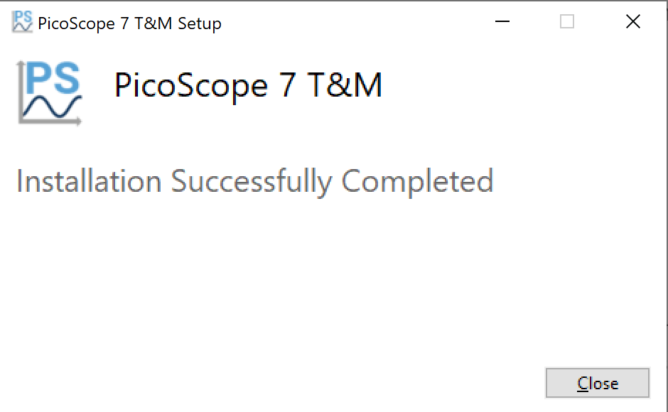
2. 安装需要的 python 库
pip install pypicosdk
pip install matplotlib
pip install scipy
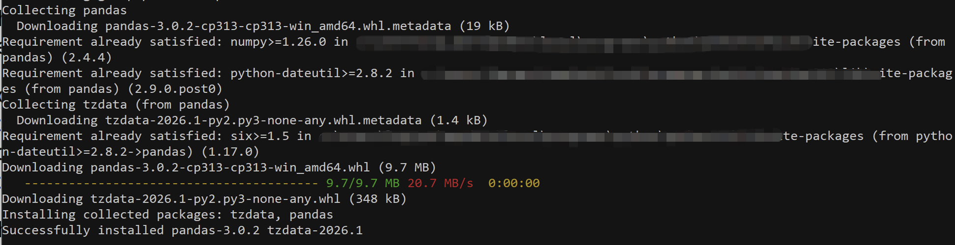
pip install pandas
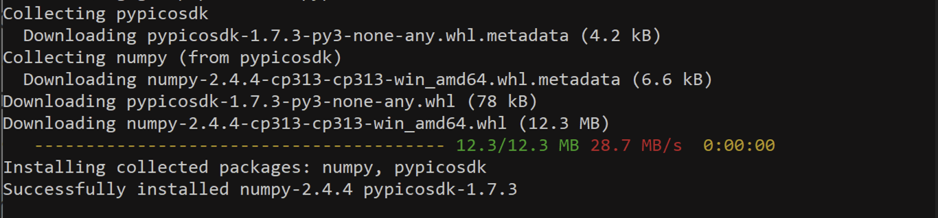
安装 pypicosdk :
(可以看到结果,在这个过程 numpy 同时也被安装了)
安装 matplotlib :
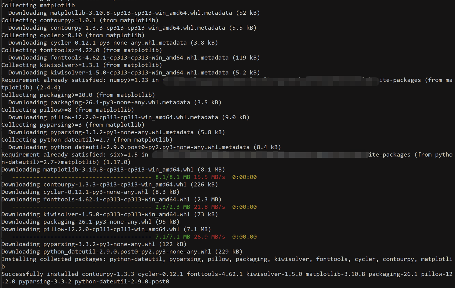
安装 scipy :

安装 pandas :
编写脚本
在官方的仓库里,有提供挺多 example 可以参考的,可以在这个基础上加细节适配采集需求
官方仓库示例:examples
1. 验证示波器存在
用官方示例 enumerate_units.py 验证测试电脑能找到示波器,确保第一步成功
"""
Copyright (C) 2025-2025 Pico Technology Ltd. See LICENSE file for terms.

This example enumerates all PicoScope units (supported by pyPicoSDK), returns the number
of units and a list of serial numbers.
"""

import pypicosdk as psdk

# Enumerate units
n_units, units = psdk.get_all_enumerated_units()

# Print output
print(f'Number of units: {n_units}')
for unit, serial in units.items():
    print(f'{unit}: {serial}')
运行结果:

2. 适配采集需求
在需求的测试场景中,第一是要采集大量的traces用于后续分析,第二是要能够采集到触发的完整波形。
也就是需要解决波形问题,还有数据量的问题。
2.1 调整波形
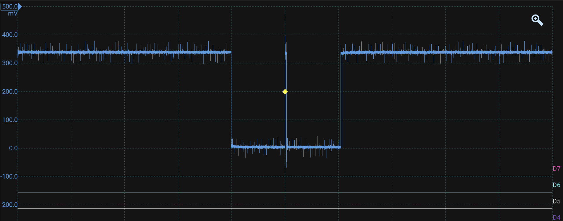
首先是要配置好采集通道和触发条件。这个可以先打开上面安装的 PicoScope 7 T&M 这个工具,因为是图形界面,操作起来比脚本简单快速,也很直观。所以先用它调好参数,然后再把参数填到脚本中即可。
这是调好的波形:
2.2 编写脚本
是在官方 simple_block_capture.py 这个脚本的基础上去改的。
import pypicosdk as psdk
import numpy as np
import matplotlib.pyplot as plt
import time
import os
from datetime import datetime

# ============================================================
# User-adjustable parameters (modify according to your chip signal)
# ============================================================
CHANNEL = psdk.CHANNEL.A                      # Channel where the probe is connected
VOLTAGE_RANGE = psdk.RANGE.mV500  # Voltage range, match your chip's output level
COUPLING = psdk.COUPLING.DC                    # Coupling mode (usually DC for digital circuits)
TRIGGER_CHANNEL = psdk.CHANNEL.A              # Trigger source channel
TRIGGER_THRESHOLD = 200            # Trigger level in volts
TRIGGER_DIRECTION = psdk.TRIGGER_DIR.RISING       # Trigger on rising edge
TIMEBASE = 1000000                    # Sample interval in seconds (1e-6 = 1 us, 1 MS/s)
# sample_rate = 9_765_625
TOTAL_SAMPLES = 5000                # Total number of samples per capture
TOTAL_CAPTURES = 10
# PRE_TRIG_PERCENT = 10          # Samples to keep before the trigger point
# POST_TRIGGER_SAMPLES = NUM_SAMPLES - PRE_TRIGGER_SAMPLES  # Samples after trigger

SAVE_DIR = "./captured_traces"
os.makedirs(SAVE_DIR, exist_ok=True)

# ============================================================
# 1. Connect to the oscilloscope (PicoScope 3000E uses psospa class)
# ============================================================
print("Connecting to PicoScope...")
scope = psdk.psospa()
scope.open_unit()
print("Scope connected.")

# Optional: print some device information
try:
    driver_info = scope.get_unit_serial()
    print(f"device info: {driver_info}")
except:
    pass

# ============================================================
# 2. Configure the input channel
# ============================================================
print("Configuring channel...\n")
scope.set_channel(CHANNEL, enabled=True, coupling=COUPLING, range=VOLTAGE_RANGE)
print("set channel success...\n")

# Disable other channels to save resources
# for ch in ["B", "C", "D"]:
#     try:
#         scope.set_channel(ch, enabled=False)
#     except:
#         pass

# ============================================================
# 3. Set up the trigger (external chip signal, no auto-trigger)
# ============================================================
print("Setting trigger...")
scope.set_simple_trigger(
    TRIGGER_CHANNEL,
    threshold=TRIGGER_THRESHOLD,
    direction=TRIGGER_DIRECTION,
    auto_trigger=0   # Disable auto-trigger; wait for a real signal edge
)
print(f"Waiting for trigger on Channel {TRIGGER_CHANNEL} "
      f"({TRIGGER_DIRECTION}, {TRIGGER_THRESHOLD}mV)...")

# Perform simple block capture via help function (inc. buffer setup, time axis, mV conversion etc.)
# timebase = scope.sample_rate_to_timebase(sample_rate=sample_rate)
# print(f"Calculated timebase: {timebase}")
channel_buffer, time_axis = scope.run_simple_block_capture(TIMEBASE, TOTAL_SAMPLES,time_unit="ms")
print(f"time_axis: {time_axis}")
# channel_buffers, time_axis = scope.run_simple_rapid_block_capture(TIMEBASE, TOTAL_SAMPLES, TOTAL_CAPTURES)

# all_traces = channel_buffers[psdk.CHANNEL.A]

# timestamp = datetime.now().strftime("%Y%m%d_%H%M%S")
# filename = f"./captured_traces/traces_{TOTAL_CAPTURES}_{timestamp}.npy"

# np.save(filename, all_traces)
# print(f"Saved {TOTAL_CAPTURES} tarces to {filename}")

# Release the device from the driver
scope.close_unit()

# # Use matplotlib to setup the graph and plot the data
plt.figure(figsize=(13, 5))
plt.plot(time_axis, channel_buffer[psdk.CHANNEL.A])
# for trace in all_traces:
#     plt.plot(time_axis, trace)
# plt.plot(time_axis, all_traces[0])

plt.xlabel("Time (ms)")
plt.ylabel("Amplitude (mV)")
plt.grid(True)
plt.show()
(因为后续是要采集大量traces的,这里只展示采集单个波形,所以脚本显得注释掉的很多,当时也是不断的在调,修修改改,不停的看效果,然后再优化)
看下没调对触发条件是怎样的:
只有噪声,没有触发事件。
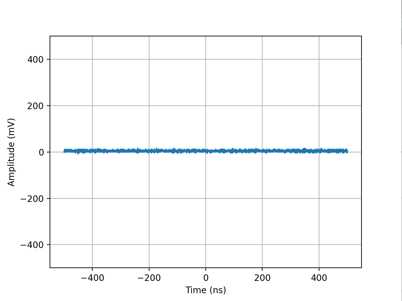
调对了trigger ,但是波形只能采集到一半。
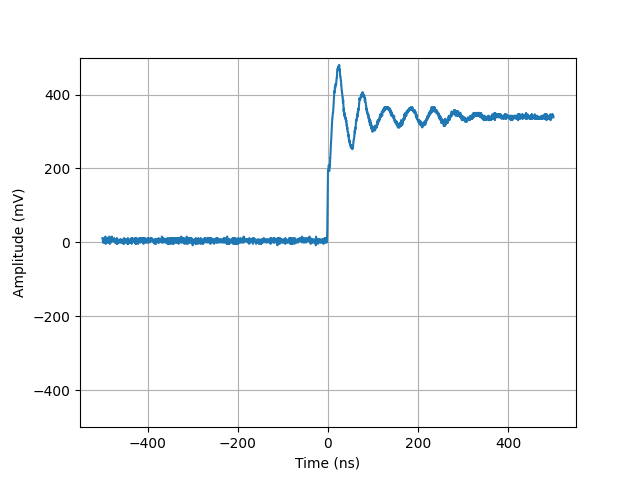
这里卡了挺久的,后面不断的调采集点samples 和 采样间隔 timebase ,才悟出来,这两个东西反相关的。采集间隔小,那么采集点要足够大,才能采集到完整波形;采集间隔大,那采集点就可以不用那么多。
timebase: 采样间隔,用于控制采样率。
timebase 和采集的样本总数samples 共同决定总采集时间窗口:总采集时间 = timebase * samples
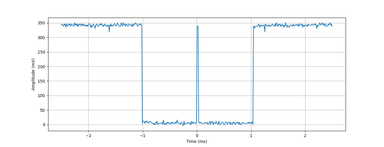
因为采集需求是要大量的traces ,所以这里牺牲采样时长来缓解内存压力,这样采样点就可以少,只是采样时间会变长。
最后采集出来的波长跟示波器捕捉到的一致。
2.3 调整脚本适配分析软件
上面是用 matplotlib 这样直接 show 出来的,跟示波器显示的是一致的。但是业务那边需要采集完再用 inspector 之类的工具去分析,用 inspector 工具打开这个结果,纵坐标是对的,横坐标偏差比较大,单位也不对,故做调整。
后续分析,主要问题是没有配置好横轴采样间隔和偏移量,inspector 会用默认的打开,导致显示不正确。
所以要配置 SCALE_X 和 OFFSET_X 参数,这样 inpsector 会根据这两个参数的值去重建横轴。
SCALE_X:代表X轴每个样本对应的物理量(这里是时间)
OFFSET_X:第一个样本在X轴的起始位置(时间单位)。这样显示的波形横轴就是正确的绝对时间
下面这个脚本是调整后采集多条traces 的,结果保存为 .trs 文件。后续用 inspector 打开 .trs 文件就能正确显示了。
import pypicosdk as psdk
import matplotlib.pyplot as plt
import os
from datetime import datetime
import trsfile
from trsfile import Trace, SampleCoding, TracePadding, Header
import numpy as np

CHANNEL = psdk.CHANNEL.A
VOLTAGE_RANGE = psdk.RANGE.mV500
COUPLING = psdk.COUPLING.DC
TRIGGER_CHANNEL = psdk.CHANNEL.A
TRIGGER_THRESHOLD = 200
TRIGGER_DIRECTION = psdk.TRIGGER_DIR.RISING
# TIMEBASE = 10000000
sample_rate = 9
TOTAL_SAMPLES = 97700
# TOTAL_SAMPLES = 500
TOTAL_CAPTURES = 3


SAVE_DIR = "./captured_traces"
os.makedirs(SAVE_DIR, exist_ok=True)

print("Connecting to PicoScope...")
scope = psdk.psospa()
scope.open_unit()
print("Scope connected.")


try:
    driver_info = scope.get_unit_serial()
    print(f"device info: {driver_info}")
except:
    pass


print("Configuring channel...\n")
scope.set_channel(CHANNEL, enabled=True, coupling=COUPLING, range=VOLTAGE_RANGE)
print("set channel success...\n")


print("Setting trigger...")
scope.set_simple_trigger(
    TRIGGER_CHANNEL,
    threshold=TRIGGER_THRESHOLD,
    direction=TRIGGER_DIRECTION,
    auto_trigger=0
)
print(f"Waiting for trigger on Channel {TRIGGER_CHANNEL} "
      f"({TRIGGER_DIRECTION}, {TRIGGER_THRESHOLD}mV)...")

timebase = scope.sample_rate_to_timebase(sample_rate=sample_rate, unit=psdk.SAMPLE_RATE.MSPS)
channel_buffers, time_axis = scope.run_simple_rapid_block_capture(timebase, TOTAL_SAMPLES, TOTAL_CAPTURES, time_unit="ms")

dt_ms = np.mean(np.diff(time_axis))
dt_s = float(dt_ms*1e-3)

print(f"dt_ms: {dt_ms}, dt_s: {dt_s}")
# print(f"dt_ms: {dt_ms}")

scale_x = dt_s
offset_x = int(time_axis[0]*1e-3)
print(f"scale_x: {scale_x}")
print(f"offset_x: {offset_x}")

all_traces = channel_buffers[psdk.CHANNEL.A]

timestamp = datetime.now().strftime("%Y%m%d_%H%M%S")
filename = f"./captured_traces/traces_{TOTAL_CAPTURES}_{timestamp}.trs"

headers = {
    # Header.DESCRIPTION: 'Encryption traces for side-channel analysis',
    Header.LABEL_X: 's',
    Header.LABEL_Y: 'mV',
    Header.SCALE_X: scale_x,
    Header.OFFSET_X: offset_x
    # Header.SAMPLE_CODING: SampleCoding.FLOAT
}

with trsfile.open(filename, 'w', headers=headers, TracePadding=TracePadding.AUTO) as trs_file:
    for i, trace_data in enumerate(all_traces):
        # metadata = {"tarce_name": f"tarce {i}"}
        trace = Trace(SampleCoding.FLOAT, trace_data, title=f"trace {i}")
        trs_file.append(trace)
        if (i+1) % 200 == 0:
            print(f"Writing trace {i+1}/{len(all_traces)}")
print(f"Saved {len(all_traces)} traces to {filename}")

scope.close_unit()

plt.plot(time_axis, all_traces[-1])
plt.title(f"trace {i}")
plt.xlabel("Time")
plt.ylabel("Amplitude")
plt.grid(True)
plt.show()

print("traces acquisition completed")
2.4 显示额外信息
需求就像挤牙膏一样,擦完一点还有一点。
弄完上面的,又说还差一个显示额外信息,比如密钥、密文什么的。
这个在写入trs 文件的时候,用 Trace() 里面的 parameters 参数传进去。
# 改动的代码
from trsfile.parametermap import  TraceParameterMap
from trsfile.traceparameter import ByteArrayParameter

# trace_param_defs = TraceParameterDefinitionMap()
# trace_param_defs['Data'] = TraceParameterDefinition(bytes, length=0, offset=0)
Keydata = bytes.fromhex('0102030405060708')

with trsfile.open(filename, 'w', headers=headers, TracePadding=TracePadding.AUTO) as trs_file:
    for i, trace_data in enumerate(all_traces):
        # metadata = {"tarce_name": f"tarce {i}"}
        trace_params = TraceParameterMap()
        trace_params['Data'] = ByteArrayParameter(Keydata)
        trace = Trace(SampleCoding.FLOAT, trace_data, title=f"trace {i}", parameters=trace_params)
        trs_file.append(trace)
        if (i+1) % 200 == 0:
            print(f"Writing trace {i+1}/{len(all_traces)}")
print(f"Saved {len(all_traces)} traces to {filename}")
至此,就完成了 PICO示波器的traces 采集。

AtomGit 是由开放原子开源基金会联合 CSDN 等生态伙伴共同推出的新一代开源与人工智能协作平台。平台坚持“开放、中立、公益”的理念,把代码托管、模型共享、数据集托管、智能体开发体验和算力服务整合在一起,为开发者提供从开发、训练到部署的一站式体验。
更多推荐

 9
9 0
0- 0


 已为社区贡献1条内容

所有评论(0)