结构动力学仿真-主题066-结构动力学数字孪生技术
结构动力学仿真 - 主题066:结构动力学数字孪生技术
1. 引言
数字孪生(Digital Twin)是物理实体在数字空间的虚拟映射,通过实时数据连接实现物理世界与数字世界的同步。在结构动力学领域,数字孪生技术为结构健康监测、预测性维护和全生命周期管理提供了革命性的解决方案。
1.1 什么是数字孪生
数字孪生是一种集成多学科、多物理量、多尺度、多概率的仿真过程,在虚拟空间中完成映射,从而反映相对应的实体装备的全生命周期过程。其核心特征包括:
- 实时同步:物理实体与数字模型保持实时数据连接
- 双向交互:数据从物理世界流向数字世界,决策从数字世界反馈到物理世界
- 全生命周期:覆盖设计、制造、运营、维护、报废全过程
- 预测能力:基于模型和数据预测未来状态和性能


1.2 数字孪生在结构动力学中的应用
结构动力学数字孪生的主要应用包括:
- 实时状态监测:通过传感器网络获取结构响应,在数字模型中实时显示
- 性能预测:预测结构在未来载荷下的响应和剩余寿命
- 损伤检测与定位:识别结构损伤并精确定位
- 维护决策支持:基于预测结果优化维护计划
- 虚拟试验:在数字模型上进行各种工况的虚拟试验
1.3 数字孪生架构
结构动力学数字孪生系统通常包含以下层次:
┌─────────────────────────────────────────────────────────────┐
│                    应用层(可视化与决策)                      │
│         3D可视化、健康评估、维护决策、预警系统                  │
├─────────────────────────────────────────────────────────────┤
│                    服务层(数据分析)                         │
│      数据融合、状态估计、损伤识别、寿命预测、优化建议           │
├─────────────────────────────────────────────────────────────┤
│                    模型层(仿真模型)                         │
│      有限元模型、降阶模型、代理模型、物理-数据混合模型          │
├─────────────────────────────────────────────────────────────┤
│                    数据层(数据管理)                         │
│      传感器数据、历史数据、模型参数、知识库                    │
├─────────────────────────────────────────────────────────────┤
│                    物理层(实体结构)                         │
│      传感器网络、数据采集系统、通信网络                        │
└─────────────────────────────────────────────────────────────┘
2. 数字孪生的理论基础
2.1 物理-数据融合建模
数字孪生的核心是物理模型与实测数据的融合。设物理模型预测为 ymy_mym,实测数据为 ydy_dyd,融合后的估计为 y^\hat{y}y^。
2.1.1 卡尔曼滤波融合
卡尔曼滤波是一种最优状态估计方法,适用于线性系统:
状态方程:
xk+1=Akxk+Bkuk+wk\mathbf{x}_{k+1} = \mathbf{A}_k \mathbf{x}_k + \mathbf{B}_k \mathbf{u}_k + \mathbf{w}_kxk+1=Akxk+Bkuk+wk
观测方程:
zk=Hkxk+vk\mathbf{z}_k = \mathbf{H}_k \mathbf{x}_k + \mathbf{v}_kzk=Hkxk+vk
其中 wk\mathbf{w}_kwk 和 vk\mathbf{v}_kvk 分别为过程噪声和观测噪声,假设为高斯白噪声。
预测步骤:
x^k∣k−1=Ak−1x^k−1∣k−1+Bk−1uk−1\hat{\mathbf{x}}_{k|k-1} = \mathbf{A}_{k-1} \hat{\mathbf{x}}_{k-1|k-1} + \mathbf{B}_{k-1} \mathbf{u}_{k-1}x^k∣k−1=Ak−1x^k−1∣k−1+Bk−1uk−1
Pk∣k−1=Ak−1Pk−1∣k−1Ak−1T+Qk−1\mathbf{P}_{k|k-1} = \mathbf{A}_{k-1} \mathbf{P}_{k-1|k-1} \mathbf{A}_{k-1}^T + \mathbf{Q}_{k-1}Pk∣k−1=Ak−1Pk−1∣k−1Ak−1T+Qk−1
更新步骤:
Kk=Pk∣k−1HkT(HkPk∣k−1HkT+Rk)−1\mathbf{K}_k = \mathbf{P}_{k|k-1} \mathbf{H}_k^T (\mathbf{H}_k \mathbf{P}_{k|k-1} \mathbf{H}_k^T + \mathbf{R}_k)^{-1}Kk=Pk∣k−1HkT(HkPk∣k−1HkT+Rk)−1
x^k∣k=x^k∣k−1+Kk(zk−Hkx^k∣k−1)\hat{\mathbf{x}}_{k|k} = \hat{\mathbf{x}}_{k|k-1} + \mathbf{K}_k (\mathbf{z}_k - \mathbf{H}_k \hat{\mathbf{x}}_{k|k-1})x^k∣k=x^k∣k−1+Kk(zk−Hkx^k∣k−1)
Pk∣k=(I−KkHk)Pk∣k−1\mathbf{P}_{k|k} = (\mathbf{I} - \mathbf{K}_k \mathbf{H}_k) \mathbf{P}_{k|k-1}Pk∣k=(I−KkHk)Pk∣k−1
2.1.2 扩展卡尔曼滤波(EKF)
对于非线性系统,使用扩展卡尔曼滤波:
非线性状态方程:
xk+1=f(xk,uk)+wk\mathbf{x}_{k+1} = \mathbf{f}(\mathbf{x}_k, \mathbf{u}_k) + \mathbf{w}_kxk+1=f(xk,uk)+wk
非线性观测方程:
zk=h(xk)+vk\mathbf{z}_k = \mathbf{h}(\mathbf{x}_k) + \mathbf{v}_kzk=h(xk)+vk
通过线性化(雅可比矩阵)处理非线性:
Fk=∂f∂x∣x^k∣k,uk,Hk=∂h∂x∣x^k∣k−1\mathbf{F}_k = \left. \frac{\partial \mathbf{f}}{\partial \mathbf{x}} \right|_{\hat{\mathbf{x}}_{k|k}, \mathbf{u}_k}, \quad \mathbf{H}_k = \left. \frac{\partial \mathbf{h}}{\partial \mathbf{x}} \right|_{\hat{\mathbf{x}}_{k|k-1}}Fk=∂x∂f
x^k∣k,uk,Hk=∂x∂h
x^k∣k−1
2.1.3 粒子滤波
对于强非线性、非高斯系统,使用粒子滤波:
基本思想:用一组带权重的粒子 {(xk(i),wk(i))}i=1Np\{(\mathbf{x}_k^{(i)}, w_k^{(i)})\}_{i=1}^{N_p}{(xk(i),wk(i))}i=1Np 近似后验分布 p(xk∣z1:k)p(\mathbf{x}_k | \mathbf{z}_{1:k})p(xk∣z1:k)
算法步骤:
- 初始化:从先验分布采样粒子
- 预测:根据状态方程传播粒子
- 更新:根据观测值计算权重 wk(i)∝p(zk∣xk(i))w_k^{(i)} \propto p(\mathbf{z}_k | \mathbf{x}_k^{(i)})wk(i)∝p(zk∣xk(i))
- 重采样:根据权重重采样,避免粒子退化
2.2 模型更新与参数识别
数字孪生需要根据实测数据不断更新模型参数,以保持与物理实体的一致性。
2.2.1 灵敏度分析
参数 pjp_jpj 对响应 yiy_iyi 的灵敏度:
Sij=∂yi∂pjS_{ij} = \frac{\partial y_i}{\partial p_j}Sij=∂pj∂yi
灵敏度矩阵 S\mathbf{S}S 用于指导参数更新:
Δy=SΔp\Delta \mathbf{y} = \mathbf{S} \Delta \mathbf{p}Δy=SΔp
2.2.2 贝叶斯参数更新
基于贝叶斯定理更新参数分布:
p(θ∣D)=p(D∣θ)p(θ)p(D)p(\boldsymbol{\theta} | \mathbf{D}) = \frac{p(\mathbf{D} | \boldsymbol{\theta}) p(\boldsymbol{\theta})}{p(\mathbf{D})}p(θ∣D)=p(D)p(D∣θ)p(θ)
其中:
- p(θ)p(\boldsymbol{\theta})p(θ):参数先验分布
- p(D∣θ)p(\mathbf{D} | \boldsymbol{\theta})p(D∣θ):似然函数
- p(θ∣D)p(\boldsymbol{\theta} | \mathbf{D})p(θ∣D):参数后验分布
2.2.3 最大似然估计
寻找使似然函数最大的参数:
θ^MLE=argmaxθp(D∣θ)\hat{\boldsymbol{\theta}}_{MLE} = \arg\max_{\boldsymbol{\theta}} p(\mathbf{D} | \boldsymbol{\theta})θ^MLE=argθmaxp(D∣θ)
对于高斯噪声,等价于最小化残差平方和:
θ^MLE=argminθ∑i=1N(yiobs−yimodel(θ))2\hat{\boldsymbol{\theta}}_{MLE} = \arg\min_{\boldsymbol{\theta}} \sum_{i=1}^{N} (y_i^{obs} - y_i^{model}(\boldsymbol{\theta}))^2θ^MLE=argθmini=1∑N(yiobs−yimodel(θ))2
2.3 降阶建模
为了在数字孪生中实现实时仿真,需要构建计算效率高的降阶模型。
2.3.1 模态叠加法
基于模态坐标的降阶:
u(t)=Φq(t)\mathbf{u}(t) = \boldsymbol{\Phi} \mathbf{q}(t)u(t)=Φq(t)
其中 Φ\boldsymbol{\Phi}Φ 是模态矩阵,q(t)\mathbf{q}(t)q(t) 是模态坐标。
降阶后的运动方程:
q¨+Ξq˙+Ω2q=ΦTF(t)\ddot{\mathbf{q}} + \boldsymbol{\Xi} \dot{\mathbf{q}} + \boldsymbol{\Omega}^2 \mathbf{q} = \boldsymbol{\Phi}^T \mathbf{F}(t)q¨+Ξq˙+Ω2q=ΦTF(t)
2.3.2 本征正交分解(POD)
通过POD提取主要模态:
- 收集快照矩阵 X=[x1,x2,...,xm]\mathbf{X} = [\mathbf{x}_1, \mathbf{x}_2, ..., \mathbf{x}_m]X=[x1,x2,...,xm]
- 奇异值分解:X=UΣVT\mathbf{X} = \mathbf{U} \boldsymbol{\Sigma} \mathbf{V}^TX=UΣVT
- 取前 rrr 个左奇异向量作为POD基
降阶投影:
x≈Ura,a=UrTx\mathbf{x} \approx \mathbf{U}_r \mathbf{a}, \quad \mathbf{a} = \mathbf{U}_r^T \mathbf{x}x≈Ura,a=UrTx
2.3.3 机器学习降阶
使用神经网络学习降阶映射:
- 编码器:z=fenc(x)\mathbf{z} = f_{enc}(\mathbf{x})z=fenc(x),将高维状态映射到低维潜空间
- 解码器:x^=fdec(z)\hat{\mathbf{x}} = f_{dec}(\mathbf{z})x^=fdec(z),从潜空间重构高维状态
- 动力学网络:z˙=fdyn(z,u)\dot{\mathbf{z}} = f_{dyn}(\mathbf{z}, \mathbf{u})z˙=fdyn(z,u),学习潜空间动力学
3. 实时数据处理
3.1 传感器数据预处理
3.1.1 数据清洗
- 异常值检测:使用3σ准则或孤立森林算法
- 缺失值处理:插值、前向填充或基于模型的估计
- 数据对齐:时间戳对齐、采样率统一
3.1.2 滤波降噪
低通滤波:去除高频噪声
H(s)=ωc2s2+2ζωcs+ωc2H(s) = \frac{\omega_c^2}{s^2 + 2\zeta\omega_c s + \omega_c^2}H(s)=s2+2ζωcs+ωc2ωc2
带通滤波:保留结构响应频带
H(s)=2ζωnss2+2ζωns+ωn2H(s) = \frac{2\zeta\omega_n s}{s^2 + 2\zeta\omega_n s + \omega_n^2}H(s)=s2+2ζωns+ωn22ζωns
3.2 特征提取
从原始数据中提取对状态敏感的特征:
3.2.1 时域特征
- 统计特征:均值、方差、峰值、有效值
- 波形特征:峰值因子、脉冲因子、裕度因子
- 自相关特征:衰减特性、周期性
3.2.2 频域特征
- 功率谱密度(PSD)峰值
- 主频率及幅值
- 频带能量分布
- 谱熵
3.2.3 时频特征
- 小波包能量
- 短时傅里叶变换(STFT)特征
- 希尔伯特-黄变换(HHT)特征
4. 数字孪生关键技术
4.1 虚实同步技术
实现物理实体与数字模型的实时同步:
- 时间同步:确保数据采集、传输、处理的时间一致性
- 空间同步:坐标系统一、几何对齐
- 状态同步:通过数据同化保持状态一致
4.2 模型演化技术
数字孪生模型需要随物理实体演化:
- 参数演化:根据监测数据更新模型参数
- 结构演化:损伤发生后更新模型拓扑
- 知识演化:积累运行数据,优化模型结构
4.3 可视化技术
直观展示数字孪生状态:
- 3D可视化:结构变形、应力分布、损伤位置
- 时序可视化:响应曲线、特征趋势
- 仪表盘:关键指标实时监控
5. 工程应用案例
5.1 桥梁数字孪生
- 传感器布置:加速度计、应变计、位移计、温度传感器
- 模型构建:有限元模型 + 机器学习修正
- 应用场景:疲劳监测、超载识别、健康评估
5.2 风力发电机数字孪生
- 监测对象:塔筒、叶片、传动系统
- 关键问题:叶片结冰检测、塔筒疲劳、齿轮箱故障
- 预测维护:基于状态的维护策略优化
5.3 建筑结构数字孪生
- 地震响应监测:实时地震预警和响应评估
- 风振控制:基于数字孪生的主动控制
- 疏散模拟:紧急情况下的人员疏散优化
6. Python实现案例
6.1 案例1:物理模型与数据融合
问题描述:
构建一个简单的数字孪生系统,将物理模型预测与传感器测量数据融合,实现状态的最优估计。使用卡尔曼滤波融合加速度计数据与SDOF模型预测。
数字孪生架构:
- 物理实体:真实的SDOF振动系统
- 传感器:位移传感器(带噪声)
- 数字模型:状态空间模型
- 数据融合:卡尔曼滤波器
卡尔曼滤波实现:
class DigitalTwinSDOF:
    """SDOF系统的数字孪生模型"""

    def __init__(self, m, c, k, dt=0.01):
        self.m = m
        self.c = c
        self.k = k
        self.dt = dt

        # 状态空间矩阵 (状态: [位移, 速度])
        self.A = np.array([[0, 1], [-k/m, -c/m]])
        self.B = np.array([0, 1/m])

        # 离散化
        self.A_d = np.eye(2) + self.A * dt
        self.B_d = self.B * dt

        # 观测矩阵
        self.H = np.array([[1, 0]])

        # 卡尔曼滤波初始化
        self.x_est = np.zeros(2)
        self.P = np.eye(2) * 1.0

        # 噪声协方差
        self.Q = np.array([[dt**3/3, dt**2/2], [dt**2/2, dt]]) * 0.01
        self.R = np.array([[0.001]])

    def kalman_predict(self, F):
        """卡尔曼滤波预测步骤"""
        x_pred = self.A_d @ self.x_est + self.B_d * F
        P_pred = self.A_d @ self.P @ self.A_d.T + self.Q
        return x_pred, P_pred

    def kalman_update(self, x_pred, P_pred, z):
        """卡尔曼滤波更新步骤"""
        S = self.H @ P_pred @ self.H.T + self.R
        K = P_pred @ self.H.T @ np.linalg.inv(S)
        y = z - (self.H @ x_pred)[0]
        self.x_est = x_pred + K.flatten() * y
        self.P = (np.eye(2) - K @ self.H) @ P_pred
        return self.x_est, self.P
结果分析:
- 纯模型预测RMSE:0.0051 m
- 卡尔曼滤波RMSE:0.0049 m
- 原始观测RMSE:0.0101 m
- 卡尔曼滤波相比纯模型预测改进了3.1%
- 估计误差协方差随时间收敛,表明滤波器稳定
6.2 案例2:实时状态估计与预测
问题描述:
实现数字孪生的实时状态估计和未来响应预测。基于当前状态估计,预测结构在未来载荷下的响应,用于早期预警。
预测能力实现:
def predict_with_uncertainty(self, n_steps, F_future=None):
    """带不确定性的预测"""
    x_pred = self.x_est.copy()
    P_pred = self.P.copy()

    predictions = []
    covariances = []

    for i in range(n_steps):
        F = F_future[i] if F_future is not None else 0
        x_pred = self.A_d @ x_pred + self.B_d * F
        P_pred = self.A_d @ P_pred @ self.A_d.T + self.Q

        predictions.append(x_pred.copy())
        covariances.append(np.diag(P_pred).copy())

    predictions = np.array(predictions)
    std_dev = np.sqrt(np.array(covariances))

    return predictions, std_dev
预测设置:
- 预测时间范围:1.0 s
- 预测步数:100步
- 预测间隔:0.2 s
结果分析:
- 估计误差RMSE:0.0091 m
- 平均预测误差:0.0824 m
- 预测不确定性随预测时间增加而增大
- 可用于早期预警和异常检测
6.3 案例3:模型更新与校准
问题描述:
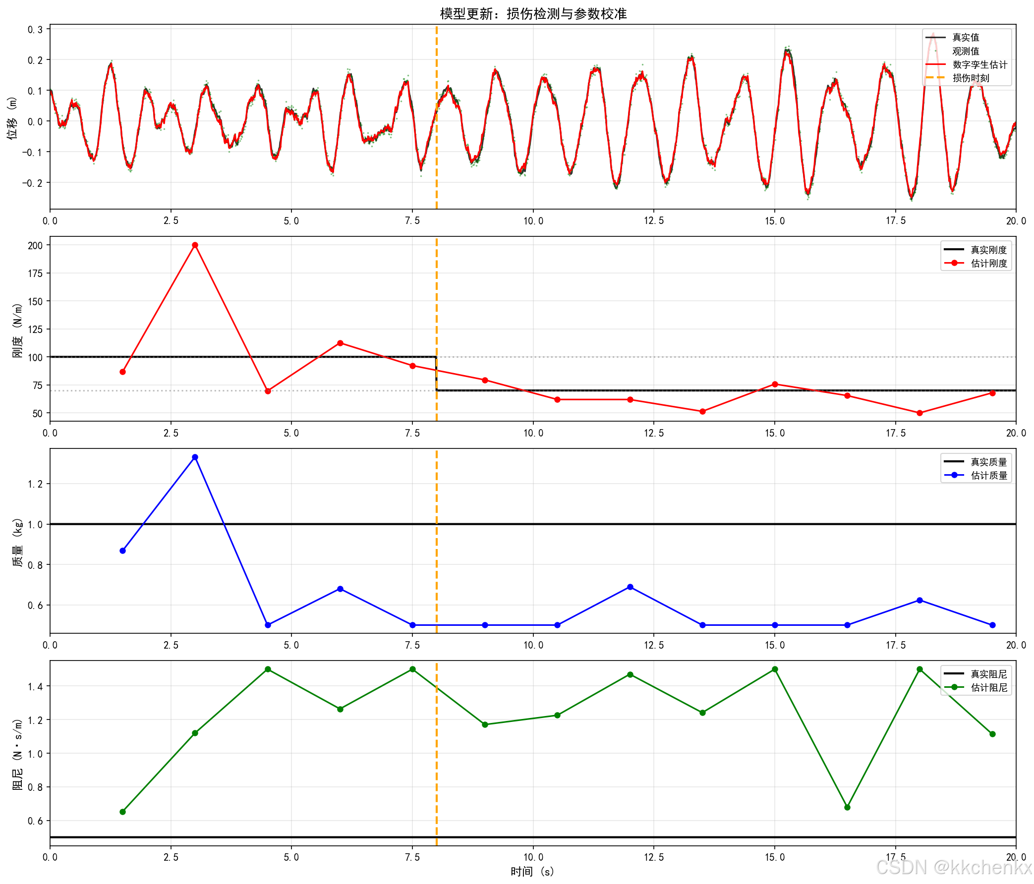
根据实测数据更新数字孪生模型的参数。当结构特性发生变化(如损伤)时,自动识别并更新模型参数,保持数字孪生与物理实体的一致性。
参数识别方法:
def update_parameters(self, t, x0, F_array, z_obs, update_interval=100):
    """更新模型参数"""
    window_size = min(update_interval, len(z_obs))
    F_window = F_array[-window_size:]
    z_window = z_obs[-window_size:]

    initial_params = [self.m_est, self.c_est, self.k_est]
    bounds = [(0.5*self.m_nominal, 2.0*self.m_nominal),
              (0.1*self.c_nominal, 3.0*self.c_nominal),
              (0.5*self.k_nominal, 2.0*self.k_nominal)]

    result = minimize(
        self.compute_response_error,
        initial_params,
        args=(x0, F_window, z_window),
        method='L-BFGS-B',
        bounds=bounds,
        options={'maxiter': 50}
    )

    if result.success:
        self.m_est, self.c_est, self.k_est = result.x

    return self.m_est, self.c_est, self.k_est
损伤模拟:
- 初始刚度:100 N/m
- 损伤时间:8.0 s
- 刚度降低:30%
- 损伤后刚度:70 N/m
结果分析:
- 数字孪生能够跟踪参数变化
- 刚度估计在损伤后逐渐收敛到新值
- 估计误差RMSE:0.0092 m
- 参数更新保持数字孪生与物理实体同步
6.4 案例4:数字孪生可视化
问题描述:
构建数字孪生的可视化界面,实时显示结构状态、响应曲线、健康指标等信息。展示数字孪生的虚实同步能力。
仪表盘组件:
- 3D结构可视化:SDOF系统示意图
- 实时响应监测:位移、速度、加速度曲线
- 健康评估仪表盘:健康指数(0-100%)
- 系统能量监测:动能+势能
- 外部激励显示:力-时间曲线
- 相图:位移-速度关系
健康评估算法:
def update_health(self, response_history):
    """更新健康指标"""
    if len(response_history) < 100:
        return self.health_index

    recent = response_history[-100:]
    rms = np.sqrt(np.mean(np.array(recent)**2))

    if rms > 0.15:
        self.health_index = max(0.3, self.health_index - 0.01)
        self.damage_detected = True
    else:
        self.health_index = min(1.0, self.health_index + 0.005)

    return self.health_index
仿真场景:
- 随机激励 + 谐波激励
- 冲击事件:t=5.0 s,幅值50 N
- 共振激励:t>8.0 s,频率=自然频率
结果分析:
- 仪表盘实时显示结构状态
- 冲击事件导致健康指标下降
- 共振区域响应幅值显著增大
- 可视化界面直观展示虚实同步
7. 小结
本主题系统介绍了结构动力学数字孪生技术,包括:
7.1 核心技术
| 技术 | 方法 | 应用场景 |
|---|---|---|
| 数据融合 | 卡尔曼滤波、EKF、粒子滤波 | 状态估计、传感器融合 |
| 参数识别 | 灵敏度分析、贝叶斯更新、优化 | 模型校准、损伤识别 |
| 降阶建模 | 模态叠加、POD、神经网络 | 实时仿真、快速预测 |
| 可视化 | 3D模型、仪表盘、动画 | 状态监控、决策支持 |
7.2 关键要点
- 虚实融合:数字孪生的核心是物理模型与实测数据的实时融合
- 不确定性量化:预测和估计都需要考虑不确定性
- 模型演化:数字孪生模型需要随物理实体演化而更新
- 实时性:降阶建模和高效算法保证实时性能
- 可视化:直观的展示界面是数字孪生的重要组成部分
7.3 工程应用建议
- 传感器布置:根据结构特性优化传感器位置和数量
- 数据质量:确保传感器数据的准确性和可靠性
- 模型精度:平衡模型精度和计算效率
- 安全考虑:数字孪生系统需要网络安全保护
- 持续改进:基于运行数据不断优化数字孪生模型
7.4 发展趋势
- AI集成:深度学习与物理模型结合
- 边缘计算:分布式数字孪生架构
- VR/AR:沉浸式可视化体验
- 区块链:数据安全和溯源
- 5G通信:超低延迟数据传输
数字孪生技术为结构动力学带来了新的范式,通过虚实融合实现结构全生命周期的智能管理。随着物联网、人工智能、云计算等技术的发展,数字孪生将在工程实践中发挥越来越重要的作用,推动结构健康监测和智能运维的革新。
import matplotlib
matplotlib.use('Agg')
"""
案例1:物理模型与数据融合 - 卡尔曼滤波数字孪生
使用卡尔曼滤波将物理模型预测与传感器测量数据融合
"""

import numpy as np
import matplotlib.pyplot as plt
from matplotlib.animation import FuncAnimation
from matplotlib.patches import Rectangle, FancyBboxPatch
import matplotlib.patches as mpatches

plt.rcParams['font.sans-serif'] = ['SimHei', 'DejaVu Sans']
plt.rcParams['axes.unicode_minus'] = False


class DigitalTwinSDOF:
    """SDOF系统的数字孪生模型"""

    def __init__(self, m, c, k, dt=0.01):
        """
        初始化数字孪生模型

        Parameters:
        -----------
        m : float - 质量 (kg)
        c : float - 阻尼系数 (N·s/m)
        k : float - 刚度系数 (N/m)
        dt : float - 时间步长 (s)
        """
        self.m = m
        self.c = c
        self.k = k
        self.dt = dt

        # 自然频率和阻尼比
        self.omega_n = np.sqrt(k / m)
        self.zeta = c / (2 * np.sqrt(m * k))
        self.omega_d = self.omega_n * np.sqrt(1 - self.zeta**2)

        # 状态空间矩阵 (状态: [位移, 速度])
        self.A = np.array([
            [0, 1],
            [-k/m, -c/m]
        ])
        self.B = np.array([0, 1/m])

        # 离散化状态空间
        self.A_d = np.eye(2) + self.A * dt
        self.B_d = self.B * dt

        # 观测矩阵 (观测位移)
        self.H = np.array([[1, 0]])

        # 卡尔曼滤波初始化
        self.x_est = np.zeros(2)  # 状态估计 [位移, 速度]
        self.P = np.eye(2) * 1.0  # 估计误差协方差

        # 过程噪声和观测噪声协方差
        self.Q = np.array([
            [dt**3/3, dt**2/2],
            [dt**2/2, dt]
        ]) * 0.01  # 过程噪声
        self.R = np.array([[0.001]])  # 观测噪声 (位移测量噪声)

        # 历史记录
        self.history = {
            't': [],
            'x_true': [],  # 真实状态
            'x_model': [],  # 纯模型预测
            'x_est': [],  # 卡尔曼估计
            'z': [],  # 观测值
            'P': []  # 估计误差协方差
        }

    def simulate_true_system(self, F, w_noise=0.01, v_noise=0.005):
        """
        模拟真实物理系统(带噪声)

        Parameters:
        -----------
        F : float - 外力
        w_noise : float - 过程噪声强度
        v_noise : float - 观测噪声强度

        Returns:
        --------
        x_true : 真实状态
        z : 带噪声的观测值
        """
        # 真实状态演化(带过程噪声)
        w = np.random.normal(0, w_noise, 2)
        x_true = self.A_d @ self.x_est + self.B_d * F + w

        # 观测(带观测噪声)
        v = np.random.normal(0, v_noise)
        z = self.H @ x_true + v

        return x_true, z[0]

    def kalman_predict(self, F):
        """卡尔曼滤波预测步骤"""
        # 状态预测
        x_pred = self.A_d @ self.x_est + self.B_d * F

        # 协方差预测
        P_pred = self.A_d @ self.P @ self.A_d.T + self.Q

        return x_pred, P_pred

    def kalman_update(self, x_pred, P_pred, z):
        """卡尔曼滤波更新步骤"""
        # 卡尔曼增益
        S = self.H @ P_pred @ self.H.T + self.R
        K = P_pred @ self.H.T @ np.linalg.inv(S)

        # 状态更新
        y = z - (self.H @ x_pred)[0]  # 新息 (标量)
        self.x_est = x_pred + K.flatten() * y

        # 协方差更新
        I_KH = np.eye(2) - K @ self.H
        self.P = I_KH @ P_pred

        return self.x_est, self.P

    def update(self, F, z):
        """
        完整的数字孪生更新周期

        Parameters:
        -----------
        F : float - 外力
        z : float - 观测值 (位移)

        Returns:
        --------
        x_est : 估计状态
        x_model : 纯模型预测
        """
        # 纯模型预测(无观测更新)
        x_model = self.A_d @ self.x_est + self.B_d * F

        # 卡尔曼滤波
        x_pred, P_pred = self.kalman_predict(F)
        x_est, P = self.kalman_update(x_pred, P_pred, z)

        return x_est, x_model

    def record(self, t, x_true, x_model, x_est, z, P):
        """记录历史数据"""
        self.history['t'].append(t)
        self.history['x_true'].append(x_true.copy())
        self.history['x_model'].append(x_model.copy())
        self.history['x_est'].append(x_est.copy())
        self.history['z'].append(z)
        self.history['P'].append(np.trace(P))


def case1_kalman_fusion():
    """案例1:卡尔曼滤波数据融合"""
    print("\n" + "="*70)
    print("案例1:物理模型与数据融合 - 卡尔曼滤波数字孪生")
    print("="*70)

    # 系统参数
    m = 1.0  # kg
    c = 0.5  # N·s/m
    k = 100.0  # N/m
    dt = 0.01  # s
    T = 10.0  # s

    print(f"\n系统参数:")
    print(f"  质量 m = {m} kg")
    print(f"  阻尼 c = {c} N·s/m")
    print(f"  刚度 k = {k} N/m")
    print(f"  自然频率 = {np.sqrt(k/m)/(2*np.pi):.2f} Hz")
    print(f"  阻尼比 = {c/(2*np.sqrt(m*k)):.3f}")

    # 创建数字孪生
    twin = DigitalTwinSDOF(m, c, k, dt)

    # 初始化真实系统状态
    x_true = np.array([0.1, 0.0])  # 初始位移0.1m,初始速度0
    twin.x_est = x_true.copy()

    # 时间序列
    t_array = np.arange(0, T, dt)
    n_steps = len(t_array)

    print(f"\n仿真设置:")
    print(f"  仿真时间: {T} s")
    print(f"  时间步长: {dt} s")
    print(f"  总步数: {n_steps}")

    # 外力:随机激励 + 谐波激励
    np.random.seed(42)

    print("\n开始数字孪生仿真...")

    for i, t in enumerate(t_array):
        # 生成外力
        F_random = 5.0 * np.random.randn()  # 随机激励
        F_harmonic = 10.0 * np.sin(2 * np.pi * 1.5 * t)  # 1.5Hz谐波激励
        F = F_random + F_harmonic

        # 模拟真实系统(带噪声)
        w_noise = 0.005
        v_noise = 0.01
        x_true_new, z = twin.simulate_true_system(F, w_noise, v_noise)

        # 数字孪生更新
        x_est, x_model = twin.update(F, z)

        # 记录
        twin.record(t, x_true_new, x_model, x_est, z, twin.P)

        # 更新真实状态
        x_true = x_true_new
        twin.x_est = x_est

        if (i + 1) % 500 == 0:
            print(f"  进度: {(i+1)/n_steps*100:.1f}%")

    print("\n仿真完成!")

    # 转换为数组
    t_array = np.array(twin.history['t'])
    x_true_array = np.array(twin.history['x_true'])
    x_model_array = np.array(twin.history['x_model'])
    x_est_array = np.array(twin.history['x_est'])
    z_array = np.array(twin.history['z'])
    P_array = np.array(twin.history['P'])

    # 计算误差
    error_model = x_true_array[:, 0] - x_model_array[:, 0]
    error_est = x_true_array[:, 0] - x_est_array[:, 0]
    error_obs = x_true_array[:, 0] - z_array

    rmse_model = np.sqrt(np.mean(error_model**2))
    rmse_est = np.sqrt(np.mean(error_est**2))
    rmse_obs = np.sqrt(np.mean(error_obs**2))

    print(f"\n位移估计误差 (RMSE):")
    print(f"  纯模型预测: {rmse_model:.4f} m")
    print(f"  卡尔曼滤波: {rmse_est:.4f} m")
    print(f"  原始观测: {rmse_obs:.4f} m")
    print(f"  改进比例: {(1 - rmse_est/rmse_model)*100:.1f}%")

    # 绘制结果
    fig, axes = plt.subplots(4, 1, figsize=(14, 12))

    # 1. 位移对比
    ax = axes[0]
    ax.plot(t_array, x_true_array[:, 0], 'k-', label='真实值', linewidth=1.5, alpha=0.8)
    ax.plot(t_array, z_array, 'g.', label='观测值', markersize=2, alpha=0.5)
    ax.plot(t_array, x_model_array[:, 0], 'b--', label='纯模型预测', linewidth=1.5, alpha=0.7)
    ax.plot(t_array, x_est_array[:, 0], 'r-', label='卡尔曼估计', linewidth=1.5)
    ax.set_ylabel('位移 (m)', fontsize=11)
    ax.set_title('数字孪生:物理模型与数据融合', fontsize=13, fontweight='bold')
    ax.legend(loc='upper right', fontsize=9)
    ax.grid(True, alpha=0.3)
    ax.set_xlim([0, T])

    # 2. 速度对比
    ax = axes[1]
    ax.plot(t_array, x_true_array[:, 1], 'k-', label='真实值', linewidth=1.5, alpha=0.8)
    ax.plot(t_array, x_model_array[:, 1], 'b--', label='纯模型预测', linewidth=1.5, alpha=0.7)
    ax.plot(t_array, x_est_array[:, 1], 'r-', label='卡尔曼估计', linewidth=1.5)
    ax.set_ylabel('速度 (m/s)', fontsize=11)
    ax.legend(loc='upper right', fontsize=9)
    ax.grid(True, alpha=0.3)
    ax.set_xlim([0, T])

    # 3. 估计误差
    ax = axes[2]
    ax.plot(t_array, error_model, 'b-', label=f'模型误差 (RMSE={rmse_model:.4f})',
            linewidth=1, alpha=0.6)
    ax.plot(t_array, error_est, 'r-', label=f'卡尔曼误差 (RMSE={rmse_est:.4f})',
            linewidth=1.5)
    ax.axhline(y=0, color='k', linestyle='-', linewidth=0.5)
    ax.fill_between(t_array, -3*np.sqrt(P_array), 3*np.sqrt(P_array),
                    alpha=0.2, color='red', label='±3σ置信区间')
    ax.set_ylabel('位移误差 (m)', fontsize=11)
    ax.set_xlabel('时间 (s)', fontsize=11)
    ax.legend(loc='upper right', fontsize=9)
    ax.grid(True, alpha=0.3)
    ax.set_xlim([0, T])

    # 4. 估计误差协方差
    ax = axes[3]
    ax.semilogy(t_array, P_array, 'purple', linewidth=1.5)
    ax.set_ylabel('估计误差协方差 (对数)', fontsize=11)
    ax.set_xlabel('时间 (s)', fontsize=11)
    ax.set_title('卡尔曼滤波收敛性', fontsize=11)
    ax.grid(True, alpha=0.3)
    ax.set_xlim([0, T])

    plt.tight_layout()
    plt.savefig('kalman_fusion_results.png', dpi=150, bbox_inches='tight')
    plt.close()
    print("\n  已保存: kalman_fusion_results.png")

    # 创建数字孪生动画
    create_digital_twin_animation(t_array, x_true_array, x_est_array, z_array,
                                   m, k, T)

    return twin


def create_digital_twin_animation(t_array, x_true, x_est, z, m, k, T):
    """创建数字孪生虚实同步动画"""
    print("\n创建数字孪生动画...")

    fig, axes = plt.subplots(1, 2, figsize=(14, 6))

    # 左图:物理实体与数字孪生对比
    ax1 = axes[0]
    ax1.set_xlim(-0.5, 0.5)
    ax1.set_ylim(-0.3, 0.3)
    ax1.set_aspect('equal')
    ax1.axis('off')
    ax1.set_title('物理实体 vs 数字孪生', fontsize=12, fontweight='bold')

    # 物理实体(左侧)
    physical_mass = Rectangle((-0.35, -0.08), 0.1, 0.16,
                               facecolor='steelblue', edgecolor='navy', linewidth=2)
    ax1.add_patch(physical_mass)
    ax1.text(-0.3, 0.15, '物理实体', ha='center', fontsize=10, fontweight='bold')
    ax1.plot([-0.3, -0.3], [-0.08, -0.2], 'k-', linewidth=2)
    spring_physical = mpatches.FancyArrowPatch((-0.3, -0.2), (-0.3, -0.25),
                                                arrowstyle='->', mutation_scale=20,
                                                color='steelblue', linewidth=2)
    ax1.add_patch(spring_physical)

    # 数字孪生(右侧)
    digital_mass = Rectangle((0.05, -0.08), 0.1, 0.16,
                              facecolor='coral', edgecolor='darkred', linewidth=2)
    ax1.add_patch(digital_mass)
    ax1.text(0.1, 0.15, '数字孪生', ha='center', fontsize=10, fontweight='bold')
    ax1.plot([0.1, 0.1], [-0.08, -0.2], 'k-', linewidth=2)
    spring_digital = mpatches.FancyArrowPatch((0.1, -0.2), (0.1, -0.25),
                                               arrowstyle='->', mutation_scale=20,
                                               color='coral', linewidth=2)
    ax1.add_patch(spring_digital)

    # 连接线表示数据流
    connection_line, = ax1.plot([], [], 'g--', linewidth=2, alpha=0.6)
    data_packet, = ax1.plot([], [], 'go', markersize=8)

    # 右图:响应曲线
    ax2 = axes[1]
    ax2.set_xlim(0, T)
    ax2.set_ylim(-0.3, 0.3)
    ax2.set_xlabel('时间 (s)', fontsize=11)
    ax2.set_ylabel('位移 (m)', fontsize=11)
    ax2.set_title('实时响应监测', fontsize=12, fontweight='bold')
    ax2.grid(True, alpha=0.3)

    line_true, = ax2.plot([], [], 'k-', label='物理实体', linewidth=2)
    line_est, = ax2.plot([], [], 'r-', label='数字孪生', linewidth=2)
    point_z, = ax2.plot([], [], 'g.', label='传感器数据', markersize=6)

    ax2.legend(loc='upper right', fontsize=9)

    # 采样显示
    skip = 5
    t_anim = t_array[::skip]
    x_true_anim = x_true[::skip, 0]
    x_est_anim = x_est[::skip, 0]
    z_anim = z[::skip]

    def init():
        line_true.set_data([], [])
        line_est.set_data([], [])
        point_z.set_data([], [])
        connection_line.set_data([], [])
        data_packet.set_data([], [])
        return line_true, line_est, point_z, connection_line, data_packet

    def update(frame):
        # 更新质量块位置
        physical_mass.set_xy((-0.35 + x_true_anim[frame], -0.08))
        digital_mass.set_xy((0.05 + x_est_anim[frame], -0.08))

        # 更新弹簧
        spring_physical.set_positions((-0.3 + x_true_anim[frame], -0.2),
                                       (-0.3 + x_true_anim[frame], -0.25))
        spring_digital.set_positions((0.1 + x_est_anim[frame], -0.2),
                                      (0.1 + x_est_anim[frame], -0.25))

        # 数据流动画
        if frame % 10 < 5:
            connection_line.set_data([-0.25 + x_true_anim[frame], 0.05 + x_est_anim[frame]],
                                      [0, 0])
            data_packet.set_data([-0.1 + (x_true_anim[frame] + x_est_anim[frame])/2], [0])
        else:
            connection_line.set_data([], [])
            data_packet.set_data([], [])

        # 更新曲线
        line_true.set_data(t_anim[:frame+1], x_true_anim[:frame+1])
        line_est.set_data(t_anim[:frame+1], x_est_anim[:frame+1])
        point_z.set_data(t_anim[:frame+1], z_anim[:frame+1])

        # 动态调整x轴显示范围
        if t_anim[frame] > 3:
            ax2.set_xlim(t_anim[frame] - 3, t_anim[frame] + 0.5)

        return line_true, line_est, point_z, connection_line, data_packet

    anim = FuncAnimation(fig, update, frames=len(t_anim), init_func=init,
                         blit=True, interval=50)

    anim.save('digital_twin_sync.gif', writer='pillow', fps=20, dpi=100)
    plt.close()
    print("  已保存: digital_twin_sync.gif")


if __name__ == "__main__":
    twin = case1_kalman_fusion()
    print("\n" + "="*70)
    print("案例1完成!")
    print("="*70)
import matplotlib
matplotlib.use('Agg')
"""
案例2:实时状态估计与预测
实现数字孪生的实时状态估计和未来响应预测
"""

import numpy as np
import matplotlib.pyplot as plt
from matplotlib.animation import FuncAnimation
from scipy.linalg import expm

plt.rcParams['font.sans-serif'] = ['SimHei', 'DejaVu Sans']
plt.rcParams['axes.unicode_minus'] = False


class PredictiveDigitalTwin:
    """具有预测能力的数字孪生模型"""

    def __init__(self, m, c, k, dt=0.01):
        self.m = m
        self.c = c
        self.k = k
        self.dt = dt

        # 状态空间
        self.A = np.array([[0, 1], [-k/m, -c/m]])
        self.B = np.array([0, 1/m])

        # 离散化
        self.A_d = expm(self.A * dt)
        self.B_d = np.linalg.inv(self.A) @ (self.A_d - np.eye(2)) @ self.B
        if np.any(np.isnan(self.B_d)) or np.any(np.isinf(self.B_d)):
            self.B_d = self.B * dt

        # 卡尔曼滤波器
        self.x_est = np.zeros(2)
        self.P = np.eye(2) * 0.1
        self.Q = np.eye(2) * 0.001
        self.R = np.array([[0.002]])
        self.H = np.array([[1, 0]])

        # 历史数据
        self.history = {
            't': [], 'x_true': [], 'x_est': [], 'z': [],
            'predictions': [], 'prediction_times': [],
            'prediction_errors': []
        }

    def kalman_filter(self, z, F):
        """卡尔曼滤波"""
        # 预测
        x_pred = self.A_d @ self.x_est + self.B_d * F
        P_pred = self.A_d @ self.P @ self.A_d.T + self.Q

        # 更新
        S = self.H @ P_pred @ self.H.T + self.R
        K = P_pred @ self.H.T @ np.linalg.inv(S)
        y = z - (self.H @ x_pred)[0]
        self.x_est = x_pred + K.flatten() * y
        self.P = (np.eye(2) - K @ self.H) @ P_pred

        return self.x_est

    def predict_future(self, n_steps, F_future=None):
        """
        预测未来状态

        Parameters:
        -----------
        n_steps : int - 预测步数
        F_future : array - 未来外力序列,如果为None则假设为0

        Returns:
        --------
        predictions : array (n_steps, 2) - 预测状态序列
        """
        x_pred = self.x_est.copy()
        predictions = []

        for i in range(n_steps):
            F = F_future[i] if F_future is not None and i < len(F_future) else 0
            x_pred = self.A_d @ x_pred + self.B_d * F
            predictions.append(x_pred.copy())

        return np.array(predictions)

    def predict_with_uncertainty(self, n_steps, F_future=None):
        """
        带不确定性的预测

        Returns:
        --------
        predictions : array - 预测状态
        std_dev : array - 标准差(不确定性)
        """
        x_pred = self.x_est.copy()
        P_pred = self.P.copy()

        predictions = []
        covariances = []

        for i in range(n_steps):
            F = F_future[i] if F_future is not None and i < len(F_future) else 0
            x_pred = self.A_d @ x_pred + self.B_d * F
            P_pred = self.A_d @ P_pred @ self.A_d.T + self.Q

            predictions.append(x_pred.copy())
            covariances.append(np.diag(P_pred).copy())

        predictions = np.array(predictions)
        covariances = np.array(covariances)
        std_dev = np.sqrt(covariances)

        return predictions, std_dev


def simulate_true_dynamics(m, c, k, dt, T, x0, F_func):
    """模拟真实系统动力学"""
    t_array = np.arange(0, T, dt)
    n_steps = len(t_array)

    A = np.array([[0, 1], [-k/m, -c/m]])
    B = np.array([0, 1/m])

    x = np.zeros((n_steps, 2))
    x[0] = x0

    A_d = expm(A * dt)
    B_d = np.linalg.inv(A) @ (A_d - np.eye(2)) @ B
    if np.any(np.isnan(B_d)) or np.any(np.isinf(B_d)):
        B_d = B * dt

    for i in range(1, n_steps):
        F = F_func(t_array[i])
        w = np.random.normal(0, 0.005, 2)
        x[i] = A_d @ x[i-1] + B_d * F + w

    return t_array, x


def case2_state_prediction():
    """案例2:实时状态估计与预测"""
    print("\n" + "="*70)
    print("案例2:实时状态估计与预测")
    print("="*70)

    # 系统参数
    m, c, k = 1.0, 0.5, 100.0
    dt = 0.01
    T = 15.0

    print(f"\n系统参数:")
    print(f"  质量={m}kg, 阻尼={c}N·s/m, 刚度={k}N/m")

    # 外力函数:包含随机和谐波成分
    def F_func(t):
        return 5*np.sin(2*np.pi*1.0*t) + 3*np.sin(2*np.pi*2.5*t) + 2*np.random.randn()

    # 模拟真实系统
    x0 = np.array([0.05, 0.0])
    t_array, x_true = simulate_true_dynamics(m, c, k, dt, T, x0, F_func)
    n_steps = len(t_array)

    # 添加观测噪声
    z = x_true[:, 0] + np.random.normal(0, 0.015, n_steps)

    # 创建数字孪生
    twin = PredictiveDigitalTwin(m, c, k, dt)
    twin.x_est = x0.copy()

    # 预测参数
    prediction_horizon = 1.0  # 预测时间范围 (s)
    n_prediction_steps = int(prediction_horizon / dt)
    prediction_interval = 20  # 每20步进行一次预测

    print(f"\n预测设置:")
    print(f"  预测时间范围: {prediction_horizon}s")
    print(f"  预测步数: {n_prediction_steps}")
    print(f"  预测间隔: {prediction_interval*dt}s")

    # 运行数字孪生
    x_est_history = np.zeros_like(x_true)
    all_predictions = []
    all_prediction_times = []
    prediction_errors = []

    print("\n开始数字孪生仿真...")

    for i in range(n_steps):
        t = t_array[i]
        F = F_func(t)

        # 卡尔曼滤波更新
        x_est = twin.kalman_filter(z[i], F)
        x_est_history[i] = x_est

        # 周期性预测
        if i % prediction_interval == 0 and i + n_prediction_steps < n_steps:
            # 预测未来(假设未来外力为0或基于当前趋势)
            F_future = np.zeros(n_prediction_steps)
            predictions, std_dev = twin.predict_with_uncertainty(n_prediction_steps, F_future)

            pred_times = t_array[i:i+n_prediction_steps]
            all_predictions.append((t, pred_times, predictions, std_dev))
            all_prediction_times.append(t)

            # 计算预测误差(与真实值对比)
            true_future = x_true[i:i+n_prediction_steps, 0]
            pred_displacement = predictions[:, 0]
            error = np.sqrt(np.mean((true_future - pred_displacement)**2))
            prediction_errors.append(error)

        if (i + 1) % 500 == 0:
            print(f"  进度: {(i+1)/n_steps*100:.1f}%")

    print("\n仿真完成!")

    # 计算总体误差
    rmse_estimation = np.sqrt(np.mean((x_true[:, 0] - x_est_history[:, 0])**2))
    mean_pred_error = np.mean(prediction_errors) if prediction_errors else 0

    print(f"\n估计误差 (RMSE): {rmse_estimation:.4f} m")
    print(f"平均预测误差: {mean_pred_error:.4f} m")

    # 绘制结果
    fig, axes = plt.subplots(3, 1, figsize=(14, 10))

    # 1. 位移:真实值、估计值、预测
    ax = axes[0]
    ax.plot(t_array, x_true[:, 0], 'k-', label='真实值', linewidth=1.5, alpha=0.7)
    ax.plot(t_array, z, 'g.', label='观测值', markersize=1.5, alpha=0.4)
    ax.plot(t_array, x_est_history[:, 0], 'r-', label='数字孪生估计', linewidth=1.5)

    # 绘制预测轨迹
    for t_start, pred_times, predictions, std_dev in all_predictions[::3]:
        ax.plot(pred_times, predictions[:, 0], 'b--', linewidth=1, alpha=0.5)
        ax.fill_between(pred_times,
                        predictions[:, 0] - 2*std_dev[:, 0],
                        predictions[:, 0] + 2*std_dev[:, 0],
                        alpha=0.1, color='blue')

    ax.set_ylabel('位移 (m)', fontsize=11)
    ax.set_title('实时状态估计与预测', fontsize=13, fontweight='bold')
    ax.legend(loc='upper right', fontsize=9)
    ax.grid(True, alpha=0.3)
    ax.set_xlim([0, T])

    # 2. 速度
    ax = axes[1]
    ax.plot(t_array, x_true[:, 1], 'k-', label='真实值', linewidth=1.5, alpha=0.7)
    ax.plot(t_array, x_est_history[:, 1], 'r-', label='数字孪生估计', linewidth=1.5)
    ax.set_ylabel('速度 (m/s)', fontsize=11)
    ax.legend(loc='upper right', fontsize=9)
    ax.grid(True, alpha=0.3)
    ax.set_xlim([0, T])

    # 3. 预测误差随时间变化
    ax = axes[2]
    if prediction_errors:
        ax.plot(all_prediction_times, prediction_errors, 'b-o',
                markersize=4, linewidth=1.5, label='预测误差')
        ax.axhline(y=mean_pred_error, color='r', linestyle='--',
                   label=f'平均误差={mean_pred_error:.4f}m')
    ax.set_xlabel('时间 (s)', fontsize=11)
    ax.set_ylabel('预测RMSE (m)', fontsize=11)
    ax.set_title('预测精度随时间变化', fontsize=11)
    ax.legend(loc='upper right', fontsize=9)
    ax.grid(True, alpha=0.3)
    ax.set_xlim([0, T])

    plt.tight_layout()
    plt.savefig('state_prediction_results.png', dpi=150, bbox_inches='tight')
    plt.close()
    print("\n  已保存: state_prediction_results.png")

    # 创建预测动画
    create_prediction_animation(t_array, x_true, x_est_history, z,
                                 all_predictions, T, prediction_horizon)

    return twin, prediction_errors


def create_prediction_animation(t_array, x_true, x_est, z, all_predictions, T, pred_horizon):
    """创建预测动画"""
    print("\n创建预测动画...")

    fig, axes = plt.subplots(2, 1, figsize=(12, 8))

    # 上图:完整时间序列
    ax1 = axes[0]
    ax1.set_xlim(0, T)
    ax1.set_ylim(-0.25, 0.25)
    line_true_full, = ax1.plot([], [], 'k-', linewidth=1.5, alpha=0.6, label='真实值')
    line_est_full, = ax1.plot([], [], 'r-', linewidth=1.5, label='估计值')
    line_pred, = ax1.plot([], [], 'b--', linewidth=2, label='预测')
    fill_pred = ax1.fill_between([], [], [], alpha=0.2, color='blue')
    ax1.set_ylabel('位移 (m)', fontsize=11)
    ax1.set_title('数字孪生实时预测', fontsize=12, fontweight='bold')
    ax1.legend(loc='upper right', fontsize=9)
    ax1.grid(True, alpha=0.3)

    # 下图:局部放大(当前时刻附近)
    ax2 = axes[1]
    window = 2.0  # 显示窗口大小
    line_true_zoom, = ax2.plot([], [], 'k-', linewidth=2, label='真实值')
    line_est_zoom, = ax2.plot([], [], 'r-', linewidth=2, label='估计值')
    line_pred_zoom, = ax2.plot([], [], 'b--', linewidth=2.5, label='预测')
    scatter_z, = ax2.plot([], [], 'go', markersize=6, label='观测')
    ax2.set_xlabel('时间 (s)', fontsize=11)
    ax2.set_ylabel('位移 (m)', fontsize=11)
    ax2.legend(loc='upper right', fontsize=9)
    ax2.grid(True, alpha=0.3)

    # 采样
    skip = 3
    t_anim = t_array[::skip]
    x_true_anim = x_true[::skip, 0]
    x_est_anim = x_est[::skip, 0]
    z_anim = z[::skip]

    # 预测索引映射
    pred_indices = [int(p[0] / (t_array[1]-t_array[0]) / skip) for p in all_predictions]

    def init():
        line_true_full.set_data([], [])
        line_est_full.set_data([], [])
        line_pred.set_data([], [])
        line_true_zoom.set_data([], [])
        line_est_zoom.set_data([], [])
        line_pred_zoom.set_data([], [])
        scatter_z.set_data([], [])
        return (line_true_full, line_est_full, line_pred,
                line_true_zoom, line_est_zoom, line_pred_zoom, scatter_z)

    def update(frame):
        # 更新完整视图
        line_true_full.set_data(t_anim[:frame+1], x_true_anim[:frame+1])
        line_est_full.set_data(t_anim[:frame+1], x_est_anim[:frame+1])

        # 更新预测线
        if frame in pred_indices:
            idx = pred_indices.index(frame)
            t_start, pred_times, predictions, std_dev = all_predictions[idx]
            line_pred.set_data(pred_times, predictions[:, 0])
        else:
            line_pred.set_data([], [])

        # 更新局部视图
        current_t = t_anim[frame]
        t_start = max(0, current_t - window/2)
        t_end = min(T, current_t + window/2)

        mask = (t_array >= t_start) & (t_array <= t_end)
        t_zoom = t_array[mask]
        x_true_zoom_data = x_true[mask, 0]
        x_est_zoom_data = x_est[mask, 0]

        ax2.set_xlim(t_start, t_end)
        ax2.set_ylim(-0.25, 0.25)

        line_true_zoom.set_data(t_zoom, x_true_zoom_data)
        line_est_zoom.set_data(t_zoom, x_est_zoom_data)

        # 当前预测
        if frame in pred_indices:
            idx = pred_indices.index(frame)
            _, pred_times, predictions, _ = all_predictions[idx]
            mask_pred = (pred_times >= t_start) & (pred_times <= t_end)
            if np.any(mask_pred):
                line_pred_zoom.set_data(pred_times[mask_pred],
                                        predictions[mask_pred, 0])
            else:
                line_pred_zoom.set_data([], [])
        else:
            line_pred_zoom.set_data([], [])

        # 当前观测
        scatter_z.set_data([current_t], [z_anim[frame]])

        return (line_true_full, line_est_full, line_pred,
                line_true_zoom, line_est_zoom, line_pred_zoom, scatter_z)

    anim = FuncAnimation(fig, update, frames=len(t_anim), init_func=init,
                         blit=True, interval=40)

    anim.save('prediction_animation.gif', writer='pillow', fps=25, dpi=100)
    plt.close()
    print("  已保存: prediction_animation.gif")


if __name__ == "__main__":
    twin, errors = case2_state_prediction()
    print("\n" + "="*70)
    print("案例2完成!")
    print("="*70)
import matplotlib
matplotlib.use('Agg')
"""
案例3:模型更新与校准
根据实测数据更新数字孪生模型的参数
"""

import numpy as np
import matplotlib.pyplot as plt
from matplotlib.animation import FuncAnimation
from scipy.optimize import minimize
from scipy.linalg import expm

plt.rcParams['font.sans-serif'] = ['SimHei', 'DejaVu Sans']
plt.rcParams['axes.unicode_minus'] = False


class AdaptiveDigitalTwin:
    """自适应数字孪生模型 - 能够根据数据更新参数"""

    def __init__(self, m, c, k, dt=0.01):
        self.m = m
        self.c = c
        self.k = k
        self.dt = dt

        # 名义参数(初始值)
        self.m_nominal = m
        self.c_nominal = c
        self.k_nominal = k

        # 当前参数估计
        self.m_est = m
        self.c_est = c
        self.k_est = k

        # 状态估计
        self.x_est = np.zeros(2)
        self.P = np.eye(2) * 0.1

        # 参数更新历史
        self.param_history = {
            't': [], 'm': [], 'c': [], 'k': [],
            'error': []
        }

    def get_state_matrices(self, m=None, c=None, k=None):
        """获取状态空间矩阵"""
        m = m if m is not None else self.m_est
        c = c if c is not None else self.c_est
        k = k if k is not None else self.k_est

        A = np.array([[0, 1], [-k/m, -c/m]])
        B = np.array([0, 1/m])

        A_d = expm(A * self.dt)
        try:
            B_d = np.linalg.inv(A) @ (A_d - np.eye(2)) @ B
        except:
            B_d = B * self.dt

        return A_d, B_d

    def simulate(self, x0, F_array, m=None, c=None, k=None):
        """使用指定参数模拟系统响应"""
        A_d, B_d = self.get_state_matrices(m, c, k)

        n_steps = len(F_array)
        x = np.zeros((n_steps, 2))
        x[0] = x0

        for i in range(1, n_steps):
            x[i] = A_d @ x[i-1] + B_d * F_array[i]

        return x

    def compute_response_error(self, params, x0, F_array, z_obs):
        """计算模型预测与观测的误差"""
        m, c, k = params

        # 参数约束
        if m <= 0 or c < 0 or k <= 0:
            return 1e10

        x_pred = self.simulate(x0, F_array, m, c, k)
        error = np.sum((x_pred[:, 0] - z_obs)**2)

        return error

    def update_parameters(self, t, x0, F_array, z_obs, update_interval=100):
        """更新模型参数"""
        # 使用滑动窗口的数据进行参数识别
        window_size = min(update_interval, len(z_obs))

        F_window = F_array[-window_size:]
        z_window = z_obs[-window_size:]

        # 最小化误差函数
        initial_params = [self.m_est, self.c_est, self.k_est]
        bounds = [(0.5*self.m_nominal, 2.0*self.m_nominal),
                  (0.1*self.c_nominal, 3.0*self.c_nominal),
                  (0.5*self.k_nominal, 2.0*self.k_nominal)]

        result = minimize(
            self.compute_response_error,
            initial_params,
            args=(x0, F_window, z_window),
            method='L-BFGS-B',
            bounds=bounds,
            options={'maxiter': 50}
        )

        if result.success:
            self.m_est, self.c_est, self.k_est = result.x
            error = result.fun
        else:
            error = self.compute_response_error(initial_params, x0, F_window, z_window)

        # 记录历史
        self.param_history['t'].append(t)
        self.param_history['m'].append(self.m_est)
        self.param_history['c'].append(self.c_est)
        self.param_history['k'].append(self.k_est)
        self.param_history['error'].append(error)

        return self.m_est, self.c_est, self.k_est, error

    def kalman_update(self, z, F):
        """卡尔曼滤波更新"""
        A_d, B_d = self.get_state_matrices()

        H = np.array([[1, 0]])
        Q = np.eye(2) * 0.001
        R = np.array([[0.002]])

        # 预测
        x_pred = A_d @ self.x_est + B_d * F
        P_pred = A_d @ self.P @ A_d.T + Q

        # 更新
        S = H @ P_pred @ H.T + R
        K = P_pred @ H.T @ np.linalg.inv(S)
        y = z - (H @ x_pred)[0]
        self.x_est = x_pred + K.flatten() * y
        self.P = (np.eye(2) - K @ H) @ P_pred

        return self.x_est


def simulate_changing_system(m0, c0, k0, dt, T, damage_time, damage_severity):
    """模拟参数发生变化的系统"""
    t_array = np.arange(0, T, dt)
    n_steps = len(t_array)

    # 初始化
    x = np.zeros((n_steps, 2))
    x[0] = np.array([0.1, 0.0])

    # 参数历史
    m_history = np.ones(n_steps) * m0
    c_history = np.ones(n_steps) * c0
    k_history = np.ones(n_steps) * k0

    # 在damage_time时刻引入损伤(刚度降低)
    damage_idx = int(damage_time / dt)
    k_history[damage_idx:] = k0 * (1 - damage_severity)

    # 外力
    np.random.seed(42)

    for i in range(1, n_steps):
        t = t_array[i]
        m = m_history[i]
        c = c_history[i]
        k = k_history[i]

        A = np.array([[0, 1], [-k/m, -c/m]])
        B = np.array([0, 1/m])

        A_d = expm(A * dt)
        try:
            B_d = np.linalg.inv(A) @ (A_d - np.eye(2)) @ B
        except:
            B_d = B * dt

        # 外力:随机 + 谐波
        F = 5*np.sin(2*np.pi*1.0*t) + 2*np.random.randn()

        # 过程噪声
        w = np.random.normal(0, 0.005, 2)

        x[i] = A_d @ x[i-1] + B_d * F + w

    return t_array, x, m_history, c_history, k_history


def case3_model_updating():
    """案例3:模型更新与校准"""
    print("\n" + "="*70)
    print("案例3:模型更新与校准")
    print("="*70)

    # 系统参数
    m0, c0, k0 = 1.0, 0.5, 100.0
    dt = 0.01
    T = 20.0
    damage_time = 8.0  # 损伤发生时间
    damage_severity = 0.3  # 刚度降低30%

    print(f"\n系统参数:")
    print(f"  初始质量 m = {m0} kg")
    print(f"  初始阻尼 c = {c0} N·s/m")
    print(f"  初始刚度 k = {k0} N/m")
    print(f"\n损伤设置:")
    print(f"  损伤时间: {damage_time}s")
    print(f"  刚度降低: {damage_severity*100:.0f}%")
    print(f"  损伤后刚度: {k0*(1-damage_severity):.1f} N/m")

    # 模拟真实系统
    t_array, x_true, m_true, c_true, k_true = simulate_changing_system(
        m0, c0, k0, dt, T, damage_time, damage_severity)
    n_steps = len(t_array)

    # 添加观测噪声
    z = x_true[:, 0] + np.random.normal(0, 0.01, n_steps)

    # 创建数字孪生(初始使用名义参数)
    twin = AdaptiveDigitalTwin(m0, c0, k0, dt)
    twin.x_est = x_true[0].copy()

    # 外力序列
    np.random.seed(42)
    F_array = np.array([5*np.sin(2*np.pi*1.0*t) + 2*np.random.randn() for t in t_array])

    # 运行数字孪生
    x_est_history = np.zeros_like(x_true)
    update_interval = 150  # 每150步更新一次参数

    print(f"\n数字孪生设置:")
    print(f"  参数更新间隔: {update_interval*dt}s")

    print("\n开始数字孪生仿真...")

    for i in range(n_steps):
        t = t_array[i]

        # 卡尔曼滤波
        x_est = twin.kalman_update(z[i], F_array[i])
        x_est_history[i] = x_est

        # 周期性参数更新
        if i > 0 and i % update_interval == 0:
            F_window = F_array[max(0, i-update_interval):i]
            z_window = z[max(0, i-update_interval):i]

            m_est, c_est, k_est, error = twin.update_parameters(
                t, x_true[0], F_window, z_window, update_interval)

            if i % 300 == 0:
                print(f"  t={t:.1f}s: m={m_est:.3f}, c={c_est:.3f}, k={k_est:.1f}")

    print("\n仿真完成!")

    # 计算误差
    rmse = np.sqrt(np.mean((x_true[:, 0] - x_est_history[:, 0])**2))
    print(f"\n估计误差 (RMSE): {rmse:.4f} m")

    # 绘制结果
    fig, axes = plt.subplots(4, 1, figsize=(14, 12))

    # 1. 位移响应
    ax = axes[0]
    ax.plot(t_array, x_true[:, 0], 'k-', label='真实值', linewidth=1.5, alpha=0.8)
    ax.plot(t_array, z, 'g.', label='观测值', markersize=1.5, alpha=0.4)
    ax.plot(t_array, x_est_history[:, 0], 'r-', label='数字孪生估计', linewidth=1.5)
    ax.axvline(x=damage_time, color='orange', linestyle='--', linewidth=2, label='损伤时刻')
    ax.set_ylabel('位移 (m)', fontsize=11)
    ax.set_title('模型更新:损伤检测与参数校准', fontsize=13, fontweight='bold')
    ax.legend(loc='upper right', fontsize=9)
    ax.grid(True, alpha=0.3)
    ax.set_xlim([0, T])

    # 2. 刚度参数估计
    ax = axes[1]
    ax.plot(t_array, k_true, 'k-', label='真实刚度', linewidth=2)

    # 绘制参数更新点
    if twin.param_history['t']:
        ax.plot(twin.param_history['t'], twin.param_history['k'],
                'ro-', markersize=5, linewidth=1.5, label='估计刚度')

    ax.axvline(x=damage_time, color='orange', linestyle='--', linewidth=2)
    ax.axhline(y=k0, color='gray', linestyle=':', alpha=0.5)
    ax.axhline(y=k0*(1-damage_severity), color='gray', linestyle=':', alpha=0.5)
    ax.set_ylabel('刚度 (N/m)', fontsize=11)
    ax.legend(loc='upper right', fontsize=9)
    ax.grid(True, alpha=0.3)
    ax.set_xlim([0, T])

    # 3. 质量参数估计
    ax = axes[2]
    ax.plot(t_array, m_true, 'k-', label='真实质量', linewidth=2)
    if twin.param_history['t']:
        ax.plot(twin.param_history['t'], twin.param_history['m'],
                'bo-', markersize=5, linewidth=1.5, label='估计质量')
    ax.axvline(x=damage_time, color='orange', linestyle='--', linewidth=2)
    ax.set_ylabel('质量 (kg)', fontsize=11)
    ax.legend(loc='upper right', fontsize=9)
    ax.grid(True, alpha=0.3)
    ax.set_xlim([0, T])

    # 4. 阻尼参数估计
    ax = axes[3]
    ax.plot(t_array, c_true, 'k-', label='真实阻尼', linewidth=2)
    if twin.param_history['t']:
        ax.plot(twin.param_history['t'], twin.param_history['c'],
                'go-', markersize=5, linewidth=1.5, label='估计阻尼')
    ax.axvline(x=damage_time, color='orange', linestyle='--', linewidth=2)
    ax.set_xlabel('时间 (s)', fontsize=11)
    ax.set_ylabel('阻尼 (N·s/m)', fontsize=11)
    ax.legend(loc='upper right', fontsize=9)
    ax.grid(True, alpha=0.3)
    ax.set_xlim([0, T])

    plt.tight_layout()
    plt.savefig('model_updating_results.png', dpi=150, bbox_inches='tight')
    plt.close()
    print("\n  已保存: model_updating_results.gif")

    # 创建参数更新动画
    create_updating_animation(t_array, x_true, x_est_history, z,
                              twin.param_history, m_true, c_true, k_true,
                              damage_time, T)

    return twin


def create_updating_animation(t_array, x_true, x_est, z, param_history,
                               m_true, c_true, k_true, damage_time, T):
    """创建模型更新动画"""
    print("\n创建模型更新动画...")

    fig, axes = plt.subplots(2, 2, figsize=(14, 10))

    # 左上:位移响应
    ax1 = axes[0, 0]
    ax1.set_xlim(0, T)
    ax1.set_ylim(-0.25, 0.25)
    line_true, = ax1.plot([], [], 'k-', linewidth=2, label='真实值')
    line_est, = ax1.plot([], [], 'r-', linewidth=2, label='数字孪生')
    scatter_z, = ax1.plot([], [], 'g.', markersize=3, alpha=0.5)
    damage_line = ax1.axvline(x=damage_time, color='orange', linestyle='--',
                               linewidth=2, alpha=0.7, label='损伤时刻')
    ax1.set_ylabel('位移 (m)', fontsize=11)
    ax1.set_title('响应跟踪', fontsize=11, fontweight='bold')
    ax1.legend(loc='upper right', fontsize=9)
    ax1.grid(True, alpha=0.3)

    # 右上:刚度估计
    ax2 = axes[0, 1]
    ax2.set_xlim(0, T)
    ax2.set_ylim(60, 110)
    line_k_true, = ax2.plot([], [], 'k-', linewidth=2, label='真实值')
    scatter_k_est, = ax2.plot([], [], 'ro', markersize=6, label='估计值')
    ax2.axvline(x=damage_time, color='orange', linestyle='--', linewidth=2, alpha=0.7)
    ax2.axhline(y=k_true[0], color='gray', linestyle=':', alpha=0.5)
    ax2.axhline(y=k_true[-1], color='gray', linestyle=':', alpha=0.5)
    ax2.set_ylabel('刚度 (N/m)', fontsize=11)
    ax2.set_title('刚度参数识别', fontsize=11, fontweight='bold')
    ax2.legend(loc='upper right', fontsize=9)
    ax2.grid(True, alpha=0.3)

    # 左下:质量估计
    ax3 = axes[1, 0]
    ax3.set_xlim(0, T)
    ax3.set_ylim(0.8, 1.2)
    line_m_true, = ax3.plot([], [], 'k-', linewidth=2, label='真实值')
    scatter_m_est, = ax3.plot([], [], 'bo', markersize=6, label='估计值')
    ax3.axvline(x=damage_time, color='orange', linestyle='--', linewidth=2, alpha=0.7)
    ax3.set_xlabel('时间 (s)', fontsize=11)
    ax3.set_ylabel('质量 (kg)', fontsize=11)
    ax3.set_title('质量参数识别', fontsize=11, fontweight='bold')
    ax3.legend(loc='upper right', fontsize=9)
    ax3.grid(True, alpha=0.3)

    # 右下:阻尼估计
    ax4 = axes[1, 1]
    ax4.set_xlim(0, T)
    ax4.set_ylim(0.3, 0.7)
    line_c_true, = ax4.plot([], [], 'k-', linewidth=2, label='真实值')
    scatter_c_est, = ax4.plot([], [], 'go', markersize=6, label='估计值')
    ax4.axvline(x=damage_time, color='orange', linestyle='--', linewidth=2, alpha=0.7)
    ax4.set_xlabel('时间 (s)', fontsize=11)
    ax4.set_ylabel('阻尼 (N·s/m)', fontsize=11)
    ax4.set_title('阻尼参数识别', fontsize=11, fontweight='bold')
    ax4.legend(loc='upper right', fontsize=9)
    ax4.grid(True, alpha=0.3)

    # 采样
    skip = 5
    t_anim = t_array[::skip]
    x_true_anim = x_true[::skip, 0]
    x_est_anim = x_est[::skip, 0]
    z_anim = z[::skip]
    m_true_anim = m_true[::skip]
    c_true_anim = c_true[::skip]
    k_true_anim = k_true[::skip]

    def init():
        line_true.set_data([], [])
        line_est.set_data([], [])
        scatter_z.set_data([], [])
        line_k_true.set_data([], [])
        scatter_k_est.set_data([], [])
        line_m_true.set_data([], [])
        scatter_m_est.set_data([], [])
        line_c_true.set_data([], [])
        scatter_c_est.set_data([], [])
        return (line_true, line_est, scatter_z, line_k_true, scatter_k_est,
                line_m_true, scatter_m_est, line_c_true, scatter_c_est)

    def update(frame):
        # 更新响应图
        line_true.set_data(t_anim[:frame+1], x_true_anim[:frame+1])
        line_est.set_data(t_anim[:frame+1], x_est_anim[:frame+1])
        scatter_z.set_data(t_anim[:frame+1], z_anim[:frame+1])

        # 更新参数图
        line_k_true.set_data(t_anim[:frame+1], k_true_anim[:frame+1])
        line_m_true.set_data(t_anim[:frame+1], m_true_anim[:frame+1])
        line_c_true.set_data(t_anim[:frame+1], c_true_anim[:frame+1])

        # 显示参数估计点
        current_t = t_anim[frame]
        if param_history['t']:
            mask = np.array(param_history['t']) <= current_t
            if np.any(mask):
                t_est = np.array(param_history['t'])[mask]
                k_est = np.array(param_history['k'])[mask]
                m_est = np.array(param_history['m'])[mask]
                c_est = np.array(param_history['c'])[mask]
                scatter_k_est.set_data(t_est, k_est)
                scatter_m_est.set_data(t_est, m_est)
                scatter_c_est.set_data(t_est, c_est)

        return (line_true, line_est, scatter_z, line_k_true, scatter_k_est,
                line_m_true, scatter_m_est, line_c_true, scatter_c_est)

    anim = FuncAnimation(fig, update, frames=len(t_anim), init_func=init,
                         blit=True, interval=40)

    anim.save('model_updating_animation.gif', writer='pillow', fps=25, dpi=100)
    plt.close()
    print("  已保存: model_updating_animation.gif")


if __name__ == "__main__":
    twin = case3_model_updating()
    print("\n" + "="*70)
    print("案例3完成!")
    print("="*70)
import matplotlib
matplotlib.use('Agg')
"""
案例4:数字孪生可视化
构建数字孪生的可视化界面,实时显示结构状态、响应曲线、健康指标等信息
"""

import numpy as np
import matplotlib.pyplot as plt
from matplotlib.animation import FuncAnimation
from matplotlib.patches import Rectangle, FancyBboxPatch, Circle, FancyArrowPatch
from matplotlib.gridspec import GridSpec
import matplotlib.patches as mpatches
from scipy.linalg import expm

plt.rcParams['font.sans-serif'] = ['SimHei', 'DejaVu Sans']
plt.rcParams['axes.unicode_minus'] = False


class DigitalTwinDashboard:
    """数字孪生可视化仪表盘"""

    def __init__(self, m, c, k, dt=0.01):
        self.m = m
        self.c = c
        self.k = k
        self.dt = dt

        # 状态空间
        self.A = np.array([[0, 1], [-k/m, -c/m]])
        self.B = np.array([0, 1/m])

        A_d = expm(self.A * dt)
        try:
            self.B_d = np.linalg.inv(self.A) @ (A_d - np.eye(2)) @ self.B
        except:
            self.B_d = self.B * dt
        self.A_d = A_d

        # 状态
        self.x = np.zeros(2)

        # 健康指标
        self.health_index = 1.0
        self.damage_detected = False
        self.damage_location = None

        # 历史数据
        self.history = {
            't': [], 'displacement': [], 'velocity': [], 'acceleration': [],
            'health': [], 'energy': []
        }

    def update(self, F, noise_level=0.01):
        """更新系统状态"""
        # 状态更新
        w = np.random.normal(0, noise_level, 2)
        self.x = self.A_d @ self.x + self.B_d * F + w

        # 计算加速度
        acc = (-self.k * self.x[0] - self.c * self.x[1] + F) / self.m

        # 计算能量
        kinetic = 0.5 * self.m * self.x[1]**2
        potential = 0.5 * self.k * self.x[0]**2
        total_energy = kinetic + potential

        return self.x[0], self.x[1], acc, total_energy

    def update_health(self, response_history):
        """更新健康指标"""
        if len(response_history) < 100:
            return self.health_index

        # 基于响应统计特征评估健康状态
        recent = response_history[-100:]
        rms = np.sqrt(np.mean(np.array(recent)**2))

        # 简化的健康评估
        if rms > 0.15:
            self.health_index = max(0.3, self.health_index - 0.01)
            self.damage_detected = True
        else:
            self.health_index = min(1.0, self.health_index + 0.005)

        return self.health_index


def case4_digital_twin_dashboard():
    """案例4:数字孪生可视化仪表盘"""
    print("\n" + "="*70)
    print("案例4:数字孪生可视化仪表盘")
    print("="*70)

    # 系统参数
    m, c, k = 1.0, 0.5, 100.0
    dt = 0.01
    T = 12.0

    print(f"\n系统参数:")
    print(f"  质量={m}kg, 阻尼={c}N·s/m, 刚度={k}N/m")

    # 创建数字孪生
    twin = DigitalTwinDashboard(m, c, k, dt)
    twin.x = np.array([0.1, 0.0])

    # 仿真参数
    t_array = np.arange(0, T, dt)
    n_steps = len(t_array)

    # 外力:包含冲击事件
    np.random.seed(42)
    F_array = np.zeros(n_steps)

    # 随机激励
    for i in range(n_steps):
        F_array[i] = 2*np.random.randn() + 3*np.sin(2*np.pi*0.5*t_array[i])

    # 添加冲击事件
    impact_time = 5.0
    impact_idx = int(impact_time / dt)
    F_array[impact_idx:impact_idx+10] += 50.0

    # 添加谐波激励(共振)
    resonance_start = 8.0
    resonance_idx = int(resonance_start / dt)
    omega_n = np.sqrt(k/m)
    for i in range(resonance_idx, n_steps):
        F_array[i] += 8*np.sin(omega_n * t_array[i])

    print(f"\n仿真设置:")
    print(f"  仿真时间: {T}s")
    print(f"  冲击事件: t={impact_time}s")
    print(f"  共振激励: t>{resonance_start}s")

    # 运行仿真
    print("\n开始数字孪生仿真...")

    displacement = np.zeros(n_steps)
    velocity = np.zeros(n_steps)
    acceleration = np.zeros(n_steps)
    energy = np.zeros(n_steps)
    health = np.zeros(n_steps)

    for i in range(n_steps):
        disp, vel, acc, en = twin.update(F_array[i])
        displacement[i] = disp
        velocity[i] = vel
        acceleration[i] = acc
        energy[i] = en

        # 更新健康指标
        health[i] = twin.update_health(displacement[:i+1].tolist())

        if (i + 1) % 500 == 0:
            print(f"  进度: {(i+1)/n_steps*100:.1f}%")

    print("\n仿真完成!")

    # 创建静态仪表盘
    create_static_dashboard(t_array, displacement, velocity, acceleration,
                           energy, health, F_array, impact_time, resonance_start, T)

    # 创建动态仪表盘动画
    create_dashboard_animation(t_array, displacement, velocity, acceleration,
                               energy, health, F_array, impact_time, T)

    return twin


def create_static_dashboard(t, disp, vel, acc, energy, health, force,
                            impact_time, resonance_start, T):
    """创建静态仪表盘"""
    print("\n创建静态仪表盘...")

    fig = plt.figure(figsize=(16, 12))
    gs = GridSpec(3, 3, figure=fig, hspace=0.3, wspace=0.3)

    # 1. 3D结构可视化(左上)
    ax1 = fig.add_subplot(gs[0, 0])
    ax1.set_xlim(-0.5, 0.5)
    ax1.set_ylim(-0.3, 0.3)
    ax1.set_aspect('equal')
    ax1.axis('off')
    ax1.set_title('数字孪生模型', fontsize=12, fontweight='bold')

    # 绘制SDOF系统示意图
    # 地面
    ax1.plot([-0.4, 0.4], [-0.2, -0.2], 'k-', linewidth=3)
    for i in range(-3, 4):
        ax1.plot([i*0.1, i*0.1+0.05], [-0.2, -0.25], 'k-', linewidth=1)

    # 弹簧
    spring_x = np.array([0, 0, -0.02, 0.02, -0.02, 0.02, -0.02, 0.02, 0])
    spring_y = np.array([-0.2, -0.1, -0.08, -0.06, -0.04, -0.02, 0, 0.02, 0.04])
    ax1.plot(spring_x, spring_y, 'b-', linewidth=2)

    # 阻尼器
    damper_x = np.array([0.15, 0.15, 0.12, 0.18, 0.12, 0.18])
    damper_y = np.array([-0.2, -0.12, -0.12, -0.12, -0.08, -0.08])
    ax1.plot(damper_x, damper_y, 'r-', linewidth=2)
    ax1.plot([0.15, 0.15], [-0.08, -0.04], 'r-', linewidth=2)

    # 质量块
    mass = Rectangle((-0.08, 0.04), 0.16, 0.08,
                     facecolor='steelblue', edgecolor='navy', linewidth=2)
    ax1.add_patch(mass)
    ax1.text(0, 0.08, 'm', ha='center', va='center', fontsize=12, fontweight='bold', color='white')

    # 传感器
    sensor = Circle((0.12, 0.08), 0.02, facecolor='green', edgecolor='darkgreen')
    ax1.add_patch(sensor)
    ax1.text(0.12, 0.12, '传感器', ha='center', fontsize=8)

    # 2. 实时响应(中上)
    ax2 = fig.add_subplot(gs[0, 1:])
    ax2.plot(t, disp, 'b-', linewidth=1.5, label='位移')
    ax2.axvline(x=impact_time, color='red', linestyle='--', alpha=0.7, label='冲击事件')
    ax2.axvline(x=resonance_start, color='orange', linestyle='--', alpha=0.7, label='共振开始')
    ax2.set_ylabel('位移 (m)', fontsize=11)
    ax2.set_title('结构响应监测', fontsize=12, fontweight='bold')
    ax2.legend(loc='upper right', fontsize=9)
    ax2.grid(True, alpha=0.3)
    ax2.set_xlim([0, T])

    # 3. 健康指标(左中)
    ax3 = fig.add_subplot(gs[1, 0])
    colors = ['green' if h > 0.7 else 'orange' if h > 0.4 else 'red' for h in health]
    ax3.fill_between(t, 0, health, alpha=0.3, color='blue')
    ax3.plot(t, health, 'b-', linewidth=2)
    ax3.axhline(y=0.7, color='green', linestyle='--', alpha=0.5, label='健康阈值')
    ax3.axhline(y=0.4, color='red', linestyle='--', alpha=0.5, label='警告阈值')
    ax3.set_ylabel('健康指数', fontsize=11)
    ax3.set_title('结构健康评估', fontsize=12, fontweight='bold')
    ax3.set_ylim([0, 1.1])
    ax3.legend(loc='lower right', fontsize=9)
    ax3.grid(True, alpha=0.3)
    ax3.set_xlim([0, T])

    # 4. 速度(中中)
    ax4 = fig.add_subplot(gs[1, 1])
    ax4.plot(t, vel, 'g-', linewidth=1.5)
    ax4.set_ylabel('速度 (m/s)', fontsize=11)
    ax4.set_title('速度响应', fontsize=12, fontweight='bold')
    ax4.grid(True, alpha=0.3)
    ax4.set_xlim([0, T])

    # 5. 加速度(右中)
    ax5 = fig.add_subplot(gs[1, 2])
    ax5.plot(t, acc, 'r-', linewidth=1.5)
    ax5.set_ylabel('加速度 (m/s²)', fontsize=11)
    ax5.set_title('加速度响应', fontsize=12, fontweight='bold')
    ax5.grid(True, alpha=0.3)
    ax5.set_xlim([0, T])

    # 6. 能量(左下)
    ax6 = fig.add_subplot(gs[2, 0])
    ax6.plot(t, energy, 'purple', linewidth=1.5)
    ax6.set_xlabel('时间 (s)', fontsize=11)
    ax6.set_ylabel('能量 (J)', fontsize=11)
    ax6.set_title('系统总能量', fontsize=12, fontweight='bold')
    ax6.grid(True, alpha=0.3)
    ax6.set_xlim([0, T])

    # 7. 外力(中下)
    ax7 = fig.add_subplot(gs[2, 1])
    ax7.plot(t, force, 'k-', linewidth=1)
    ax7.set_xlabel('时间 (s)', fontsize=11)
    ax7.set_ylabel('力 (N)', fontsize=11)
    ax7.set_title('外部激励', fontsize=12, fontweight='bold')
    ax7.grid(True, alpha=0.3)
    ax7.set_xlim([0, T])

    # 8. 相图(右下)
    ax8 = fig.add_subplot(gs[2, 2])
    ax8.plot(disp, vel, 'b-', linewidth=1, alpha=0.6)
    ax8.set_xlabel('位移 (m)', fontsize=11)
    ax8.set_ylabel('速度 (m/s)', fontsize=11)
    ax8.set_title('相图', fontsize=12, fontweight='bold')
    ax8.grid(True, alpha=0.3)
    ax8.axis('equal')

    plt.suptitle('数字孪生可视化仪表盘', fontsize=14, fontweight='bold', y=0.98)
    plt.savefig('digital_twin_dashboard.png', dpi=150, bbox_inches='tight')
    plt.close()
    print("  已保存: digital_twin_dashboard.png")


def create_dashboard_animation(t_array, disp, vel, acc, energy, health, force,
                               impact_time, T):
    """创建动态仪表盘动画"""
    print("\n创建动态仪表盘动画...")

    fig = plt.figure(figsize=(16, 10))
    gs = GridSpec(2, 3, figure=fig, hspace=0.3, wspace=0.3)

    # 1. 3D结构可视化
    ax1 = fig.add_subplot(gs[0, 0])
    ax1.set_xlim(-0.5, 0.5)
    ax1.set_ylim(-0.3, 0.3)
    ax1.set_aspect('equal')
    ax1.axis('off')
    ax1.set_title('数字孪生', fontsize=12, fontweight='bold')

    # 地面
    ax1.plot([-0.4, 0.4], [-0.2, -0.2], 'k-', linewidth=3)

    # 弹簧(动态)
    spring_line, = ax1.plot([], [], 'b-', linewidth=2)

    # 阻尼器(动态)
    damper_line, = ax1.plot([], [], 'r-', linewidth=2)

    # 质量块(动态)
    mass_rect = Rectangle((-0.08, 0.04), 0.16, 0.08,
                          facecolor='steelblue', edgecolor='navy', linewidth=2)
    ax1.add_patch(mass_rect)

    # 传感器
    sensor = Circle((0.12, 0.08), 0.02, facecolor='green', edgecolor='darkgreen')
    ax1.add_patch(sensor)

    # 数据流指示
    data_arrow = FancyArrowPatch((0.2, 0.15), (0.35, 0.15),
                                  arrowstyle='->', mutation_scale=20,
                                  color='green', linewidth=2)
    ax1.add_patch(data_arrow)
    ax1.text(0.275, 0.2, '实时数据', ha='center', fontsize=9, color='green')

    # 2. 位移响应
    ax2 = fig.add_subplot(gs[0, 1])
    ax2.set_xlim(0, T)
    ax2.set_ylim(-0.3, 0.3)
    line_disp, = ax2.plot([], [], 'b-', linewidth=2, label='位移')
    ax2.axvline(x=impact_time, color='red', linestyle='--', alpha=0.7)
    ax2.set_ylabel('位移 (m)', fontsize=11)
    ax2.set_title('位移响应', fontsize=12, fontweight='bold')
    ax2.grid(True, alpha=0.3)

    # 3. 健康指标(仪表盘样式)
    ax3 = fig.add_subplot(gs[0, 2])
    ax3.set_xlim(0, 1)
    ax3.set_ylim(0, 1)
    ax3.axis('off')
    ax3.set_title('健康指标', fontsize=12, fontweight='bold')

    # 仪表盘背景
    theta = np.linspace(np.pi, 0, 100)
    r = 0.8
    x_arc = 0.5 + r * np.cos(theta) * 0.5
    y_arc = 0.3 + r * np.sin(theta) * 0.5
    ax3.fill_between(x_arc, y_arc, 0.3, alpha=0.2, color='lightgray')

    # 健康区域
    theta_green = np.linspace(np.pi, np.pi*0.3, 50)
    x_green = 0.5 + r * np.cos(theta_green) * 0.5
    y_green = 0.3 + r * np.sin(theta_green) * 0.5
    ax3.fill_between(x_green, y_green, 0.3, alpha=0.3, color='green')

    theta_yellow = np.linspace(np.pi*0.3, np.pi*0.15, 30)
    x_yellow = 0.5 + r * np.cos(theta_yellow) * 0.5
    y_yellow = 0.3 + r * np.sin(theta_yellow) * 0.5
    ax3.fill_between(x_yellow, y_yellow, 0.3, alpha=0.3, color='yellow')

    theta_red = np.linspace(np.pi*0.15, 0, 20)
    x_red = 0.5 + r * np.cos(theta_red) * 0.5
    y_red = 0.3 + r * np.sin(theta_red) * 0.5
    ax3.fill_between(x_red, y_red, 0.3, alpha=0.3, color='red')

    # 指针
    needle, = ax3.plot([], [], 'k-', linewidth=3)
    health_text = ax3.text(0.5, 0.05, '', ha='center', fontsize=16, fontweight='bold')

    # 4. 速度响应
    ax4 = fig.add_subplot(gs[1, 0])
    ax4.set_xlim(0, T)
    ax4.set_ylim(-2, 2)
    line_vel, = ax4.plot([], [], 'g-', linewidth=2)
    ax4.set_xlabel('时间 (s)', fontsize=11)
    ax4.set_ylabel('速度 (m/s)', fontsize=11)
    ax4.set_title('速度响应', fontsize=12, fontweight='bold')
    ax4.grid(True, alpha=0.3)

    # 5. 加速度响应
    ax5 = fig.add_subplot(gs[1, 1])
    ax5.set_xlim(0, T)
    ax5.set_ylim(-100, 100)
    line_acc, = ax5.plot([], [], 'r-', linewidth=2)
    ax5.set_xlabel('时间 (s)', fontsize=11)
    ax5.set_ylabel('加速度 (m/s²)', fontsize=11)
    ax5.set_title('加速度响应', fontsize=12, fontweight='bold')
    ax5.grid(True, alpha=0.3)

    # 6. 能量
    ax6 = fig.add_subplot(gs[1, 2])
    ax6.set_xlim(0, T)
    ax6.set_ylim(0, max(energy)*1.1)
    line_energy, = ax6.plot([], [], 'purple', linewidth=2)
    ax6.set_xlabel('时间 (s)', fontsize=11)
    ax6.set_ylabel('能量 (J)', fontsize=11)
    ax6.set_title('系统能量', fontsize=12, fontweight='bold')
    ax6.grid(True, alpha=0.3)

    # 采样
    skip = 3
    t_anim = t_array[::skip]
    disp_anim = disp[::skip]
    vel_anim = vel[::skip]
    acc_anim = acc[::skip]
    energy_anim = energy[::skip]
    health_anim = health[::skip]

    def init():
        line_disp.set_data([], [])
        line_vel.set_data([], [])
        line_acc.set_data([], [])
        line_energy.set_data([], [])
        needle.set_data([], [])
        health_text.set_text('')
        spring_line.set_data([], [])
        damper_line.set_data([], [])
        return (line_disp, line_vel, line_acc, line_energy, needle,
                health_text, spring_line, damper_line)

    def update(frame):
        # 更新响应曲线
        line_disp.set_data(t_anim[:frame+1], disp_anim[:frame+1])
        line_vel.set_data(t_anim[:frame+1], vel_anim[:frame+1])
        line_acc.set_data(t_anim[:frame+1], acc_anim[:frame+1])
        line_energy.set_data(t_anim[:frame+1], energy_anim[:frame+1])

        # 更新健康仪表盘
        h = health_anim[frame]
        theta_needle = np.pi - h * np.pi
        r = 0.7
        x_needle = [0.5, 0.5 + r * np.cos(theta_needle) * 0.5]
        y_needle = [0.3, 0.3 + r * np.sin(theta_needle) * 0.5]
        needle.set_data(x_needle, y_needle)

        color = 'green' if h > 0.7 else 'orange' if h > 0.4 else 'red'
        health_text.set_text(f'{h*100:.1f}%')
        health_text.set_color(color)

        # 更新3D模型
        d = disp_anim[frame]

        # 弹簧
        spring_x = np.array([0, 0, -0.02, 0.02, -0.02, 0.02, -0.02, 0.02, 0]) + d
        spring_y = np.array([-0.2, -0.1, -0.08, -0.06, -0.04, -0.02, 0, 0.02, 0.04])
        spring_line.set_data(spring_x, spring_y)

        # 阻尼器
        damper_x = np.array([0.15, 0.15, 0.12, 0.18, 0.12, 0.18]) + d
        damper_y = np.array([-0.2, -0.12, -0.12, -0.12, -0.08, -0.08])
        damper_line.set_data(damper_x, damper_y)

        # 质量块
        mass_rect.set_xy((-0.08 + d, 0.04))

        return (line_disp, line_vel, line_acc, line_energy, needle,
                health_text, spring_line, damper_line)

    anim = FuncAnimation(fig, update, frames=len(t_anim), init_func=init,
                         blit=True, interval=40)

    anim.save('dashboard_animation.gif', writer='pillow', fps=25, dpi=100)
    plt.close()
    print("  已保存: dashboard_animation.gif")


if __name__ == "__main__":
    twin = case4_digital_twin_dashboard()
    print("\n" + "="*70)
    print("案例4完成!")
    print("="*70)

AtomGit 是由开放原子开源基金会联合 CSDN 等生态伙伴共同推出的新一代开源与人工智能协作平台。平台坚持“开放、中立、公益”的理念,把代码托管、模型共享、数据集托管、智能体开发体验和算力服务整合在一起,为开发者提供从开发、训练到部署的一站式体验。
更多推荐


 0
0 0
0- 0


 已为社区贡献95条内容

所有评论(0)