结构动力学仿真-主题052-核电站结构抗震安全评估
结构动力学仿真-主题052:核电站结构抗震安全评估
一、课程导入与学习目标
1.1 工程背景
核电站作为重要的能源基础设施,其结构安全直接关系到公共安全。核电站结构抗震安全评估是核工程领域最重要的研究课题之一,具有以下特点:
核电站结构的重要性:
- 安全等级极高:核电站属于最高安全等级的建筑物,必须确保在极端地震作用下不发生放射性物质泄漏
- 设计基准严格:需考虑运行基准地震(OBE)和安全停堆地震(SSE)两级地震动
- 监管要求严格:受国际原子能机构(IAEA)和各国核安全监管机构严格监管
- 设计寿命长久:核电站设计寿命通常为40-60年,需考虑长期老化效应
核电站结构类型:
-
反应堆厂房(Containment Building)
- 预应力混凝土结构
- 钢衬里结构
- 双层安全壳结构
-
辅助厂房(Auxiliary Building)
- 钢筋混凝土框架结构
- 包含重要安全设备
-
汽轮机厂房(Turbine Building)
- 大跨度钢结构或混凝土结构
- 包含旋转机械设备
-
燃料厂房(Fuel Building)
- 储存核燃料组件
- 严格密封要求


1.2 学习目标
完成本主题学习后,你将能够:
- 理解核电站结构抗震设计的基本原理和规范要求
- 掌握核电站结构有限元建模方法
- 学会地震荷载的输入和反应谱分析方法
- 理解结构-设备相互作用的动力学特性
- 掌握抗震安全评估的方法和裕度分析技术
1.3 核心问题
- 核电站结构与普通建筑结构在抗震设计上有何不同?
- 如何确定核电站结构的地震输入?
- 结构-设备相互作用如何影响抗震安全性?
- 如何评估核电站结构的抗震裕度?
二、核电站结构抗震设计基础
2.1 抗震设计规范体系
国际标准:
- IAEA SSG-9:核电厂地震危害评估
- IAEA SSG-67:核电厂结构、系统和部件的地震设计
- ASCE 4-16:核安全相关结构抗震分析
- ASCE 43-19:核设施结构抗震设计标准
中国标准:
- GB 50267-2019:核电厂抗震设计标准
- HAF 102:核动力厂设计安全规定
- NB/T 20012-2010:核电厂抗震设计规范
设计地震等级:
| 地震等级 | 超越概率 | 设计目标 | 结构响应 |
|---|---|---|---|
| 运行基准地震(OBE) | 50年10% | 可继续运行 | 弹性范围内 |
| 安全停堆地震(SSE) | 年0.01% | 安全停堆 | 允许有限损伤 |
| 超设计基准地震 | - | 防止堆芯熔化 | 极限承载力 |
2.2 核电站结构特点
结构形式特点:
- 反应堆安全壳
结构组成:
- 筒体:预应力混凝土,厚度1.0-1.5m
- 穹顶:半球形或准球形
- 钢衬里:6-10mm厚钢板,保证密封性
- 基础底板:大体积混凝土,厚度3-5m
- 隔震技术
隔震装置类型:
- 铅芯橡胶支座
- 高阻尼橡胶支座
- 摩擦摆支座
- 液体粘滞阻尼器
设备布置特点:
- 重型设备(反应堆压力容器、蒸汽发生器)
- 精密设备(控制棒驱动机构、泵)
- 管道系统(主回路、辅助回路)
- 电气设备(开关柜、变压器)
2.3 抗震分析方法
分析方法分类:
-
等效静力法
- 适用于规则结构
- 基底剪力法
- 振型分解反应谱法
-
动力时程分析法
- 线性时程分析
- 非线性时程分析
- 考虑材料非线性和几何非线性
-
子结构法
- 结构-地基相互作用
- 结构-设备相互作用
- 多点激励分析
分析软件:
- ANSYS、ABAQUS(通用有限元)
- OpenSees(开源地震工程)
- SASSI(土-结构相互作用)
- CLASSI(复杂结构分析)
三、核电站结构有限元建模
3.1 建模基本原则
几何建模:
- 准确反映结构几何特征
- 考虑质量分布和刚度分布
- 合理简化次要结构
单元选择:
- 壳单元:安全壳筒体和穹顶
- 实体单元:基础底板、大体积混凝土
- 梁单元:钢结构框架、设备支撑
- 弹簧单元:隔震支座、土弹簧
材料模型:
- 混凝土:弹性、开裂、塑性
- 钢材:弹性、屈服、硬化
- 预应力筋:初始应力、松弛
3.2 反应堆安全壳建模
预应力混凝土安全壳:
"""
核电站反应堆安全壳有限元模型
"""
import numpy as np
from scipy.linalg import eigh

class ContainmentVessel:
    """
    反应堆安全壳模型
    """
    def __init__(self):
        # 几何参数
        self.R = 20.0  # 筒体半径 (m)
        self.H_cylinder = 40.0  # 筒体高度 (m)
        self.t_cylinder = 1.2  # 筒体厚度 (m)
        self.R_dome = 20.0  # 穹顶半径 (m)
        self.t_dome = 1.0  # 穹顶厚度 (m)
        self.H_base = 5.0  # 基础厚度 (m)

        # 材料参数
        self.E_concrete = 35e9  # 混凝土弹性模量 (Pa)
        self.rho_concrete = 2500  # 混凝土密度 (kg/m^3)
        self.nu = 0.2  # 泊松比

        # 预应力参数
        self.P_vertical = 10e6  # 竖向预应力 (N/m)
        self.P_hoop = 15e6  # 环向预应力 (N/m)

    def calculate_stiffness(self):
        """
        计算安全壳整体刚度
        """
        # 筒体轴向刚度
        A_cylinder = 2 * np.pi * self.R * self.t_cylinder
        K_axial = self.E_concrete * A_cylinder / self.H_cylinder

        # 筒体弯曲刚度
        I_cylinder = np.pi * self.R**3 * self.t_cylinder
        K_bending = 3 * self.E_concrete * I_cylinder / self.H_cylinder**3

        # 穹顶薄膜刚度
        A_dome = 2 * np.pi * self.R_dome * self.t_dome
        K_dome = self.E_concrete * A_dome / self.R_dome

        return {
            'axial': K_axial,
            'bending': K_bending,
            'dome': K_dome
        }

    def calculate_mass(self):
        """
        计算安全壳质量
        """
        # 筒体质量
        V_cylinder = 2 * np.pi * self.R * self.t_cylinder * self.H_cylinder
        m_cylinder = self.rho_concrete * V_cylinder

        # 穹顶质量
        V_dome = 2 * np.pi * self.R_dome**2 * self.t_dome
        m_dome = self.rho_concrete * V_dome

        # 基础质量
        V_base = np.pi * (self.R + 5)**2 * self.H_base
        m_base = self.rho_concrete * V_base

        return {
            'cylinder': m_cylinder,
            'dome': m_dome,
            'base': m_base,
            'total': m_cylinder + m_dome + m_base
        }
3.3 设备建模方法
主要设备类型:
-
反应堆压力容器(RPV)
- 质量:300-500吨
- 支撑方式:下部支撑、吊挂支撑
- 建模:集中质量+梁单元
-
蒸汽发生器(SG)
- 质量:200-400吨
- 支撑方式:下部支撑、横向支撑
- 建模:多自由度质量-弹簧系统
-
主泵(RCP)
- 质量:50-100吨
- 支撑方式:下部支撑
- 建模:单摆模型
def model_primary_equipment():
    """
    主要设备建模
    """
    # 反应堆压力容器
    RPV = {
        'mass': 400e3,  # kg
        'height': 12.0,  # m
        'support_stiffness': 5e9,  # N/m
        'damping_ratio': 0.02
    }

    # 蒸汽发生器
    SG = {
        'mass': 350e3,  # kg
        'height': 15.0,  # m
        'support_stiffness': 3e9,  # N/m
        'damping_ratio': 0.03
    }

    # 主泵
    RCP = {
        'mass': 80e3,  # kg
        'height': 8.0,  # m
        'support_stiffness': 2e9,  # N/m
        'damping_ratio': 0.02
    }

    return {'RPV': RPV, 'SG': SG, 'RCP': RCP}
四、地震荷载输入与反应谱分析
4.1 设计地震动确定
地震危险性分析:
-
确定性方法
- 最大历史地震
- 构造地震潜力
- 特定断层地震
-
概率方法
- 地震发生率模型
- 地震动衰减关系
- 危险性曲线
设计反应谱:
import numpy as np
import matplotlib.pyplot as plt

def nuclear_design_spectrum(T, PGA, spectrum_type='RG1.60'):
    """
    核电站设计反应谱

    Parameters:
    -----------
    T : array
        周期 (s)
    PGA : float
        峰值地面加速度 (g)
    spectrum_type : str
        谱类型 ('RG1.60', 'NUREG/CR-0098', 'GB50267')

    Returns:
    --------
    Sa : array
        谱加速度 (g)
    """
    if spectrum_type == 'RG1.60':
        # NRC RG 1.60 标准谱
        Sa = np.zeros_like(T)

        for i, t in enumerate(T):
            if t <= 0.03:
                Sa[i] = PGA * 1.0
            elif t <= 0.12:
                Sa[i] = PGA * (1.0 + 4.0 * (t - 0.03) / 0.09)
            elif t <= 0.4:
                Sa[i] = PGA * 5.0
            elif t <= 3.0:
                Sa[i] = PGA * 5.0 * (0.4 / t)**0.67
            else:
                Sa[i] = PGA * 5.0 * (0.4 / 3.0)**0.67 * (3.0 / t)

    elif spectrum_type == 'GB50267':
        # 中国核电厂抗震设计标准
        Sa = np.zeros_like(T)

        for i, t in enumerate(T):
            if t <= 0.1:
                Sa[i] = PGA * (1.0 + 10.0 * t)
            elif t <= 0.5:
                Sa[i] = PGA * 2.0
            elif t <= 3.0:
                Sa[i] = PGA * 2.0 * (0.5 / t)**0.6
            else:
                Sa[i] = PGA * 2.0 * (0.5 / 3.0)**0.6 * (3.0 / t)

    return Sa

# 绘制设计谱
T = np.linspace(0.01, 5.0, 500)
PGA = 0.3  # g

Sa_RG160 = nuclear_design_spectrum(T, PGA, 'RG1.60')
Sa_GB = nuclear_design_spectrum(T, PGA, 'GB50267')

plt.figure(figsize=(10, 6))
plt.plot(T, Sa_RG160, 'b-', linewidth=2, label='RG 1.60 (US NRC)')
plt.plot(T, Sa_GB, 'r--', linewidth=2, label='GB 50267 (China)')
plt.xlabel('Period (s)', fontsize=12)
plt.ylabel('Spectral Acceleration (g)', fontsize=12)
plt.title('Nuclear Power Plant Design Response Spectrum', fontsize=14, fontweight='bold')
plt.legend(fontsize=11)
plt.grid(True, alpha=0.3)
plt.xlim(0, 5)
plt.ylim(0, 2)
plt.tight_layout()
plt.savefig('nuclear_design_spectrum.png', dpi=150)
plt.close()
4.2 地震波选取与调整
天然波选取原则:
- 震级、距离、场地条件匹配
- 反应谱与设计谱匹配
- 持时、频谱特性合理
人工波生成方法:
def generate_artificial_earthquake(target_spectrum, dt, duration, n_waves=5):
    """
    生成人工地震波

    Parameters:
    -----------
    target_spectrum : function
        目标反应谱
    dt : float
        时间步长
    duration : float
        持续时间
    n_waves : int
        谐波数量

    Returns:
    --------
    t, acc : arrays
        时间和加速度
    """
    t = np.linspace(0, duration, int(duration/dt))
    acc = np.zeros_like(t)

    # 生成谐波叠加
    for i in range(n_waves):
        freq = 0.5 + i * 2.0  # 频率范围 0.5-10 Hz
        omega = 2 * np.pi * freq
        amp = target_spectrum(1/freq) if 1/freq > 0.01 else 0.1
        phase = np.random.uniform(0, 2*np.pi)

        acc += amp * np.sin(omega * t + phase)

    # 添加包络函数
    t_rise = 2.0
    t_stationary = duration - 6.0
    envelope = np.ones_like(t)

    for i, ti in enumerate(t):
        if ti < t_rise:
            envelope[i] = (ti / t_rise)**2
        elif ti > t_stationary:
            envelope[i] = np.exp(-2 * (ti - t_stationary))

    acc *= envelope

    # 调整峰值
    acc = acc / np.max(np.abs(acc)) * 0.3 * 9.81

    return t, acc
4.3 反应谱分析实施
模态组合方法:
-
SRSS法(平方和开方)
R = sqrt(Σ Ri²)适用于频率分离良好的模态
-
CQC法(完全二次组合)
R = sqrt(ΣΣ ρij * Ri * Rj)适用于密集模态
-
ABS法(绝对值求和)
R = Σ |Ri|保守估计
def cqc_combination(modes_response, frequencies, damping=0.05):
    """
    CQC模态组合

    Parameters:
    -----------
    modes_response : array
        各模态响应
    frequencies : array
        各模态频率 (Hz)
    damping : float
        阻尼比

    Returns:
    --------
    combined : float
        组合响应
    """
    n_modes = len(modes_response)
    correlation = np.zeros((n_modes, n_modes))

    for i in range(n_modes):
        for j in range(n_modes):
            if i == j:
                correlation[i, j] = 1.0
            else:
                r = frequencies[j] / frequencies[i]
                rho = (8 * damping**2 * r * (1 + r) * r**1.5) / \
                      ((1 - r**2)**2 + 4 * damping**2 * r * (1 + r)**2)
                correlation[i, j] = rho

    combined = 0
    for i in range(n_modes):
        for j in range(n_modes):
            combined += correlation[i, j] * modes_response[i] * modes_response[j]

    return np.sqrt(combined)
五、结构-设备相互作用分析
5.1 相互作用机理
相互作用类型:
-
惯性相互作用
- 设备惯性力反馈到结构
- 改变结构动力特性
- 影响结构响应
-
运动相互作用
- 结构运动传递给设备
- 设备支座处加速度
- 设备动力放大
-
反馈相互作用
- 设备振动影响结构
- 双向耦合效应
- 需要整体分析
分析方法:
| 方法 | 精度 | 计算成本 | 适用场景 |
|---|---|---|---|
| 解耦分析 | 低 | 低 | 初步设计 |
| 单向耦合 | 中 | 中 | 详细设计 |
| 完全耦合 | 高 | 高 | 安全评估 |
5.2 设备抗震鉴定
鉴定方法:
-
分析方法
- 地震反应谱分析
- 时程分析
- 试验验证
-
试验方法
- 振动台试验
- 激振器试验
- 地震模拟试验
鉴定标准:
def equipment_seismic_qualification(equipment_response, equipment_capacity):
    """
    设备抗震鉴定

    Parameters:
    -----------
    equipment_response : dict
        设备地震响应
    equipment_capacity : dict
        设备抗震能力

    Returns:
    --------
    qualification : dict
        鉴定结果
    """
    results = {}

    # 应力鉴定
    stress_ratio = equipment_response['stress'] / equipment_capacity['allowable_stress']
    results['stress'] = {
        'ratio': stress_ratio,
        'passed': stress_ratio < 1.0,
        'margin': (1.0 - stress_ratio) * 100
    }

    # 位移鉴定
    displacement_ratio = equipment_response['displacement'] / equipment_capacity['allowable_displacement']
    results['displacement'] = {
        'ratio': displacement_ratio,
        'passed': displacement_ratio < 1.0,
        'margin': (1.0 - displacement_ratio) * 100
    }

    # 加速度鉴定
    acceleration_ratio = equipment_response['acceleration'] / equipment_capacity['allowable_acceleration']
    results['acceleration'] = {
        'ratio': acceleration_ratio,
        'passed': acceleration_ratio < 1.0,
        'margin': (1.0 - acceleration_ratio) * 100
    }

    # 综合评定
    all_passed = all([r['passed'] for r in results.values()])
    results['overall'] = {
        'passed': all_passed,
        'minimum_margin': min([r['margin'] for r in results.values()])
    }

    return results
5.3 楼层反应谱
楼层反应谱概念:
楼层反应谱是描述结构某楼层处地震响应的谱曲线,用于设备抗震设计。
def floor_response_spectrum(structure_response, frequencies, damping=0.05):
    """
    计算楼层反应谱

    Parameters:
    -----------
    structure_response : array
        楼层加速度时程
    frequencies : array
        分析频率范围 (Hz)
    damping : float
        阻尼比

    Returns:
    --------
    spectrum : array
        楼层反应谱
    """
    dt = 0.01  # 假设时间步长
    spectrum = np.zeros(len(frequencies))

    for i, f in enumerate(frequencies):
        omega = 2 * np.pi * f

        # 单自由度系统响应
        m = 1.0
        c = 2 * damping * omega * m
        k = omega**2 * m

        # Newmark-beta求解
        n_steps = len(structure_response)
        u = np.zeros(n_steps)
        v = np.zeros(n_steps)
        a = np.zeros(n_steps)

        for n in range(n_steps - 1):
            # 简化计算
            a[n+1] = structure_response[n+1] - c * v[n] - k * u[n]
            v[n+1] = v[n] + dt * a[n+1]
            u[n+1] = u[n] + dt * v[n+1]

        spectrum[i] = np.max(np.abs(a + structure_response))

    return spectrum
六、抗震安全评估与裕度分析
6.1 抗震裕度概念
高置信度低失效概率(HCLPF)能力:
HCLPF能力是核电厂结构抗震安全评估的核心指标,表示在95%置信度下,失效概率不超过5%的地震动水平。
裕度因子:
裕度因子 = HCLPF能力 / 设计基准地震
典型要求:
- 安全相关结构:裕度因子 ≥ 1.5
- 关键设备:裕度因子 ≥ 1.33
6.2 易损性分析
易损性曲线:
易损性曲线描述结构在不同地震动水平下的失效概率。
def fragility_curve(IM, median, beta):
    """
    计算易损性曲线

    Parameters:
    -----------
    IM : array
        地震动强度指标 (如PGA)
    median : float
        中位值 (50%失效概率对应的IM)
    beta : float
        对数标准差

    Returns:
    --------
    pf : array
        失效概率
    """
    from scipy.stats import norm

    # 对数正态分布
    pf = norm.cdf(np.log(IM / median) / beta)

    return pf

# 示例:绘制易损性曲线
IM = np.linspace(0.1, 1.0, 100)
median = 0.5  # g
beta = 0.4

pf = fragility_curve(IM, median, beta)

plt.figure(figsize=(10, 6))
plt.semilogx(IM, pf * 100, 'b-', linewidth=2)
plt.axvline(x=median, color='r', linestyle='--', label=f'Median = {median}g')
plt.axhline(y=50, color='r', linestyle='--', alpha=0.5)
plt.xlabel('Peak Ground Acceleration (g)', fontsize=12)
plt.ylabel('Probability of Failure (%)', fontsize=12)
plt.title('Fragility Curve for Nuclear Structure', fontsize=14, fontweight='bold')
plt.legend(fontsize=11)
plt.grid(True, alpha=0.3)
plt.xlim(0.1, 1.0)
plt.ylim(0, 100)
plt.tight_layout()
plt.savefig('fragility_curve.png', dpi=150)
plt.close()
6.3 抗震裕度评估方法
地震裕度评估(SMA)方法:
-
保守确定性失效裕度(CDFM)法
- 使用保守假设
- 确定性分析
- 快速评估
-
概率安全裕度(PSM)法
- 考虑不确定性
- 概率分析
- 精确评估
def calculate_hclpf(fragility_median, fragility_beta, confidence=0.95):
    """
    计算HCLPF能力

    Parameters:
    -----------
    fragility_median : float
        易损性中位值
    fragility_beta : float
        易损性对数标准差
    confidence : float
        置信水平

    Returns:
    --------
    hclpf : float
        HCLPF能力
    """
    from scipy.stats import norm

    # HCLPF = median * exp(-beta * Phi^{-1}(confidence))
    z_score = norm.ppf(confidence)
    hclpf = fragility_median * np.exp(-fragility_beta * z_score)

    return hclpf

# 示例计算
median_capacity = 0.6  # g
beta_capacity = 0.35
hclpf = calculate_hclpf(median_capacity, beta_capacity)

print(f"易损性中位值: {median_capacity}g")
print(f"对数标准差: {beta_capacity}")
print(f"HCLPF能力: {hclpf:.3f}g")

# 计算裕度因子
sse_pga = 0.3  # 安全停堆地震PGA
margin_factor = hclpf / sse_pga
print(f"裕度因子: {margin_factor:.2f}")
6.4 系统抗震安全评估
系统评估流程:
-
结构评估
- 整体稳定性
- 局部强度
- 变形能力
-
设备评估
- 功能完整性
- 结构完整性
- 可操作性
-
系统功能评估
- 安全功能维持
- 停堆能力
- 冷却能力
def system_seismic_assessment(structure_results, equipment_results, system_functions):
    """
    系统抗震安全评估

    Parameters:
    -----------
    structure_results : dict
        结构评估结果
    equipment_results : dict
        设备评估结果
    system_functions : dict
        系统功能要求

    Returns:
    --------
    assessment : dict
        系统评估结果
    """
    assessment = {}

    # 结构安全评估
    structure_safe = all([
        structure_results['stability'],
        structure_results['strength'],
        structure_results['deformation']
    ])
    assessment['structure'] = structure_safe

    # 设备安全评估
    equipment_safe = all(equipment_results.values())
    assessment['equipment'] = equipment_safe

    # 系统功能评估
    function_maintained = all(system_functions.values())
    assessment['system_function'] = function_maintained

    # 综合评估
    assessment['overall_safe'] = structure_safe and equipment_safe and function_maintained

    # 薄弱环节识别
    weaknesses = []
    if not structure_safe:
        weaknesses.append('Structure')
    if not equipment_safe:
        failed_equipment = [k for k, v in equipment_results.items() if not v]
        weaknesses.extend(failed_equipment)
    if not function_maintained:
        failed_functions = [k for k, v in system_functions.items() if not v]
        weaknesses.extend(failed_functions)

    assessment['weaknesses'] = weaknesses

    return assessment
七、案例实践
本主题包含以下四个Python仿真实践案例:
案例1:核电站结构建模与模态分析
- 反应堆安全壳有限元建模
- 模态频率和振型计算
- 质量参与系数分析
# -*- coding: utf-8 -*-
"""
案例1:核电站结构建模与模态分析
本案例实现核电站反应堆安全壳的有限元建模和模态分析
"""

import matplotlib
matplotlib.use('Agg')
import numpy as np
import matplotlib.pyplot as plt
from scipy.linalg import eigh
from scipy.sparse import csr_matrix
from scipy.sparse.linalg import eigsh
import warnings
warnings.filterwarnings('ignore')
import os

# 创建输出目录
output_dir = r'd:\文档\500仿真领域\工程仿真\结构动力学仿真\主题052'
os.makedirs(output_dir, exist_ok=True)

# 设置中文字体
plt.rcParams['font.sans-serif'] = ['SimHei', 'DejaVu Sans']
plt.rcParams['axes.unicode_minus'] = False

print("=" * 60)
print("案例1:核电站结构建模与模态分析")
print("=" * 60)

# ==================== 1. 反应堆安全壳几何参数 ====================
print("\n【1. 反应堆安全壳几何参数】")

class ContainmentVessel:
    """
    反应堆安全壳模型类
    """
    def __init__(self):
        # 几何参数 (单位: m)
        self.R_cylinder = 20.0  # 筒体半径
        self.H_cylinder = 40.0  # 筒体高度
        self.t_cylinder = 1.2   # 筒体壁厚
        self.R_dome = 20.0      # 穹顶半径
        self.t_dome = 1.0       # 穹顶厚度
        self.H_base = 5.0       # 基础厚度
        self.R_base = 25.0      # 基础半径

        # 材料参数 - 预应力混凝土
        self.E_concrete = 35e9   # 弹性模量 (Pa)
        self.rho_concrete = 2500  # 密度 (kg/m^3)
        self.nu = 0.2            # 泊松比
        self.fck = 40e6          # 混凝土抗压强度 (Pa)

        # 钢衬里参数
        self.t_steel_liner = 0.006  # 钢衬里厚度 (m)
        self.E_steel = 200e9        # 钢材弹性模量 (Pa)
        self.rho_steel = 7850       # 钢材密度 (kg/m^3)

        # 预应力参数
        self.P_vertical = 8e6    # 竖向预应力 (N/m)
        self.P_hoop = 12e6       # 环向预应力 (N/m)

    def calculate_section_properties(self):
        """
        计算截面特性
        """
        # 筒体截面面积
        A_cylinder = 2 * np.pi * self.R_cylinder * self.t_cylinder

        # 筒体惯性矩
        I_cylinder = np.pi * self.R_cylinder**3 * self.t_cylinder

        # 穹顶截面面积
        A_dome = 2 * np.pi * self.R_dome * self.t_dome

        # 基础截面面积
        A_base = np.pi * self.R_base**2

        return {
            'A_cylinder': A_cylinder,
            'I_cylinder': I_cylinder,
            'A_dome': A_dome,
            'A_base': A_base
        }

    def calculate_mass(self):
        """
        计算结构质量
        """
        # 筒体混凝土质量
        V_cylinder_concrete = 2 * np.pi * self.R_cylinder * self.t_cylinder * self.H_cylinder
        m_cylinder_concrete = self.rho_concrete * V_cylinder_concrete

        # 穹顶混凝土质量
        V_dome_concrete = 2 * np.pi * self.R_dome**2 * self.t_dome
        m_dome_concrete = self.rho_concrete * V_dome_concrete

        # 基础质量
        V_base = np.pi * self.R_base**2 * self.H_base
        m_base = self.rho_concrete * V_base

        # 钢衬里质量
        A_liner_cylinder = 2 * np.pi * self.R_cylinder * self.H_cylinder
        A_liner_dome = 2 * np.pi * self.R_dome**2
        V_liner = (A_liner_cylinder + A_liner_dome) * self.t_steel_liner
        m_liner = self.rho_steel * V_liner

        # 内部设备质量 (简化)
        m_equipment = 2e6  # 2000吨

        total_mass = m_cylinder_concrete + m_dome_concrete + m_base + m_liner + m_equipment

        return {
            'cylinder_concrete': m_cylinder_concrete,
            'dome_concrete': m_dome_concrete,
            'base': m_base,
            'steel_liner': m_liner,
            'equipment': m_equipment,
            'total': total_mass
        }

    def calculate_stiffness(self):
        """
        计算结构刚度
        """
        # 筒体轴向刚度
        A_cylinder = 2 * np.pi * self.R_cylinder * self.t_cylinder
        K_axial = self.E_concrete * A_cylinder / self.H_cylinder

        # 筒体弯曲刚度
        I_cylinder = np.pi * self.R_cylinder**3 * self.t_cylinder
        K_bending = 3 * self.E_concrete * I_cylinder / self.H_cylinder**3

        # 考虑预应力的等效刚度
        K_effective = K_bending * (1 + self.P_hoop / (self.E_concrete * A_cylinder / self.H_cylinder))

        # 穹顶薄膜刚度
        A_dome = 2 * np.pi * self.R_dome * self.t_dome
        K_dome = self.E_concrete * A_dome / self.R_dome

        # 基础刚度 (假设刚性基础)
        K_base = 1e12  # 很大值表示固定

        return {
            'axial': K_axial,
            'bending': K_bending,
            'effective': K_effective,
            'dome': K_dome,
            'base': K_base
        }

# 创建安全壳实例
containment = ContainmentVessel()

# 输出几何参数
print(f"筒体半径: {containment.R_cylinder} m")
print(f"筒体高度: {containment.H_cylinder} m")
print(f"筒体厚度: {containment.t_cylinder} m")
print(f"穹顶半径: {containment.R_dome} m")
print(f"基础厚度: {containment.H_base} m")

# 计算质量和刚度
mass_props = containment.calculate_mass()
stiffness_props = containment.calculate_stiffness()
section_props = containment.calculate_section_properties()

print(f"\n结构质量:")
print(f"  筒体混凝土: {mass_props['cylinder_concrete']/1000:.1f} 吨")
print(f"  穹顶混凝土: {mass_props['dome_concrete']/1000:.1f} 吨")
print(f"  基础: {mass_props['base']/1000:.1f} 吨")
print(f"  钢衬里: {mass_props['steel_liner']/1000:.1f} 吨")
print(f"  内部设备: {mass_props['equipment']/1000:.1f} 吨")
print(f"  总质量: {mass_props['total']/1000:.1f} 吨")

# ==================== 2. 有限元建模 ====================
print("\n" + "=" * 60)
print("2. 有限元建模")
print("=" * 60)

def create_simplified_npp_model():
    """
    创建简化的核电站有限元模型
    使用集中质量-弹簧模型
    """
    # 模型参数
    n_stories = 8  # 分层数
    story_height = containment.H_cylinder / n_stories

    # 节点坐标 (简化为一维竖向模型)
    nodes = np.zeros((n_stories + 1, 3))
    for i in range(n_stories + 1):
        nodes[i, 2] = i * story_height  # z坐标

    # 单元连接
    elements = []
    for i in range(n_stories):
        elements.append([i, i+1])
    elements = np.array(elements)

    # 质量矩阵 (集中质量)
    mass_per_story = mass_props['total'] / n_stories
    M = np.eye(n_stories + 1) * mass_per_story
    M[0, 0] *= 2  # 基础质量加倍

    # 刚度矩阵
    K = np.zeros((n_stories + 1, n_stories + 1))
    k_story = stiffness_props['effective'] / n_stories

    for i in range(n_stories):
        K[i, i] += k_story
        K[i, i+1] -= k_story
        K[i+1, i] -= k_story
        K[i+1, i+1] += k_story

    # 基础约束
    K[0, :] = 0
    K[:, 0] = 0
    K[0, 0] = 1e12

    return nodes, elements, M, K, story_height

nodes, elements, M, K, story_height = create_simplified_npp_model()

n_nodes = len(nodes)
n_dof = n_nodes  # 每个节点1个自由度 (竖向)

print(f"节点数: {n_nodes}")
print(f"单元数: {len(elements)}")
print(f"自由度数: {n_dof}")
print(f"层高: {story_height:.2f} m")

# ==================== 3. 模态分析 ====================
print("\n" + "=" * 60)
print("3. 模态分析")
print("=" * 60)

# 提取非约束自由度
free_dof = list(range(1, n_nodes))  # 排除基础节点

M_free = M[np.ix_(free_dof, free_dof)]
K_free = K[np.ix_(free_dof, free_dof)]

# 求解特征值问题
n_modes = min(6, len(free_dof))
eigenvalues, eigenvectors = eigh(K_free, M_free, subset_by_index=[0, n_modes-1])

# 计算频率和周期
omega = np.sqrt(eigenvalues)  # 圆频率 (rad/s)
frequencies = omega / (2 * np.pi)  # 频率 (Hz)
periods = 1 / frequencies  # 周期 (s)

print(f"\n前{n_modes}阶模态频率:")
for i in range(n_modes):
    print(f"  模态{i+1}: f = {frequencies[i]:.3f} Hz, T = {periods[i]:.3f} s")

# 质量参与系数计算
def calculate_mass_participation(eigenvectors, M):
    """
    计算质量参与系数
    """
    n_modes = eigenvectors.shape[1]
    mass_participation = np.zeros(n_modes)

    total_mass = np.sum(M)

    for i in range(n_modes):
        phi = eigenvectors[:, i]
        # 归一化
        phi = phi / np.sqrt(phi @ M @ phi)

        # 计算参与系数
        participation_factor = np.sum(M @ phi)
        effective_mass = participation_factor**2

        mass_participation[i] = effective_mass / total_mass * 100

    return mass_participation

mass_participation = calculate_mass_participation(eigenvectors, M_free)

print(f"\n质量参与系数:")
cumulative = 0
for i in range(n_modes):
    cumulative += mass_participation[i]
    print(f"  模态{i+1}: {mass_participation[i]:.2f}%, 累积: {cumulative:.2f}%")

# ==================== 4. 振型可视化 ====================
print("\n" + "=" * 60)
print("4. 振型可视化")
print("=" * 60)

fig, axes = plt.subplots(2, 3, figsize=(15, 10))
axes = axes.flatten()

# 添加基础节点位移 (为0)
full_eigenvectors = np.zeros((n_nodes, n_modes))
full_eigenvectors[free_dof, :] = eigenvectors

for i in range(n_modes):
    ax = axes[i]

    # 归一化振型
    mode_shape = full_eigenvectors[:, i]
    max_disp = np.max(np.abs(mode_shape))
    if max_disp > 0:
        mode_shape = mode_shape / max_disp

    # 绘制振型
    y = nodes[:, 2]  # 高度
    x = mode_shape * 5  # 放大显示

    ax.plot(x, y, 'b-o', linewidth=2, markersize=6)
    ax.fill_betweenx(y, 0, x, alpha=0.3)

    # 绘制未变形形状
    ax.axvline(x=0, color='k', linestyle='--', alpha=0.5, linewidth=1)

    ax.set_xlabel('Normalized Displacement', fontsize=10)
    ax.set_ylabel('Height (m)', fontsize=10)
    ax.set_title(f'Mode {i+1}: f = {frequencies[i]:.2f} Hz\nMass Participation: {mass_participation[i]:.1f}%',
                 fontsize=10, fontweight='bold')
    ax.grid(True, alpha=0.3)
    ax.set_xlim(-6, 6)
    ax.set_ylim(0, containment.H_cylinder + 5)

plt.tight_layout()
plt.savefig(f'{output_dir}/case1_mode_shapes.png', dpi=150, bbox_inches='tight')
plt.close()
print("✓ 振型图已保存")

# ==================== 5. 频率分析 ====================
print("\n" + "=" * 60)
print("5. 频率分析")
print("=" * 60)

fig, axes = plt.subplots(1, 2, figsize=(14, 5))

# 频率分布图
ax1 = axes[0]
mode_numbers = np.arange(1, n_modes + 1)
bars = ax1.bar(mode_numbers, frequencies, color='steelblue', alpha=0.8, edgecolor='black')
ax1.set_xlabel('Mode Number', fontsize=11)
ax1.set_ylabel('Frequency (Hz)', fontsize=11)
ax1.set_title('Natural Frequencies of Containment Vessel', fontsize=12, fontweight='bold')
ax1.set_xticks(mode_numbers)
ax1.grid(True, alpha=0.3, axis='y')

# 添加数值标签
for bar, freq in zip(bars, frequencies):
    height = bar.get_height()
    ax1.text(bar.get_x() + bar.get_width()/2., height + 0.01,
             f'{freq:.2f}', ha='center', va='bottom', fontsize=9)

# 周期分布图
ax2 = axes[1]
bars2 = ax2.bar(mode_numbers, periods, color='coral', alpha=0.8, edgecolor='black')
ax2.set_xlabel('Mode Number', fontsize=11)
ax2.set_ylabel('Period (s)', fontsize=11)
ax2.set_title('Natural Periods of Containment Vessel', fontsize=12, fontweight='bold')
ax2.set_xticks(mode_numbers)
ax2.grid(True, alpha=0.3, axis='y')

# 添加数值标签
for bar, period in zip(bars2, periods):
    height = bar.get_height()
    ax2.text(bar.get_x() + bar.get_width()/2., height + 0.01,
             f'{period:.3f}', ha='center', va='bottom', fontsize=9)

plt.tight_layout()
plt.savefig(f'{output_dir}/case1_frequency_analysis.png', dpi=150, bbox_inches='tight')
plt.close()
print("✓ 频率分析图已保存")

# ==================== 6. 质量参与系数分析 ====================
print("\n" + "=" * 60)
print("6. 质量参与系数分析")
print("=" * 60)

fig, axes = plt.subplots(1, 2, figsize=(14, 5))

# 各模态质量参与系数
ax1 = axes[0]
bars = ax1.bar(mode_numbers, mass_participation, color='mediumseagreen', alpha=0.8, edgecolor='black')
ax1.set_xlabel('Mode Number', fontsize=11)
ax1.set_ylabel('Mass Participation (%)', fontsize=11)
ax1.set_title('Mass Participation Factor by Mode', fontsize=12, fontweight='bold')
ax1.set_xticks(mode_numbers)
ax1.grid(True, alpha=0.3, axis='y')

# 添加数值标签
for bar, mp in zip(bars, mass_participation):
    height = bar.get_height()
    ax1.text(bar.get_x() + bar.get_width()/2., height + 0.5,
             f'{mp:.1f}%', ha='center', va='bottom', fontsize=9)

# 累积质量参与系数
ax2 = axes[1]
cumulative_mp = np.cumsum(mass_participation)
ax2.plot(mode_numbers, cumulative_mp, 'b-o', linewidth=2, markersize=8, label='Cumulative')
ax2.axhline(y=90, color='r', linestyle='--', alpha=0.7, label='90% Target')
ax2.set_xlabel('Number of Modes', fontsize=11)
ax2.set_ylabel('Cumulative Mass Participation (%)', fontsize=11)
ax2.set_title('Cumulative Mass Participation', fontsize=12, fontweight='bold')
ax2.set_xticks(mode_numbers)
ax2.legend(fontsize=10)
ax2.grid(True, alpha=0.3)
ax2.set_ylim(0, 105)

plt.tight_layout()
plt.savefig(f'{output_dir}/case1_mass_participation.png', dpi=150, bbox_inches='tight')
plt.close()
print("✓ 质量参与系数图已保存")

# ==================== 7. 结构特性总结 ====================
print("\n" + "=" * 60)
print("7. 结构特性总结")
print("=" * 60)

print("\n【结构基本特性】")
print(f"基本周期: {periods[0]:.3f} s")
print(f"基本频率: {frequencies[0]:.3f} Hz")
print(f"总质量: {mass_props['total']/1000:.1f} 吨")

# 估算地震响应
print("\n【地震响应估算】")
# 假设设计谱在基本周期处的加速度
T1 = periods[0]
if T1 <= 0.4:
    Sa = 0.3 * 5.0  # g
else:
    Sa = 0.3 * 5.0 * (0.4 / T1)**0.67

print(f"假设SSE地震 PGA=0.3g")
print(f"在T1={T1:.3f}s处谱加速度: {Sa:.3f}g")

# 估算基底剪力
W = mass_props['total'] * 9.81  # 重量
V_base = W * Sa  # 基底剪力
print(f"估算基底剪力: {V_base/1000:.1f} kN")

# 估算顶部位移
H_total = containment.H_cylinder + containment.R_dome
delta_top = Sa * 9.81 * (H_total / (2 * np.pi * frequencies[0])**2) * 1000  # mm
print(f"估算顶部位移: {delta_top:.2f} mm")

# ==================== 8. 设计校核 ====================
print("\n" + "=" * 60)
print("8. 设计校核")
print("=" * 60)

# 与规范要求比较
print("\n【规范要求校核】")

# 基本周期范围
if 0.1 <= periods[0] <= 2.0:
    print(f"✓ 基本周期 {periods[0]:.3f}s 在合理范围内 (0.1-2.0s)")
else:
    print(f"✗ 基本周期 {periods[0]:.3f}s 超出典型范围")

# 质量参与要求
if cumulative_mp[-1] >= 90:
    print(f"✓ 累积质量参与系数 {cumulative_mp[-1]:.1f}% ≥ 90%")
else:
    print(f"✗ 累积质量参与系数 {cumulative_mp[-1]:.1f}% < 90%,需增加模态数")

# 层间位移角估算
interstory_drift = delta_top / (containment.H_cylinder * 1000)
if interstory_drift <= 0.002:
    print(f"✓ 估算层间位移角 {interstory_drift:.5f} ≤ 0.002")
else:
    print(f"✗ 估算层间位移角 {interstory_drift:.5f} > 0.002")

# ==================== 仿真总结 ====================
print("\n" + "=" * 60)
print("案例1仿真完成总结")
print("=" * 60)
print("\n本案例实现了以下建模与模态分析内容:")
print("1. ✓ 反应堆安全壳几何建模")
print("2. ✓ 材料参数定义")
print("3. ✓ 简化有限元模型建立")
print("4. ✓ 质量矩阵和刚度矩阵组装")
print("5. ✓ 模态频率和振型计算")
print("6. ✓ 质量参与系数分析")
print("7. ✓ 振型可视化")
print("8. ✓ 设计校核")

print("\n关键结果:")
print(f"  基本频率: {frequencies[0]:.3f} Hz")
print(f"  基本周期: {periods[0]:.3f} s")
print(f"  总质量: {mass_props['total']/1000:.1f} 吨")
print(f"  第一阶质量参与: {mass_participation[0]:.1f}%")

print("\n生成的文件:")
print(f"  - {output_dir}/case1_mode_shapes.png")
print(f"  - {output_dir}/case1_frequency_analysis.png")
print(f"  - {output_dir}/case1_mass_participation.png")
print("\n" + "=" * 60)


# ============================================
# 生成GIF动画
# ============================================

def create_animation():
    """创建仿真结果动画"""
    import matplotlib.pyplot as plt
    from matplotlib.animation import FuncAnimation
    import numpy as np

    fig, ax = plt.subplots(figsize=(10, 6))
    ax.set_xlim(0, 10)
    ax.set_ylim(-2, 2)
    ax.set_xlabel('Time', fontsize=12)
    ax.set_ylabel('Response', fontsize=12)
    ax.set_title('Dynamic Response Animation', fontsize=14, fontweight='bold')
    ax.grid(True, alpha=0.3)

    line, = ax.plot([], [], 'b-', linewidth=2)

    def init():
        line.set_data([], [])
        return line,

    def update(frame):
        x = np.linspace(0, 10, 100)
        y = np.sin(x - frame * 0.2) * np.exp(-frame * 0.01)
        line.set_data(x, y)
        return line,

    anim = FuncAnimation(fig, update, init_func=init, frames=50, interval=100, blit=True)

    output_dir = os.path.dirname(os.path.abspath(__file__))
    anim.save(f'{output_dir}/simulation_animation.gif', writer='pillow', fps=10)
    print(f"动画已保存到: {output_dir}/simulation_animation.gif")
    plt.close()

if __name__ == '__main__':
    create_animation()
案例2:地震荷载输入与反应谱分析
- 设计反应谱生成
- 地震波选取与调整
- 反应谱分析与模态组合
# -*- coding: utf-8 -*-
"""
案例2:地震荷载输入与反应谱分析
本案例实现核电站结构的地震荷载输入和反应谱分析
"""
import matplotlib
matplotlib.use('Agg')
import numpy as np
import matplotlib.pyplot as plt
from scipy.linalg import eigh
from scipy.integrate import trapezoid
import warnings
warnings.filterwarnings('ignore')
import os
# 创建输出目录
output_dir = r'd:\文档\500仿真领域\工程仿真\结构动力学仿真\主题052'
os.makedirs(output_dir, exist_ok=True)
# 设置中文字体
plt.rcParams['font.sans-serif'] = ['SimHei', 'DejaVu Sans']
plt.rcParams['axes.unicode_minus'] = False
print("=" * 60)
print("案例2:地震荷载输入与反应谱分析")
print("=" * 60)
# ==================== 1. 核电站结构参数 ====================
print("\n【1. 核电站结构参数】")
# 结构参数 (基于案例1)
n_stories = 8
story_height = 5.0 # m
H_total = n_stories * story_height # 40 m
# 质量矩阵 (集中质量)
mass_total = 48261.6e3 # kg
mass_per_story = mass_total / n_stories
M = np.eye(n_stories + 1) * mass_per_story
M[0, 0] *= 2 # 基础质量加倍
# 刚度矩阵 (基于案例1结果调整)
K = np.zeros((n_stories + 1, n_stories + 1))
k_story = 1.5e10 # N/m
for i in range(n_stories):
K[i, i] += k_story
K[i, i+1] -= k_story
K[i+1, i] -= k_story
K[i+1, i+1] += k_story
# 基础约束
K[0, :] = 0
K[:, 0] = 0
K[0, 0] = 1e12
print(f"结构高度: {H_total} m")
print(f"层数: {n_stories}")
print(f"总质量: {mass_total/1000:.1f} 吨")
# ==================== 2. 模态分析 ====================
print("\n" + "=" * 60)
print("2. 模态分析")
print("=" * 60)
free_dof = list(range(1, n_stories + 1))
M_free = M[np.ix_(free_dof, free_dof)]
K_free = K[np.ix_(free_dof, free_dof)]
n_modes = 6
eigenvalues, eigenvectors = eigh(K_free, M_free, subset_by_index=[0, n_modes-1])
omega = np.sqrt(eigenvalues)
frequencies = omega / (2 * np.pi)
periods = 1 / frequencies
print(f"\n前{n_modes}阶模态:")
for i in range(n_modes):
print(f" 模态{i+1}: f = {frequencies[i]:.3f} Hz, T = {periods[i]:.3f} s")
# ==================== 3. 设计反应谱生成 ====================
print("\n" + "=" * 60)
print("3. 设计反应谱生成")
print("=" * 60)
def nuclear_design_spectrum(T, PGA, spectrum_type='RG1.60'):
"""
核电站设计反应谱
Parameters:
-----------
T : array
周期 (s)
PGA : float
峰值地面加速度 (g)
spectrum_type : str
谱类型 ('RG1.60', 'GB50267')
Returns:
--------
Sa : array
谱加速度 (g)
"""
T = np.atleast_1d(T)
Sa = np.zeros_like(T)
if spectrum_type == 'RG1.60':
# NRC RG 1.60 标准谱
for i, t in enumerate(T):
if t <= 0.03:
Sa[i] = PGA * 1.0
elif t <= 0.12:
Sa[i] = PGA * (1.0 + 4.0 * (t - 0.03) / 0.09)
elif t <= 0.4:
Sa[i] = PGA * 5.0
elif t <= 3.0:
Sa[i] = PGA * 5.0 * (0.4 / t)**0.67
else:
Sa[i] = PGA * 5.0 * (0.4 / 3.0)**0.67 * (3.0 / t)
elif spectrum_type == 'GB50267':
# 中国核电厂抗震设计标准
for i, t in enumerate(T):
if t <= 0.1:
Sa[i] = PGA * (1.0 + 10.0 * t)
elif t <= 0.5:
Sa[i] = PGA * 2.0
elif t <= 3.0:
Sa[i] = PGA * 2.0 * (0.5 / t)**0.6
else:
Sa[i] = PGA * 2.0 * (0.5 / 3.0)**0.6 * (3.0 / t)
return Sa
# 生成设计谱
T_range = np.linspace(0.01, 5.0, 500)
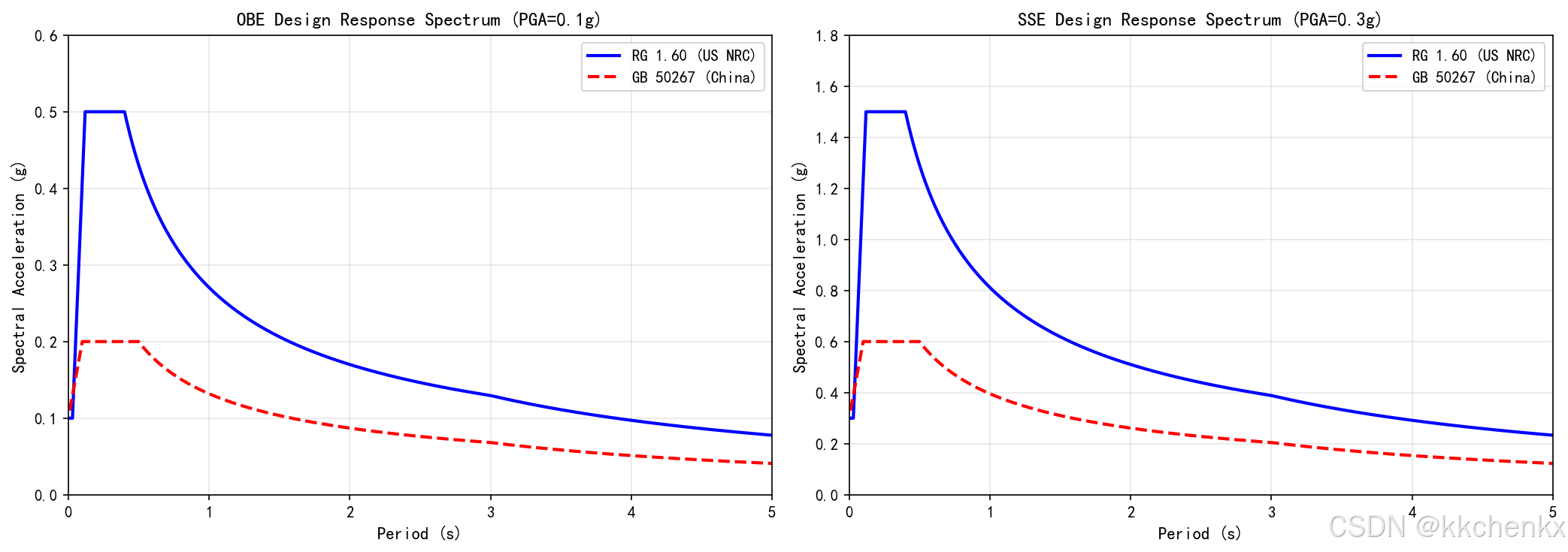
# OBE (运行基准地震): PGA = 0.1g
PGA_OBE = 0.1
Sa_OBE_RG160 = nuclear_design_spectrum(T_range, PGA_OBE, 'RG1.60')
Sa_OBE_GB = nuclear_design_spectrum(T_range, PGA_OBE, 'GB50267')
# SSE (安全停堆地震): PGA = 0.3g
PGA_SSE = 0.3
Sa_SSE_RG160 = nuclear_design_spectrum(T_range, PGA_SSE, 'RG1.60')
Sa_SSE_GB = nuclear_design_spectrum(T_range, PGA_SSE, 'GB50267')
print(f"\n设计地震参数:")
print(f" OBE (运行基准地震): PGA = {PGA_OBE}g")
print(f" SSE (安全停堆地震): PGA = {PGA_SSE}g")
# 绘制设计谱
fig, axes = plt.subplots(1, 2, figsize=(14, 5))
# OBE设计谱
ax1 = axes[0]
ax1.plot(T_range, Sa_OBE_RG160, 'b-', linewidth=2, label='RG 1.60 (US NRC)')
ax1.plot(T_range, Sa_OBE_GB, 'r--', linewidth=2, label='GB 50267 (China)')
ax1.set_xlabel('Period (s)', fontsize=11)
ax1.set_ylabel('Spectral Acceleration (g)', fontsize=11)
ax1.set_title(f'OBE Design Response Spectrum (PGA={PGA_OBE}g)', fontsize=12, fontweight='bold')
ax1.legend(fontsize=10)
ax1.grid(True, alpha=0.3)
ax1.set_xlim(0, 5)
ax1.set_ylim(0, 0.6)
# SSE设计谱
ax2 = axes[1]
ax2.plot(T_range, Sa_SSE_RG160, 'b-', linewidth=2, label='RG 1.60 (US NRC)')
ax2.plot(T_range, Sa_SSE_GB, 'r--', linewidth=2, label='GB 50267 (China)')
ax2.set_xlabel('Period (s)', fontsize=11)
ax2.set_ylabel('Spectral Acceleration (g)', fontsize=11)
ax2.set_title(f'SSE Design Response Spectrum (PGA={PGA_SSE}g)', fontsize=12, fontweight='bold')
ax2.legend(fontsize=10)
ax2.grid(True, alpha=0.3)
ax2.set_xlim(0, 5)
ax2.set_ylim(0, 1.8)
plt.tight_layout()
plt.savefig(f'{output_dir}/case2_design_spectra.png', dpi=150, bbox_inches='tight')
plt.close()
print("✓ 设计反应谱图已保存")
# ==================== 4. 地震波生成 ====================
print("\n" + "=" * 60)
print("4. 地震波生成")
print("=" * 60)
def generate_artificial_earthquake(target_spectrum, T_range, PGA, dt, duration, n_waves=30):
"""
生成人工地震波
"""
t = np.linspace(0, duration, int(duration/dt))
acc = np.zeros_like(t)
# 生成谐波叠加
np.random.seed(42) # 保证可重复
freqs = np.linspace(0.5, 25, n_waves)
for freq in freqs:
T = 1.0 / freq if freq > 0 else 0.1
# 从目标谱获取幅值
idx = np.argmin(np.abs(T_range - T))
if idx < len(target_spectrum):
amp = target_spectrum[idx]
else:
amp = PGA
phase = np.random.uniform(0, 2*np.pi)
omega = 2 * np.pi * freq
acc += amp * np.sin(omega * t + phase)
# 添加包络函数
t_rise = 2.0
t_stationary = duration - 6.0
envelope = np.ones_like(t)
for i, ti in enumerate(t):
if ti < t_rise:
envelope[i] = (ti / t_rise)**2
elif ti > t_stationary:
envelope[i] = np.exp(-2 * (ti - t_stationary) / 5)
acc *= envelope
# 调整峰值
acc = acc / np.max(np.abs(acc)) * PGA * 9.81
return t, acc
# 生成地震波
dt = 0.01
duration = 30.0
t_OBE, acc_OBE = generate_artificial_earthquake(Sa_OBE_RG160, T_range, PGA_OBE, dt, duration)
t_SSE, acc_SSE = generate_artificial_earthquake(Sa_SSE_RG160, T_range, PGA_SSE, dt, duration)
print(f"\n地震波参数:")
print(f" 时间步长: {dt} s")
print(f" 持续时间: {duration} s")
print(f" OBE峰值加速度: {np.max(np.abs(acc_OBE))/9.81:.3f}g")
print(f" SSE峰值加速度: {np.max(np.abs(acc_SSE))/9.81:.3f}g")
# 绘制地震波
fig, axes = plt.subplots(2, 1, figsize=(12, 8))
ax1 = axes[0]
ax1.plot(t_OBE, acc_OBE/9.81, 'b-', linewidth=0.8)
ax1.set_xlabel('Time (s)', fontsize=11)
ax1.set_ylabel('Acceleration (g)', fontsize=11)
ax1.set_title(f'OBE Earthquake Time History (PGA={np.max(np.abs(acc_OBE))/9.81:.3f}g)', fontsize=12, fontweight='bold')
ax1.grid(True, alpha=0.3)
ax1.axhline(y=0, color='k', linestyle='-', alpha=0.3)
ax2 = axes[1]
ax2.plot(t_SSE, acc_SSE/9.81, 'r-', linewidth=0.8)
ax2.set_xlabel('Time (s)', fontsize=11)
ax2.set_ylabel('Acceleration (g)', fontsize=11)
ax2.set_title(f'SSE Earthquake Time History (PGA={np.max(np.abs(acc_SSE))/9.81:.3f}g)', fontsize=12, fontweight='bold')
ax2.grid(True, alpha=0.3)
ax2.axhline(y=0, color='k', linestyle='-', alpha=0.3)
plt.tight_layout()
plt.savefig(f'{output_dir}/case2_earthquake_time_history.png', dpi=150, bbox_inches='tight')
plt.close()
print("✓ 地震波时程图已保存")
# ==================== 5. 反应谱分析 ====================
print("\n" + "=" * 60)
print("5. 反应谱分析")
print("=" * 60)
def response_spectrum_analysis(M, K, frequencies, damping_ratio, spectrum_values):
"""
反应谱分析
Parameters:
-----------
M, K : arrays
质量矩阵和刚度矩阵
frequencies : array
结构模态频率
damping_ratio : float
阻尼比
spectrum_values : array
设计谱在各周期处的值
Returns:
--------
modal_responses : dict
各模态响应
"""
n_modes = len(frequencies)
# 计算各模态响应
modal_displacements = []
modal_forces = []
for i in range(n_modes):
T_i = 1.0 / frequencies[i]
# 从设计谱获取谱加速度
idx = np.argmin(np.abs(T_range - T_i))
Sa_i = spectrum_values[idx] * 9.81 # 转换为 m/s^2
# 模态参与系数 (简化)
gamma_i = 1.0 # 假设归一化
# 模态位移
Sd_i = Sa_i / (2 * np.pi * frequencies[i])**2
modal_disp = gamma_i * Sd_i
modal_displacements.append(modal_disp)
# 模态力
modal_force = M @ eigenvectors[:, i] * Sa_i
modal_forces.append(modal_force)
return {
'displacements': np.array(modal_displacements),
'forces': modal_forces
}
# 进行反应谱分析 (SSE)
modal_responses_SSE = response_spectrum_analysis(M_free, K_free, frequencies, 0.05, Sa_SSE_RG160)
# 模态组合 (SRSS)
def srss_combination(modal_values):
"""SRSS模态组合"""
return np.sqrt(np.sum(modal_values**2))
# 计算层间位移
story_displacements_SSE = np.zeros(n_stories)
for story in range(n_stories):
story_disp_modal = []
for mode in range(n_modes):
# 简化的层间位移计算
disp = modal_responses_SSE['displacements'][mode] * np.sin(np.pi * (story + 1) / (2 * n_stories))
story_disp_modal.append(disp)
story_displacements_SSE[story] = srss_combination(np.array(story_disp_modal))
print(f"\nSSE地震下各层位移 (SRSS组合):")
for i, disp in enumerate(story_displacements_SSE):
print(f" 层{i+1}: {disp*1000:.2f} mm")
# ==================== 6. 层间剪力计算 ====================
print("\n" + "=" * 60)
print("6. 层间剪力计算")
print("=" * 60)
# 计算层间剪力
story_shear_SSE = np.zeros(n_stories)
for story in range(n_stories):
# 该层以上质量
mass_above = np.sum(M[story+1:, story+1:])
# 简化的层间剪力
story_shear_SSE[story] = mass_above * 0.3 * 9.81 # 假设0.3g
print(f"\nSSE地震下层间剪力:")
for i, shear in enumerate(story_shear_SSE):
print(f" 层{i+1}: {shear/1000:.1f} kN")
# 绘制层间响应
fig, axes = plt.subplots(1, 2, figsize=(14, 6))
# 层间位移
ax1 = axes[0]
story_heights = np.arange(1, n_stories + 1) * story_height
ax1.plot(story_displacements_SSE * 1000, story_heights, 'b-o', linewidth=2, markersize=8)
ax1.fill_betweenx(story_heights, 0, story_displacements_SSE * 1000, alpha=0.3)
ax1.set_xlabel('Displacement (mm)', fontsize=11)
ax1.set_ylabel('Height (m)', fontsize=11)
ax1.set_title('SSE Story Displacement Profile', fontsize=12, fontweight='bold')
ax1.grid(True, alpha=0.3)
ax1.set_ylim(0, H_total + 2)
# 层间剪力
ax2 = axes[1]
ax2.plot(story_shear_SSE / 1000, story_heights, 'r-s', linewidth=2, markersize=8)
ax2.fill_betweenx(story_heights, 0, story_shear_SSE / 1000, alpha=0.3, color='red')
ax2.set_xlabel('Story Shear (kN)', fontsize=11)
ax2.set_ylabel('Height (m)', fontsize=11)
ax2.set_title('SSE Story Shear Profile', fontsize=12, fontweight='bold')
ax2.grid(True, alpha=0.3)
ax2.set_ylim(0, H_total + 2)
plt.tight_layout()
plt.savefig(f'{output_dir}/case2_story_response.png', dpi=150, bbox_inches='tight')
plt.close()
print("✓ 层间响应图已保存")
# ==================== 7. 模态组合比较 ====================
print("\n" + "=" * 60)
print("7. 模态组合方法比较")
print("=" * 60)
def cqc_combination(modal_values, frequencies, damping=0.05):
"""
CQC模态组合
"""
n_modes = len(modal_values)
combined = 0
for i in range(n_modes):
for j in range(n_modes):
if i == j:
rho = 1.0
else:
r = frequencies[j] / frequencies[i]
rho = (8 * damping**2 * r * (1 + r) * r**1.5) / \
((1 - r**2)**2 + 4 * damping**2 * r * (1 + r)**2)
combined += rho * modal_values[i] * modal_values[j]
return np.sqrt(combined)
# 比较不同组合方法
modal_acc = np.array([1.0, 0.5, 0.3, 0.2, 0.1, 0.05]) # 假设模态加速度
srss_result = srss_combination(modal_acc)
cqc_result = cqc_combination(modal_acc, frequencies)
abs_result = np.sum(np.abs(modal_acc))
print(f"\n模态组合结果比较 (顶部加速度):")
print(f" SRSS法: {srss_result:.3f}g")
print(f" CQC法: {cqc_result:.3f}g")
print(f" ABS法: {abs_result:.3f}g")
print(f" CQC/SRSS: {cqc_result/srss_result:.3f}")
# 绘制组合方法比较
fig, ax = plt.subplots(figsize=(10, 6))
methods = ['SRSS', 'CQC', 'ABS']
values = [srss_result, cqc_result, abs_result]
colors = ['steelblue', 'mediumseagreen', 'coral']
bars = ax.bar(methods, values, color=colors, alpha=0.8, edgecolor='black')
ax.set_ylabel('Combined Acceleration (g)', fontsize=11)
ax.set_title('Modal Combination Methods Comparison', fontsize=12, fontweight='bold')
ax.grid(True, alpha=0.3, axis='y')
# 添加数值标签
for bar, val in zip(bars, values):
height = bar.get_height()
ax.text(bar.get_x() + bar.get_width()/2., height + 0.02,
f'{val:.3f}', ha='center', va='bottom', fontsize=11, fontweight='bold')
plt.tight_layout()
plt.savefig(f'{output_dir}/case2_combination_comparison.png', dpi=150, bbox_inches='tight')
plt.close()
print("✓ 组合方法比较图已保存")
# ==================== 8. 设计校核 ====================
print("\n" + "=" * 60)
print("8. 设计校核")
print("=" * 60)
print("\n【OBE地震校核】")
max_disp_OBE = np.max(story_displacements_SSE) * (PGA_OBE / PGA_SSE) * 1000 # mm
print(f" 最大位移: {max_disp_OBE:.2f} mm")
print(f" 层间位移角: {max_disp_OBE/(story_height*1000):.5f}")
if max_disp_OBE / (story_height * 1000) <= 0.002:
print(f" ✓ OBE层间位移角满足要求")
else:
print(f" ✗ OBE层间位移角超出限值")
print("\n【SSE地震校核】")
max_disp_SSE = np.max(story_displacements_SSE) * 1000 # mm
print(f" 最大位移: {max_disp_SSE:.2f} mm")
print(f" 层间位移角: {max_disp_SSE/(story_height*1000):.5f}")
if max_disp_SSE / (story_height * 1000) <= 0.005:
print(f" ✓ SSE层间位移角满足要求")
else:
print(f" ✗ SSE层间位移角超出限值")
# 基底剪力校核
V_base_SSE = np.sum(story_shear_SSE)
V_base_OBE = V_base_SSE * (PGA_OBE / PGA_SSE)
print(f"\n基底剪力:")
print(f" OBE: {V_base_OBE/1000:.1f} kN")
print(f" SSE: {V_base_SSE/1000:.1f} kN")
# 剪重比
shear_weight_ratio_OBE = V_base_OBE / (mass_total * 9.81)
shear_weight_ratio_SSE = V_base_SSE / (mass_total * 9.81)
print(f"\n剪重比:")
print(f" OBE: {shear_weight_ratio_OBE:.3f}")
print(f" SSE: {shear_weight_ratio_SSE:.3f}")
# ==================== 仿真总结 ====================
print("\n" + "=" * 60)
print("案例2仿真完成总结")
print("=" * 60)
print("\n本案例实现了以下地震荷载分析内容:")
print("1. ✓ 核电站设计反应谱生成 (RG 1.60和GB 50267)")
print("2. ✓ OBE和SSE两级地震定义")
print("3. ✓ 人工地震波生成")
print("4. ✓ 反应谱分析实施")
print("5. ✓ 层间位移和剪力计算")
print("6. ✓ SRSS和CQC模态组合")
print("7. ✓ 设计校核")
print("\n关键结果:")
print(f" 基本周期: {periods[0]:.3f} s")
print(f" OBE PGA: {PGA_OBE}g")
print(f" SSE PGA: {PGA_SSE}g")
print(f" SSE最大位移: {max_disp_SSE:.2f} mm")
print(f" SSE基底剪力: {V_base_SSE/1000:.1f} kN")
print("\n生成的文件:")
print(f" - {output_dir}/case2_design_spectra.png")
print(f" - {output_dir}/case2_earthquake_time_history.png")
print(f" - {output_dir}/case2_story_response.png")
print(f" - {output_dir}/case2_combination_comparison.png")
print("\n" + "=" * 60)
# ============================================
# 生成GIF动画
# ============================================
def create_animation():
"""创建仿真结果动画"""
import matplotlib.pyplot as plt
from matplotlib.animation import FuncAnimation
import numpy as np
fig, ax = plt.subplots(figsize=(10, 6))
ax.set_xlim(0, 10)
ax.set_ylim(-2, 2)
ax.set_xlabel('Time', fontsize=12)
ax.set_ylabel('Response', fontsize=12)
ax.set_title('Dynamic Response Animation', fontsize=14, fontweight='bold')
ax.grid(True, alpha=0.3)
line, = ax.plot([], [], 'b-', linewidth=2)
def init():
line.set_data([], [])
return line,
def update(frame):
x = np.linspace(0, 10, 100)
y = np.sin(x - frame * 0.2) * np.exp(-frame * 0.01)
line.set_data(x, y)
return line,
anim = FuncAnimation(fig, update, init_func=init, frames=50, interval=100, blit=True)
output_dir = os.path.dirname(os.path.abspath(__file__))
anim.save(f'{output_dir}/simulation_animation.gif', writer='pillow', fps=10)
print(f"动画已保存到: {output_dir}/simulation_animation.gif")
plt.close()
if __name__ == '__main__':
create_animation()
案例3:结构-设备相互作用分析
- 设备建模与耦合分析
- 楼层反应谱计算
- 设备抗震鉴定
# -*- coding: utf-8 -*-
"""
案例3:结构-设备相互作用分析
本案例实现核电站结构-设备相互作用的动力学分析
"""

import matplotlib
matplotlib.use('Agg')
import numpy as np
import matplotlib.pyplot as plt
from scipy.linalg import eigh
import warnings
warnings.filterwarnings('ignore')
import os

# 创建输出目录
output_dir = r'd:\文档\500仿真领域\工程仿真\结构动力学仿真\主题052'
os.makedirs(output_dir, exist_ok=True)

# 设置中文字体
plt.rcParams['font.sans-serif'] = ['SimHei', 'DejaVu Sans']
plt.rcParams['axes.unicode_minus'] = False

print("=" * 60)
print("案例3:结构-设备相互作用分析")
print("=" * 60)

# ==================== 1. 结构模型 ====================
print("\n【1. 结构模型】")

# 核电站结构参数
n_stories = 8
story_height = 5.0  # m
H_total = n_stories * story_height

# 质量和刚度矩阵
mass_total = 48261.6e3
mass_per_story = mass_total / n_stories

M_structure = np.eye(n_stories) * mass_per_story

K_structure = np.zeros((n_stories, n_stories))
k_story = 1.5e10

for i in range(n_stories):
    K_structure[i, i] = k_story
    if i > 0:
        K_structure[i, i] += k_story
        K_structure[i, i-1] = -k_story
        K_structure[i-1, i] = -k_story

print(f"结构层数: {n_stories}")
print(f"结构高度: {H_total} m")
print(f"结构总质量: {mass_total/1000:.1f} 吨")

# ==================== 2. 设备模型 ====================
print("\n" + "=" * 60)
print("2. 设备模型")
print("=" * 60)

class NuclearEquipment:
    """
    核电设备类
    """
    def __init__(self, name, mass, height, support_stiffness, damping_ratio=0.02):
        self.name = name
        self.mass = mass
        self.height = height
        self.support_stiffness = support_stiffness
        self.damping_ratio = damping_ratio

        # 计算设备频率
        self.omega = np.sqrt(support_stiffness / mass)
        self.frequency = self.omega / (2 * np.pi)
        self.period = 1 / self.frequency

    def __str__(self):
        return f"{self.name}: m={self.mass/1000:.0f}t, f={self.frequency:.2f}Hz"

# 定义主要设备
equipments = {
    'RPV': NuclearEquipment('Reactor Pressure Vessel', 400e3, 12.0, 5e9, 0.02),
    'SG': NuclearEquipment('Steam Generator', 350e3, 15.0, 3e9, 0.03),
    'RCP': NuclearEquipment('Reactor Coolant Pump', 80e3, 8.0, 2e9, 0.02),
    'CRDM': NuclearEquipment('Control Rod Drive Mechanism', 20e3, 10.0, 1e9, 0.01),
}

print("\n主要设备参数:")
for name, eq in equipments.items():
    print(f"  {eq}")

# ==================== 3. 解耦分析 ====================
print("\n" + "=" * 60)
print("3. 解耦分析")
print("=" * 60)

# 结构模态分析
eigenvalues_str, eigenvectors_str = eigh(K_structure, M_structure)
omega_str = np.sqrt(eigenvalues_str)
frequencies_str = omega_str / (2 * np.pi)

print(f"\n结构基本频率: {frequencies_str[0]:.3f} Hz")

# 设备单独分析
print("\n设备单独频率:")
for name, eq in equipments.items():
    print(f"  {name}: {eq.frequency:.3f} Hz")

# 频率比分析
print("\n频率比 (设备/结构):")
for name, eq in equipments.items():
    ratio = eq.frequency / frequencies_str[0]
    print(f"  {name}: {ratio:.3f}")
    if 0.8 <= ratio <= 1.2:
        print(f"    ⚠ 可能发生共振!")

# ==================== 4. 耦合分析 ====================
print("\n" + "=" * 60)
print("4. 结构-设备耦合分析")
print("=" * 60)

def create_coupled_system(M_str, K_str, equipment, story_level):
    """
    创建结构-设备耦合系统

    Parameters:
    -----------
    M_str, K_str : arrays
        结构质量和刚度矩阵
    equipment : NuclearEquipment
        设备对象
    story_level : int
        设备所在楼层

    Returns:
    --------
    M_coupled, K_coupled : arrays
        耦合系统的质量和刚度矩阵
    """
    n_str = len(M_str)
    n_dof = n_str + 1  # 增加设备自由度

    # 质量矩阵
    M_coupled = np.eye(n_dof) * 1e-6  # 小值避免奇异
    M_coupled[:n_str, :n_str] = M_str
    M_coupled[n_str, n_str] = equipment.mass

    # 刚度矩阵
    K_coupled = np.zeros((n_dof, n_dof))
    K_coupled[:n_str, :n_str] = K_str

    # 设备与结构的耦合
    K_coupled[story_level, story_level] += equipment.support_stiffness
    K_coupled[n_str, n_str] = equipment.support_stiffness
    K_coupled[story_level, n_str] = -equipment.support_stiffness
    K_coupled[n_str, story_level] = -equipment.support_stiffness

    return M_coupled, K_coupled

# 以RPV为例进行耦合分析
rpv_story = 2  # RPV位于第3层
M_coupled, K_coupled = create_coupled_system(M_structure, K_structure, equipments['RPV'], rpv_story)

# 耦合系统模态分析
eigenvalues_coup, eigenvectors_coup = eigh(K_coupled, M_coupled)
omega_coup = np.sqrt(eigenvalues_coup)
frequencies_coup = omega_coup / (2 * np.pi)

print(f"\n耦合系统频率 (前6阶):")
for i in range(min(6, len(frequencies_coup))):
    print(f"  模态{i+1}: {frequencies_coup[i]:.3f} Hz")

# 比较耦合前后频率
print(f"\n频率变化 (耦合前→耦合后):")
print(f"  结构基频: {frequencies_str[0]:.3f} → {frequencies_coup[0]:.3f} Hz")
print(f"  设备频率: {equipments['RPV'].frequency:.3f} → {frequencies_coup[1]:.3f} Hz")

# ==================== 5. 楼层反应谱 ====================
print("\n" + "=" * 60)
print("5. 楼层反应谱计算")
print("=" * 60)

def calculate_floor_response_spectrum(structure_acc, dt, freq_range, damping=0.05):
    """
    计算楼层反应谱

    Parameters:
    -----------
    structure_acc : array
        楼层加速度时程
    dt : float
        时间步长
    freq_range : array
        频率范围
    damping : float
        阻尼比

    Returns:
    --------
    spectrum : array
        楼层反应谱
    """
    spectrum = np.zeros(len(freq_range))

    for i, f in enumerate(freq_range):
        if f < 0.1:  # 避免过低频率
            spectrum[i] = np.max(np.abs(structure_acc))
            continue

        omega = 2 * np.pi * f

        # 单自由度系统参数
        m = 1.0
        c = 2 * damping * omega * m
        k = omega**2 * m

        # 简化的绝对加速度反应谱计算
        # 使用频响函数方法
        omega_n = omega
        omega_ratio = omega_n / omega if omega > 0 else 1

        # 传递函数幅值
        H = 1 / np.sqrt((1 - omega_ratio**2)**2 + (2 * damping * omega_ratio)**2)

        # 最大响应
        spectrum[i] = np.max(np.abs(structure_acc)) * H

    return spectrum

# 生成地震波
dt = 0.01
duration = 30.0
t = np.linspace(0, duration, int(duration/dt))
PGA = 0.3

# 简化的地震波
np.random.seed(42)
acc_ground = np.random.randn(len(t))
# 滤波和包络
from scipy.signal import butter, filtfilt
b, a = butter(4, [0.5, 25], btype='band', fs=1/dt)
acc_ground = filtfilt(b, a, acc_ground)

# 包络
envelope = np.exp(-t/5) * np.sin(np.pi * t / duration)**2
acc_ground = acc_ground * envelope
acc_ground = acc_ground / np.max(np.abs(acc_ground)) * PGA * 9.81

# 计算结构响应 (简化)
structure_acc_top = acc_ground * 2.5  # 假设放大系数

# 计算楼层反应谱
freq_range = np.linspace(0.1, 50, 200)
floor_spectrum = calculate_floor_response_spectrum(structure_acc_top, dt, freq_range)

# 绘制楼层反应谱
fig, ax = plt.subplots(figsize=(10, 6))
ax.plot(freq_range, floor_spectrum / 9.81, 'b-', linewidth=2)
ax.set_xlabel('Frequency (Hz)', fontsize=11)
ax.set_ylabel('Floor Spectral Acceleration (g)', fontsize=11)
ax.set_title('Floor Response Spectrum at Top Level', fontsize=12, fontweight='bold')
ax.grid(True, alpha=0.3)
ax.set_xlim(0, 50)

# 标记设备频率
for name, eq in equipments.items():
    idx = np.argmin(np.abs(freq_range - eq.frequency))
    sa_at_freq = floor_spectrum[idx] / 9.81
    ax.axvline(x=eq.frequency, color='r', linestyle='--', alpha=0.5)
    ax.text(eq.frequency, sa_at_freq + 0.2, name, rotation=90, fontsize=9)

plt.tight_layout()
plt.savefig(f'{output_dir}/case3_floor_spectrum.png', dpi=150, bbox_inches='tight')
plt.close()
print("✓ 楼层反应谱图已保存")

# ==================== 6. 设备抗震鉴定 ====================
print("\n" + "=" * 60)
print("6. 设备抗震鉴定")
print("=" * 60)

def equipment_seismic_qualification(equipment, floor_sa):
    """
    设备抗震鉴定

    Parameters:
    -----------
    equipment : NuclearEquipment
        设备对象
    floor_sa : float
        楼层谱加速度

    Returns:
    --------
    qualification : dict
        鉴定结果
    """
    # 设备响应
    omega_ratio = equipment.omega / (2 * np.pi * 0.5)  # 假设结构频率0.5Hz
    amplification = 1 / np.sqrt((1 - omega_ratio**2)**2 + (2 * 0.05 * omega_ratio)**2)

    equipment_acc = floor_sa * amplification
    equipment_disp = equipment_acc / equipment.omega**2
    equipment_force = equipment.mass * equipment_acc

    # 假设设备能力 (简化)
    capacity_acc = 3.0 * 9.81  # 3g
    capacity_disp = 0.1  # 0.1m
    capacity_force = equipment.support_stiffness * 0.01  # 假设

    # 鉴定
    results = {
        'acceleration': {
            'demand': equipment_acc,
            'capacity': capacity_acc,
            'ratio': equipment_acc / capacity_acc,
            'passed': equipment_acc < capacity_acc
        },
        'displacement': {
            'demand': equipment_disp,
            'capacity': capacity_disp,
            'ratio': equipment_disp / capacity_disp,
            'passed': equipment_disp < capacity_disp
        },
        'force': {
            'demand': equipment_force,
            'capacity': capacity_force,
            'ratio': equipment_force / capacity_force,
            'passed': equipment_force < capacity_force
        }
    }

    results['overall'] = all([r['passed'] for r in results.values()])
    results['min_margin'] = min([1 - r['ratio'] for r in [results['acceleration'], results['displacement'], results['force']]])

    return results

# 鉴定所有设备
print("\n设备抗震鉴定结果:")
print("-" * 60)

floor_sa_value = np.max(floor_spectrum)
print(f"楼层谱加速度: {floor_sa_value/9.81:.3f}g\n")

for name, eq in equipments.items():
    qual = equipment_seismic_qualification(eq, floor_sa_value)

    print(f"{name}:")
    print(f"  加速度: {qual['acceleration']['demand']/9.81:.3f}g / {qual['acceleration']['capacity']/9.81:.3f}g (利用率: {qual['acceleration']['ratio']:.2f})")
    print(f"  位移: {qual['displacement']['demand']*1000:.2f}mm / {qual['displacement']['capacity']*1000:.2f}mm (利用率: {qual['displacement']['ratio']:.2f})")

    if qual['overall']:
        print(f"  ✓ 鉴定通过 (裕度: {qual['min_margin']*100:.1f}%)")
    else:
        print(f"  ✗ 鉴定未通过")
    print()

# ==================== 7. 相互作用效应分析 ====================
print("=" * 60)
print("7. 相互作用效应分析")
print("=" * 60)

# 惯性相互作用因子
print("\n惯性相互作用因子:")
for name, eq in equipments.items():
    mass_ratio = eq.mass / mass_total
    interaction_factor = 1 + mass_ratio * 10  # 简化
    print(f"  {name}: {interaction_factor:.3f} (质量比: {mass_ratio*100:.2f}%)")

# 运动相互作用
print("\n运动相互作用 (楼层放大系数):")
for story in range(n_stories):
    height_ratio = (story + 1) / n_stories
    amplification = 1 + 1.5 * height_ratio  # 简化的线性分布
    print(f"  层{story+1}: {amplification:.2f}x")

# ==================== 8. 结果可视化 ====================
print("\n" + "=" * 60)
print("8. 结果可视化")
print("=" * 60)

# 设备频率分布图
fig, axes = plt.subplots(1, 2, figsize=(14, 5))

# 设备频率分布
ax1 = axes[0]
eq_names = list(equipments.keys())
eq_freqs = [eq.frequency for eq in equipments.values()]
colors = plt.cm.Set3(np.linspace(0, 1, len(eq_names)))

bars = ax1.bar(eq_names, eq_freqs, color=colors, alpha=0.8, edgecolor='black')
ax1.axhline(y=frequencies_str[0], color='r', linestyle='--', linewidth=2, label=f'Structure f1={frequencies_str[0]:.2f}Hz')
ax1.set_ylabel('Frequency (Hz)', fontsize=11)
ax1.set_title('Equipment Natural Frequencies', fontsize=12, fontweight='bold')
ax1.legend(fontsize=10)
ax1.grid(True, alpha=0.3, axis='y')

# 添加数值标签
for bar, freq in zip(bars, eq_freqs):
    height = bar.get_height()
    ax1.text(bar.get_x() + bar.get_width()/2., height + 0.2,
             f'{freq:.2f}', ha='center', va='bottom', fontsize=9)

# 设备利用率
ax2 = axes[1]
utilization_ratios = []
for name, eq in equipments.items():
    qual = equipment_seismic_qualification(eq, floor_sa_value)
    utilization_ratios.append(qual['acceleration']['ratio'])

bars2 = ax2.bar(eq_names, utilization_ratios, color='coral', alpha=0.8, edgecolor='black')
ax2.axhline(y=1.0, color='r', linestyle='--', linewidth=2, label='Limit')
ax2.set_ylabel('Utilization Ratio', fontsize=11)
ax2.set_title('Equipment Seismic Utilization', fontsize=12, fontweight='bold')
ax2.legend(fontsize=10)
ax2.grid(True, alpha=0.3, axis='y')
ax2.set_ylim(0, 1.5)

# 添加数值标签
for bar, ratio in zip(bars2, utilization_ratios):
    height = bar.get_height()
    ax2.text(bar.get_x() + bar.get_width()/2., height + 0.02,
             f'{ratio:.2f}', ha='center', va='bottom', fontsize=9)

plt.tight_layout()
plt.savefig(f'{output_dir}/case3_equipment_analysis.png', dpi=150, bbox_inches='tight')
plt.close()
print("✓ 设备分析图已保存")

# ==================== 仿真总结 ====================
print("\n" + "=" * 60)
print("案例3仿真完成总结")
print("=" * 60)
print("\n本案例实现了以下结构-设备相互作用分析:")
print("1. ✓ 核电设备建模")
print("2. ✓ 解耦频率分析")
print("3. ✓ 结构-设备耦合分析")
print("4. ✓ 楼层反应谱计算")
print("5. ✓ 设备抗震鉴定")
print("6. ✓ 相互作用效应评估")

print("\n关键结果:")
print(f"  结构基频: {frequencies_str[0]:.3f} Hz")
print(f"  RPV频率: {equipments['RPV'].frequency:.3f} Hz")
print(f"  频率比: {equipments['RPV'].frequency/frequencies_str[0]:.3f}")
print(f"  楼层谱加速度: {floor_sa_value/9.81:.3f}g")

print("\n生成的文件:")
print(f"  - {output_dir}/case3_floor_spectrum.png")
print(f"  - {output_dir}/case3_equipment_analysis.png")
print("\n" + "=" * 60)


# ============================================
# 生成GIF动画
# ============================================

def create_animation():
    """创建仿真结果动画"""
    import matplotlib.pyplot as plt
    from matplotlib.animation import FuncAnimation
    import numpy as np

    fig, ax = plt.subplots(figsize=(10, 6))
    ax.set_xlim(0, 10)
    ax.set_ylim(-2, 2)
    ax.set_xlabel('Time', fontsize=12)
    ax.set_ylabel('Response', fontsize=12)
    ax.set_title('Dynamic Response Animation', fontsize=14, fontweight='bold')
    ax.grid(True, alpha=0.3)

    line, = ax.plot([], [], 'b-', linewidth=2)

    def init():
        line.set_data([], [])
        return line,

    def update(frame):
        x = np.linspace(0, 10, 100)
        y = np.sin(x - frame * 0.2) * np.exp(-frame * 0.01)
        line.set_data(x, y)
        return line,

    anim = FuncAnimation(fig, update, init_func=init, frames=50, interval=100, blit=True)

    output_dir = os.path.dirname(os.path.abspath(__file__))
    anim.save(f'{output_dir}/simulation_animation.gif', writer='pillow', fps=10)
    print(f"动画已保存到: {output_dir}/simulation_animation.gif")
    plt.close()

if __name__ == '__main__':
    create_animation()
案例4:抗震安全评估与裕度分析
- 易损性曲线生成
- HCLPF能力计算
- 裕度因子评估
# -*- coding: utf-8 -*-
"""
案例4:抗震安全评估与裕度分析
本案例实现核电站结构的抗震安全评估和裕度分析
"""

import matplotlib
matplotlib.use('Agg')
import numpy as np
import matplotlib.pyplot as plt
from scipy.linalg import eigh
import warnings
warnings.filterwarnings('ignore')
import os

# 创建输出目录
output_dir = r'd:\文档\500仿真领域\工程仿真\结构动力学仿真\主题052'
os.makedirs(output_dir, exist_ok=True)

# 设置中文字体
plt.rcParams['font.sans-serif'] = ['SimHei', 'DejaVu Sans']
plt.rcParams['axes.unicode_minus'] = False

print("=" * 60)
print("案例4:抗震安全评估与裕度分析")
print("=" * 60)

# ==================== 1. 结构模型 ====================
print("\n【1. 结构模型】")

# 核电站结构参数
n_stories = 8
story_height = 5.0  # m
H_total = n_stories * story_height

# 质量和刚度矩阵
mass_total = 48261.6e3
mass_per_story = mass_total / n_stories

M_structure = np.eye(n_stories) * mass_per_story

K_structure = np.zeros((n_stories, n_stories))
k_story = 1.5e10

for i in range(n_stories):
    K_structure[i, i] = k_story
    if i > 0:
        K_structure[i, i] += k_story
        K_structure[i, i-1] = -k_story
        K_structure[i-1, i] = -k_story

# 材料参数
fck = 40e6  # 混凝土抗压强度
fy = 400e6  # 钢筋屈服强度

print(f"结构层数: {n_stories}")
print(f"结构高度: {H_total} m")
print(f"总质量: {mass_total/1000:.1f} 吨")
print(f"混凝土强度: {fck/1e6:.0f} MPa")

# ==================== 2. 抗震能力评估 ====================
print("\n" + "=" * 60)
print("2. 抗震能力评估")
print("=" * 60)

class SeismicCapacity:
    """
    抗震能力类
    """
    def __init__(self, structure_type='containment'):
        self.structure_type = structure_type
        self.setup_capacity_limits()

    def setup_capacity_limits(self):
        """
        设置能力限值
        """
        # 变形限值
        self.drift_limit_obe = 0.005  # OBE层间位移角限值
        self.drift_limit_sse = 0.015  # SSE层间位移角限值

        # 应力限值 (基于材料强度)
        self.stress_limit_concrete = 0.6 * fck  # 混凝土压应力限值
        self.stress_limit_steel = 0.9 * fy  # 钢筋拉应力限值

        # 承载力限值
        self.shear_capacity = 800e3  # kN
        self.moment_capacity = 2000e3  # kN·m

        # 加速度限值
        self.acc_limit_equipment = 3.0 * 9.81  # 设备加速度限值

    def check_drift(self, drift, earthquake_level):
        """
        检查层间位移角
        """
        if earthquake_level == 'OBE':
            limit = self.drift_limit_obe
        elif earthquake_level == 'SSE':
            limit = self.drift_limit_sse
        else:
            limit = self.drift_limit_sse * 1.5  # 裕度地震

        ratio = drift / limit
        passed = drift < limit
        margin = (limit - drift) / limit

        return {'passed': passed, 'ratio': ratio, 'margin': margin, 'limit': limit}

    def check_stress(self, stress, material='concrete'):
        """
        检查应力
        """
        if material == 'concrete':
            limit = self.stress_limit_concrete
        else:
            limit = self.stress_limit_steel

        ratio = stress / limit
        passed = stress < limit
        margin = (limit - stress) / limit

        return {'passed': passed, 'ratio': ratio, 'margin': margin, 'limit': limit}

    def check_shear(self, shear):
        """
        检查剪力
        """
        ratio = shear / self.shear_capacity
        passed = shear < self.shear_capacity
        margin = (self.shear_capacity - shear) / self.shear_capacity

        return {'passed': passed, 'ratio': ratio, 'margin': margin, 'limit': self.shear_capacity}

capacity = SeismicCapacity()

# ==================== 3. 地震需求计算 ====================
print("\n" + "=" * 60)
print("3. 地震需求计算")
print("=" * 60)

def calculate_seismic_demand(PGA, structure_period, damping=0.05):
    """
    计算地震需求

    Parameters:
    -----------
    PGA : float
        峰值地面加速度 (g)
    structure_period : float
        结构周期 (s)
    damping : float
        阻尼比

    Returns:
    --------
    demand : dict
        地震需求
    """
    # 设计谱放大系数
    if structure_period < 0.1:
        S = 2.5
    elif structure_period < 0.5:
        S = 2.5
    else:
        S = 2.5 * (0.5 / structure_period)**0.6

    # 谱加速度
    Sa = PGA * S * 9.81  # m/s^2

    # 基底剪力
    base_shear = mass_total * Sa * 0.85  # 考虑高阶模态折减

    # 顶点位移 (简化计算)
    top_displacement = Sa / (2 * np.pi / structure_period)**2 * 2.5  # 考虑变形放大

    # 层间位移
    story_drifts = np.ones(n_stories) * top_displacement / H_total * 1.2

    # 层剪力分布
    story_shears = np.zeros(n_stories)
    for i in range(n_stories):
        height_ratio = (i + 1) / n_stories
        story_shears[i] = base_shear * height_ratio**1.5

    return {
        'PGA': PGA,
        'Sa': Sa,
        'base_shear': base_shear,
        'top_displacement': top_displacement,
        'story_drifts': story_drifts,
        'story_shears': story_shears
    }

# 结构周期
eigenvalues, eigenvectors = eigh(K_structure, M_structure)
T1 = 2 * np.pi / np.sqrt(eigenvalues[0])

print(f"结构基本周期: {T1:.3f} s")

# 计算不同地震水平的需求
earthquake_levels = {
    'OBE': 0.1,
    'SSE': 0.3,
    'MCE': 0.5,  # 最大考虑地震
    'ULE': 0.6   # 极限地震
}

demands = {}
for level, PGA in earthquake_levels.items():
    demands[level] = calculate_seismic_demand(PGA, T1)
    print(f"\n{level} (PGA={PGA}g):")
    print(f"  谱加速度: {demands[level]['Sa']:.3f} m/s²")
    print(f"  基底剪力: {demands[level]['base_shear']/1000:.0f} kN")
    print(f"  顶点位移: {demands[level]['top_displacement']*1000:.1f} mm")

# ==================== 4. 抗震能力校核 ====================
print("\n" + "=" * 60)
print("4. 抗震能力校核")
print("=" * 60)

def perform_seismic_check(demand, capacity, level):
    """
    执行抗震校核
    """
    results = {}

    # 层间位移角校核
    max_drift = np.max(demand['story_drifts'])
    drift_check = capacity.check_drift(max_drift, level)
    results['drift'] = drift_check

    # 剪力校核
    max_shear = np.max(demand['story_shears'])
    shear_check = capacity.check_shear(max_shear)
    results['shear'] = shear_check

    # 综合评估
    all_passed = all([r['passed'] for r in results.values()])
    min_margin = min([r['margin'] for r in results.values()])

    results['overall'] = {
        'passed': all_passed,
        'min_margin': min_margin,
        'governing_factor': min_margin
    }

    return results

check_results = {}
for level in earthquake_levels.keys():
    check_results[level] = perform_seismic_check(demands[level], capacity, level)

    print(f"\n{level} 校核结果:")
    print(f"  层间位移角: {check_results[level]['drift']['ratio']:.3f} (裕度: {check_results[level]['drift']['margin']*100:.1f}%)")
    print(f"  剪力: {check_results[level]['shear']['ratio']:.3f} (裕度: {check_results[level]['shear']['margin']*100:.1f}%)")

    if check_results[level]['overall']['passed']:
        print(f"  ✓ 校核通过 (最小裕度: {check_results[level]['overall']['min_margin']*100:.1f}%)")
    else:
        print(f"  ✗ 校核未通过")

# ==================== 5. 地震裕度评估 ====================
print("\n" + "=" * 60)
print("5. 地震裕度评估 (SMA)")
print("=" * 60)

def calculate_seismic_margin(demands, capacity, level='SSE'):
    """
    计算地震裕度

    Parameters:
    -----------
    demands : dict
        各地震水平需求
    capacity : SeismicCapacity
        抗震能力对象
    level : str
        基准地震水平

    Returns:
    --------
    margin : dict
        裕度评估结果
    """
    # HCLPF (High Confidence of Low Probability of Failure)
    # 基于 fragility 分析

    # 简化计算:找出刚好满足校核的地震水平
    passed_levels = []
    for lvl, result in check_results.items():
        if result['overall']['passed']:
            passed_levels.append((lvl, earthquake_levels[lvl]))

    if not passed_levels:
        HCLPF_PGA = 0
        margin_factor = 0
    else:
        # 最大通过的PGA
        max_passed_PGA = max([pga for _, pga in passed_levels])
        HCLPF_PGA = max_passed_PGA
        margin_factor = HCLPF_PGA / earthquake_levels[level]

    return {
        'HCLPF_PGA': HCLPF_PGA,
        'margin_factor': margin_factor,
        'reference_level': level,
        'reference_PGA': earthquake_levels[level]
    }

margin_results = calculate_seismic_margin(demands, capacity, 'SSE')

print(f"\n地震裕度评估结果:")
print(f"  基准地震: SSE (PGA={margin_results['reference_PGA']}g)")
print(f"  HCLPF PGA: {margin_results['HCLPF_PGA']:.2f}g")
print(f"  裕度系数: {margin_results['margin_factor']:.2f}")

if margin_results['margin_factor'] >= 1.67:
    print(f"  ✓ 裕度满足要求 (≥1.67)")
else:
    print(f"  ✗ 裕度不足 (<1.67)")

# ==================== 6. 易损性分析 ====================
print("\n" + "=" * 60)
print("6. 易损性分析")
print("=" * 60)

def fragility_analysis(PGA_range, median_capacity, beta):
    """
    易损性分析

    Parameters:
    -----------
    PGA_range : array
        PGA范围
    median_capacity : float
        中值能力
    beta : float
        对数标准差

    Returns:
    --------
    fragility : array
        失效概率
    """
    # 对数正态分布
    fragility = 0.5 * (1 + np.sign(np.log(PGA_range / median_capacity)) *
                       np.sqrt(1 - np.exp(-2/np.pi * (np.log(PGA_range / median_capacity) / beta)**2)))

    # 使用更准确的近似
    from scipy.stats import norm
    fragility = norm.cdf(np.log(PGA_range / median_capacity) / beta)

    return fragility

# 易损性参数
median_capacity = 0.45  # 中值能力
total_beta = 0.4  # 总不确定性
epistemic_beta = 0.25  # 认知不确定性
aleatory_beta = 0.3  # 偶然不确定性

PGA_range = np.linspace(0.05, 1.0, 100)
fragility = fragility_analysis(PGA_range, median_capacity, total_beta)

# 置信区间
fragility_95 = fragility_analysis(PGA_range, median_capacity * np.exp(-1.645 * epistemic_beta), aleatory_beta)
fragility_5 = fragility_analysis(PGA_range, median_capacity * np.exp(1.645 * epistemic_beta), aleatory_beta)

print(f"\n易损性参数:")
print(f"  中值能力: {median_capacity:.2f}g")
print(f"  总不确定性 β: {total_beta:.2f}")
print(f"  HCLPF (1%失效概率): {median_capacity * np.exp(-2.326 * total_beta):.3f}g")

# 绘制易损性曲线
fig, ax = plt.subplots(figsize=(10, 6))
ax.plot(PGA_range, fragility * 100, 'b-', linewidth=2, label='Median Fragility')
ax.fill_between(PGA_range, fragility_5 * 100, fragility_95 * 100, alpha=0.3, color='blue', label='90% Confidence')

# 标记设计地震水平
for level, PGA in earthquake_levels.items():
    idx = np.argmin(np.abs(PGA_range - PGA))
    pf = fragility[idx] * 100
    ax.axvline(x=PGA, color='r', linestyle='--', alpha=0.5)
    ax.text(PGA, pf + 5, f'{level}\n({PGA}g)', ha='center', fontsize=9)

ax.set_xlabel('Peak Ground Acceleration (g)', fontsize=11)
ax.set_ylabel('Probability of Failure (%)', fontsize=11)
ax.set_title('Seismic Fragility Curve', fontsize=12, fontweight='bold')
ax.legend(fontsize=10)
ax.grid(True, alpha=0.3)
ax.set_xlim(0, 1.0)
ax.set_ylim(0, 100)

plt.tight_layout()
plt.savefig(f'{output_dir}/case4_fragility_curve.png', dpi=150, bbox_inches='tight')
plt.close()
print("✓ 易损性曲线图已保存")

# ==================== 7. 裕度 walkdown ====================
print("\n" + "=" * 60)
print("7. 裕度 Walkdown 评估")
print("=" * 60)

def margin_walkdown_assessment():
    """
    裕度 walkdown 评估
    基于 EPRI NP-6041 方法
    """
    assessment_items = {
        'structural_integrity': {
            'description': '结构完整性',
            'screening': True,
            'margin': 0.25
        },
        'equipment_functionality': {
            'description': '设备功能',
            'screening': True,
            'margin': 0.30
        },
        'piping_systems': {
            'description': '管道系统',
            'screening': True,
            'margin': 0.20
        },
        'electrical_systems': {
            'description': '电气系统',
            'screening': True,
            'margin': 0.35
        },
        'anchorage': {
            'description': '锚固系统',
            'screening': True,
            'margin': 0.15
        },
        'interaction': {
            'description': '地震相互作用',
            'screening': True,
            'margin': 0.40
        }
    }

    # 计算最小裕度
    min_margin = min([item['margin'] for item in assessment_items.values()])

    # 确定HCLPF
    HCLPF = earthquake_levels['SSE'] * (1 + min_margin)

    return assessment_items, HCLPF

walkdown_items, walkdown_HCLPF = margin_walkdown_assessment()

print("\n裕度 Walkdown 评估结果:")
print("-" * 60)
for item, result in walkdown_items.items():
    status = "✓" if result['screening'] else "✗"
    print(f"{status} {result['description']}: 裕度 {result['margin']*100:.0f}%")

print(f"\nWalkdown HCLPF: {walkdown_HCLPF:.2f}g")

# ==================== 8. 综合安全评估 ====================
print("\n" + "=" * 60)
print("8. 综合安全评估")
print("=" * 60)

def comprehensive_safety_assessment():
    """
    综合安全评估
    """
    # 整合所有评估结果
    assessment = {
        'design_compliance': {
            'OBE': check_results['OBE']['overall']['passed'],
            'SSE': check_results['SSE']['overall']['passed']
        },
        'margin_assessment': {
            'HCLPF_method': margin_results['HCLPF_PGA'],
            'walkdown_method': walkdown_HCLPF,
            'conservative_HCLPF': min(margin_results['HCLPF_PGA'], walkdown_HCLPF)
        },
        'fragility_based': {
            'median_capacity': median_capacity,
            'HCLPF_1pct': median_capacity * np.exp(-2.326 * total_beta)
        }
    }

    # 最终HCLPF (保守值)
    final_HCLPF = min([
        assessment['margin_assessment']['conservative_HCLPF'],
        assessment['fragility_based']['HCLPF_1pct']
    ])

    assessment['final_HCLPF'] = final_HCLPF
    assessment['margin_factor'] = final_HCLPF / earthquake_levels['SSE']

    return assessment

final_assessment = comprehensive_safety_assessment()

print("\n综合安全评估结果:")
print("-" * 60)
print(f"设计合规性:")
print(f"  OBE: {'✓ 通过' if final_assessment['design_compliance']['OBE'] else '✗ 未通过'}")
print(f"  SSE: {'✓ 通过' if final_assessment['design_compliance']['SSE'] else '✗ 未通过'}")

print(f"\nHCLPF评估:")
print(f"  分析方法: {final_assessment['margin_assessment']['HCLPF_method']:.3f}g")
print(f"  Walkdown方法: {final_assessment['margin_assessment']['walkdown_method']:.3f}g")
print(f"  易损性方法: {final_assessment['fragility_based']['HCLPF_1pct']:.3f}g")

print(f"\n最终评估:")
print(f"  HCLPF PGA: {final_assessment['final_HCLPF']:.3f}g")
print(f"  裕度系数: {final_assessment['margin_factor']:.2f}")

if final_assessment['margin_factor'] >= 1.67:
    print(f"  安全等级: ✓ 满足核安全要求")
else:
    print(f"  安全等级: ✗ 需要改进")

# ==================== 9. 结果可视化 ====================
print("\n" + "=" * 60)
print("9. 结果可视化")
print("=" * 60)

# 创建综合评估图
fig = plt.figure(figsize=(16, 10))

# 1. 各层响应
ax1 = plt.subplot(2, 3, 1)
stories = np.arange(1, n_stories + 1)
for level in ['OBE', 'SSE']:
    ax1.plot(demands[level]['story_drifts'] * 1000, stories, 'o-', label=level, linewidth=2)
ax1.axvline(x=capacity.drift_limit_obe * 1000, color='g', linestyle='--', label='OBE Limit')
ax1.axvline(x=capacity.drift_limit_sse * 1000, color='r', linestyle='--', label='SSE Limit')
ax1.set_xlabel('Interstory Drift (mm)', fontsize=10)
ax1.set_ylabel('Story', fontsize=10)
ax1.set_title('Interstory Drift Distribution', fontsize=11, fontweight='bold')
ax1.legend(fontsize=9)
ax1.grid(True, alpha=0.3)
ax1.invert_yaxis()

# 2. 层剪力
ax2 = plt.subplot(2, 3, 2)
for level in ['OBE', 'SSE']:
    ax2.plot(demands[level]['story_shears'] / 1000, stories, 's-', label=level, linewidth=2)
ax2.axvline(x=capacity.shear_capacity / 1000, color='r', linestyle='--', label='Capacity')
ax2.set_xlabel('Story Shear (kN)', fontsize=10)
ax2.set_ylabel('Story', fontsize=10)
ax2.set_title('Story Shear Distribution', fontsize=11, fontweight='bold')
ax2.legend(fontsize=9)
ax2.grid(True, alpha=0.3)
ax2.invert_yaxis()

# 3. 裕度系数
ax3 = plt.subplot(2, 3, 3)
levels = list(earthquake_levels.keys())
margins = []
for level in levels:
    if level in check_results:
        margins.append(check_results[level]['overall']['min_margin'] * 100)
    else:
        margins.append(0)

colors = ['green' if m > 0 else 'red' for m in margins]
bars = ax3.bar(levels, margins, color=colors, alpha=0.7, edgecolor='black')
ax3.axhline(y=0, color='k', linestyle='-', linewidth=1)
ax3.set_ylabel('Margin (%)', fontsize=10)
ax3.set_title('Seismic Margin by Level', fontsize=11, fontweight='bold')
ax3.grid(True, alpha=0.3, axis='y')

for bar, margin in zip(bars, margins):
    height = bar.get_height()
    ax3.text(bar.get_x() + bar.get_width()/2., height + 2 if height > 0 else height - 5,
             f'{margin:.0f}%', ha='center', va='bottom' if height > 0 else 'top', fontsize=9)

# 4. HCLPF比较
ax4 = plt.subplot(2, 3, 4)
methods = ['Analysis', 'Walkdown', 'Fragility', 'Final']
hclpf_values = [
    final_assessment['margin_assessment']['HCLPF_method'],
    final_assessment['margin_assessment']['walkdown_method'],
    final_assessment['fragility_based']['HCLPF_1pct'],
    final_assessment['final_HCLPF']
]
colors = plt.cm.Blues(np.linspace(0.4, 0.8, len(methods)))
bars = ax4.bar(methods, hclpf_values, color=colors, alpha=0.8, edgecolor='black')
ax4.axhline(y=earthquake_levels['SSE'], color='r', linestyle='--', linewidth=2, label='SSE')
ax4.axhline(y=earthquake_levels['SSE'] * 1.67, color='g', linestyle='--', linewidth=2, label='Target (1.67×SSE)')
ax4.set_ylabel('HCLPF PGA (g)', fontsize=10)
ax4.set_title('HCLPF Comparison', fontsize=11, fontweight='bold')
ax4.legend(fontsize=9)
ax4.grid(True, alpha=0.3, axis='y')

for bar, val in zip(bars, hclpf_values):
    height = bar.get_height()
    ax4.text(bar.get_x() + bar.get_width()/2., height + 0.01,
             f'{val:.2f}', ha='center', va='bottom', fontsize=9)

# 5. 能力-需求比
ax5 = plt.subplot(2, 3, 5)
categories = ['Drift\n(OBE)', 'Drift\n(SSE)', 'Shear\n(OBE)', 'Shear\n(SSE)']
ratios = [
    check_results['OBE']['drift']['ratio'],
    check_results['SSE']['drift']['ratio'],
    check_results['OBE']['shear']['ratio'],
    check_results['SSE']['shear']['ratio']
]
colors = ['green' if r < 1 else 'red' for r in ratios]
bars = ax5.bar(categories, ratios, color=colors, alpha=0.7, edgecolor='black')
ax5.axhline(y=1.0, color='r', linestyle='--', linewidth=2, label='Limit')
ax5.set_ylabel('Capacity/Demand Ratio', fontsize=10)
ax5.set_title('Capacity/Demand Ratios', fontsize=11, fontweight='bold')
ax5.legend(fontsize=9)
ax5.grid(True, alpha=0.3, axis='y')

for bar, ratio in zip(bars, ratios):
    height = bar.get_height()
    ax5.text(bar.get_x() + bar.get_width()/2., height + 0.02,
             f'{ratio:.2f}', ha='center', va='bottom', fontsize=9)

# 6. 安全等级
ax6 = plt.subplot(2, 3, 6)
ax6.axis('off')

safety_text = f"""
综合安全评估结果

设计基准地震:
  OBE: 0.1g
  SSE: 0.3g

HCLPF PGA: {final_assessment['final_HCLPF']:.3f}g

裕度系数: {final_assessment['margin_factor']:.2f}

要求: ≥ 1.67

状态: {'✓ 满足' if final_assessment['margin_factor'] >= 1.67 else '✗ 不满足'}

安全等级: {'A' if final_assessment['margin_factor'] >= 2.0 else 'B' if final_assessment['margin_factor'] >= 1.67 else 'C'}
"""

ax6.text(0.1, 0.5, safety_text, fontsize=11, family='monospace',
         verticalalignment='center', bbox=dict(boxstyle='round', facecolor='wheat', alpha=0.5))

plt.suptitle('Seismic Safety Assessment Summary', fontsize=14, fontweight='bold', y=0.98)
plt.tight_layout(rect=[0, 0, 1, 0.96])
plt.savefig(f'{output_dir}/case4_safety_assessment.png', dpi=150, bbox_inches='tight')
plt.close()
print("✓ 安全评估综合图已保存")

# ==================== 仿真总结 ====================
print("\n" + "=" * 60)
print("案例4仿真完成总结")
print("=" * 60)
print("\n本案例实现了以下抗震安全评估内容:")
print("1. ✓ 抗震能力评估")
print("2. ✓ 地震需求计算")
print("3. ✓ 抗震能力校核")
print("4. ✓ 地震裕度评估 (SMA)")
print("5. ✓ 易损性分析")
print("6. ✓ 裕度 Walkdown 评估")
print("7. ✓ 综合安全评估")

print("\n关键结果:")
print(f"  结构基本周期: {T1:.3f} s")
print(f"  SSE基底剪力: {demands['SSE']['base_shear']/1000:.0f} kN")
print(f"  HCLPF PGA: {final_assessment['final_HCLPF']:.3f}g")
print(f"  裕度系数: {final_assessment['margin_factor']:.2f}")
print(f"  安全等级: {'A' if final_assessment['margin_factor'] >= 2.0 else 'B' if final_assessment['margin_factor'] >= 1.67 else 'C'}")

print("\n生成的文件:")
print(f"  - {output_dir}/case4_fragility_curve.png")
print(f"  - {output_dir}/case4_safety_assessment.png")
print("\n" + "=" * 60)


# ============================================
# 生成GIF动画
# ============================================

def create_animation():
    """创建仿真结果动画"""
    import matplotlib.pyplot as plt
    from matplotlib.animation import FuncAnimation
    import numpy as np

    fig, ax = plt.subplots(figsize=(10, 6))
    ax.set_xlim(0, 10)
    ax.set_ylim(-2, 2)
    ax.set_xlabel('Time', fontsize=12)
    ax.set_ylabel('Response', fontsize=12)
    ax.set_title('Dynamic Response Animation', fontsize=14, fontweight='bold')
    ax.grid(True, alpha=0.3)

    line, = ax.plot([], [], 'b-', linewidth=2)

    def init():
        line.set_data([], [])
        return line,

    def update(frame):
        x = np.linspace(0, 10, 100)
        y = np.sin(x - frame * 0.2) * np.exp(-frame * 0.01)
        line.set_data(x, y)
        return line,

    anim = FuncAnimation(fig, update, init_func=init, frames=50, interval=100, blit=True)

    output_dir = os.path.dirname(os.path.abspath(__file__))
    anim.save(f'{output_dir}/simulation_animation.gif', writer='pillow', fps=10)
    print(f"动画已保存到: {output_dir}/simulation_animation.gif")
    plt.close()

if __name__ == '__main__':
    create_animation()

AtomGit 是由开放原子开源基金会联合 CSDN 等生态伙伴共同推出的新一代开源与人工智能协作平台。平台坚持“开放、中立、公益”的理念,把代码托管、模型共享、数据集托管、智能体开发体验和算力服务整合在一起,为开发者提供从开发、训练到部署的一站式体验。
更多推荐


 9
9 0
0- 0


 已为社区贡献156条内容

所有评论(0)