主题033：电磁场仿真不确定性量化

引言

在工程实践中，电磁装置的输入参数往往存在不确定性：材料属性的制造公差、几何尺寸的加工误差、环境温度的波动等。这些不确定性会传播到系统输出，影响产品性能和可靠性。不确定性量化（Uncertainty Quantification, UQ）正是研究如何表征、传播和管理这些不确定性的科学。

本教程将系统介绍不确定性量化在电磁场仿真中的核心方法：

1. 蒙特卡洛方法：基于随机采样的统计模拟
2. 多项式混沌展开（PCE）：高效的代理模型方法
3. 灵敏度分析：识别关键不确定性来源
4. 可靠性分析：评估系统满足性能要求的概率

通过学习本教程，您将掌握如何量化电磁设计中的不确定性，做出更稳健的工程决策。

---

1. 不确定性来源与分类

1.1 不确定性类型

** aleatory不确定性（偶然不确定性）**：

• 本质随机性，不可消除
• 示例：材料微观结构的随机分布、环境噪声
• 建模：概率分布

** epistemic不确定性（认知不确定性）**：

• 知识缺乏导致，可减少
• 示例：模型简化假设、参数测量误差
• 建模：区间分析、模糊理论、证据理论

1.2 电磁设计中的不确定性来源

几何参数：

• 线圈匝数 $N$：±5% 制造公差
• 线圈长度 $L$：±1mm 加工精度
• 线圈半径 $R$：±0.1mm 加工精度

材料属性：

• 相对磁导率 ${\mu }_r$：±10% 材料批次差异
• 电导率 $\sigma$：温度依赖性

工作条件：

• 电流 $I$：±5% 控制精度
• 温度 $T$：环境温度波动

1.3 不确定性建模

概率分布选择：

• 正态分布：对称不确定性，中心极限定理
• 均匀分布：仅知上下界，无偏好
• 对数正态分布：正值约束，右偏分布
• 威布尔分布：寿命、可靠性分析

参数示例：

uncertainties = {
    'N': {'distribution': 'normal', 'mean': 500, 'std': 25},
    'I': {'distribution': 'normal', 'mean': 5.0, 'std': 0.25},
    'L': {'distribution': 'uniform', 'lower': 0.18, 'upper': 0.22},
    'R': {'distribution': 'normal', 'mean': 0.05, 'std': 0.0025},
    'mu_r': {'distribution': 'normal', 'mean': 1000, 'std': 100}
}

---

2. 蒙特卡洛方法

2.1 基本原理

蒙特卡洛方法通过随机采样和统计平均来估计不确定性的传播：

算法流程：

1. 从输入分布中随机采样 $N$ 组参数
2. 对每组参数运行确定性仿真
3. 统计分析输出结果

收敛性：

• 误差以 $O(1/\sqrt{N})$ 收敛
• 与维度无关，适合高维问题
• 可并行化加速

2.2 统计量计算

均值估计：
$${\mu }_Y\approx \frac{1}{N}\sum _{i=1}^N{y}_i$$

方差估计：
$${\sigma }_Y^2\approx \frac{1}{N-1}\sum _{i=1}^N(y_i-{\mu }_Y{)}^2$$

置信区间：
$$\text{CI}={\mu }_Y\pm z_{\alpha /2}\frac{{\sigma }_Y}{\sqrt{N}}$$

2.3 实现代码

class MonteCarloSimulation:
    def __init__(self, model, n_samples=10000):
        self.model = model
        self.n_samples = n_samples
        self.results = None
    
    def run(self):
        # 采样输入
        input_samples = self.model.sample_inputs(self.n_samples)
        
        # 评估输出
        outputs = {'B_center': [], 'L_inductance': [], ...}
        
        for params in input_samples:
            result = self.model.evaluate(params)
            for key in outputs:
                outputs[key].append(result[key])
        
        # 计算统计量
        statistics = {}
        for key in outputs:
            data = np.array(outputs[key])
            statistics[key] = {
                'mean': np.mean(data),
                'std': np.std(data),
                'cv': np.std(data) / np.mean(data),
                'q05': np.percentile(data, 5),
                'q95': np.percentile(data, 95)
            }
        
        return statistics

2.4 收敛性诊断

均值收敛：

cumulative_mean = np.cumsum(data) / np.arange(1, len(data) + 1)

标准差收敛：

cumulative_std = [np.std(data[:i]) for i in range(2, len(data) + 1)]

收敛准则：

• 累积统计量变化小于阈值
• 通常需要 $10^4$-$10^6$ 样本

---

3. 多项式混沌展开（PCE）

3.1 PCE概述

多项式混沌展开是一种高效的代理模型方法，将随机输出表示为随机输入的正交多项式展开：

$$Y(\xi )=\sum _{\alpha }{c}_{\alpha }{\Psi }_{\alpha }(\xi )$$

其中：

• $\xi$：标准随机变量（标准正态或均匀）
• ${\Psi }_{\alpha }$：正交多项式基函数
• $c_{\alpha }$：PCE系数

3.2 正交多项式基

Hermite多项式（高斯随机变量）：

• 概率论版本：$H{e}_0(x)=1$, $H{e}_1(x)=x$, $H{e}_2(x)=x^2-1$
• 递推关系：$H{e}_{n+1}(x)=xH{e}_n(x)-nH{e}_{n-1}(x)$

Legendre多项式（均匀随机变量）：

• $P_0(x)=1$, $P_1(x)=x$, $P_2(x)=\frac{1}{2}(3x^2-1)$
• 递推关系：$(n+1)P_{n+1}(x)=(2n+1)x{P}_n(x)-n{P}_{n-1}(x)$

3.3 PCE系数求解

最小二乘法：

def fit(self, xi, y):
    # 构建基函数矩阵
    Phi = self.build_basis(xi)
    
    # 最小二乘求解
    self.coefficients, _, _, _ = np.linalg.lstsq(Phi, y, rcond=None)
    
    return self

统计量解析计算：

• 均值：${\mu }_Y=c_0$
• 方差：${\sigma }_Y^2={\sum }_{\alpha \ne 0}{c}_{\alpha }^2$

3.4 PCE优势

计算效率：

• 样本量需求：$O(10^2)$-$O(10^3)$
• 相比蒙特卡洛：10-100倍加速

解析特性：

• 统计量可直接从系数计算
• 支持灵敏度分析
• 便于优化和逆问题求解

---

4. 灵敏度分析

4.1 灵敏度分析概述

灵敏度分析研究输入参数变化对输出响应的影响程度，帮助识别关键参数。

分类：

• 局部灵敏度：在特定点的导数
• 全局灵敏度：在整个参数空间的影响

4.2 局部灵敏度分析

有限差分法：
$$S_i=\frac{\partial y}{\partial x_i}\cdot \frac{x_i}{y}=\frac{\Delta y/y}{\Delta x_i/x_i}$$

实现：

def local_sensitivity(self, base_params, h=0.01):
    base_output = self.model.evaluate(base_params)
    sensitivities = {}
    
    for param_name in base_params:
        # 正向扰动
        params_plus = base_params.copy()
        params_plus[param_name] *= (1 + h)
        output_plus = self.model.evaluate(params_plus)
        
        # 计算灵敏度
        sens = {}
        for output_name in base_output:
            delta_output = output_plus[output_name] - base_output[output_name]
            delta_param = params_plus[param_name] - base_params[param_name]
            sens[output_name] = (delta_output / delta_param) * \
                               base_params[param_name] / base_output[output_name]
        
        sensitivities[param_name] = sens
    
    return sensitivities

4.3 Morris筛选方法

Morris方法是一种高效的初筛技术，计算参数的"初等效应"：

算法步骤：

1. 在参数空间生成随机轨迹
2. 沿每个参数方向扰动，计算输出变化
3. 统计初等效应的均值和标准差

统计量：

• ${\mu }^{\ast }$：平均绝对初等效应，衡量整体重要性
• $\sigma$：标准差，衡量非线性或交互作用

实现：

def morris_screening(self, n_trajectories=10):
    elementary_effects = {p: [] for p in param_names}
    
    for _ in range(n_trajectories):
        base_point = random_sample()
        
        for param_name in param_names:
            # 计算初等效应
            y_plus = evaluate(point_plus)
            y_minus = evaluate(point_minus)
            ee = (y_plus - y_minus) / (2 * delta)
            elementary_effects[param_name].append(ee)
    
    # 统计
    for param_name in param_names:
        ees = np.array(elementary_effects[param_name])
        morris_results[param_name] = {
            'mu': np.mean(ees),
            'sigma': np.std(ees),
            'mu_star': np.mean(np.abs(ees))
        }

4.4 Sobol指数

Sobol指数基于方差分解，量化各参数对输出方差的贡献：

一阶Sobol指数：
$$S_i=\frac{{\text{Var}}_{x_i}(E_{x_{\sim i}}[y|x_i])}{\text{Var}(y)}$$

总效应指数：
$$S_{Ti}=1-\frac{{\text{Var}}_{x_{\sim i}}(E_{x_i}[y|x_{\sim i}])}{\text{Var}(y)}$$

解释：

• $S_i\approx 0$：参数不重要
• $S_i\approx 1$：参数主导输出
• $S_{Ti}-S_i$：交互作用强度

---

5. 可靠性分析

5.1 可靠性概念

失效概率：
$$P_f=P(g(x)\le 0)={\int }_{g(x)\le 0}{f}_X(x)dx$$

其中 $g(x)$ 是极限状态函数：

• $g(x)>0$：安全区域
• $g(x)\le 0$：失效区域

可靠性指数：
$$\beta =-{\Phi }^{-1}(P_f)$$

其中 $\Phi$ 是标准正态CDF。

5.2 蒙特卡洛可靠性分析

直接估计：
$${\hat{P}}_f=\frac{1}{N}\sum _{i=1}^{N}I(g(x_i)\le 0)$$

置信区间：
$$\text{CI}={\hat{P}}_f\pm z_{\alpha /2}\sqrt{\frac{{\hat{P}}_f(1-{\hat{P}}_f)}{N}}$$

实现：

def compute_reliability(self, limit_state, target_probability=0.95):
    # 计算失效次数
    failures = sum(1 for i in range(n_samples) 
                  if limit_state(results, i))
    
    pf = failures / n_samples
    
    # 可靠性指数
    if pf > 0 and pf < 1:
        beta = -stats.norm.ppf(pf)
    
    # 置信区间
    z = stats.norm.ppf((1 + confidence) / 2)
    margin = z * np.sqrt(pf * (1 - pf) / n_samples)
    
    return {
        'failure_probability': pf,
        'reliability_index': beta,
        'reliability': 1 - pf,
        'pf_ci_lower': max(0, pf - margin),
        'pf_ci_upper': min(1, pf + margin)
    }

5.3 重要性抽样

对于小失效概率（$P_f<10^{-3}$），标准蒙特卡洛效率低。重要性抽样通过改变抽样分布来提高效率：

$$P_f=\int I(g(x)\le 0)\frac{f_X(x)}{h_X(x)}{h}_X(x)dx$$

其中 $h_X(x)$ 是重要性抽样密度，通常在失效区域有更高概率。

5.4 一阶可靠性方法（FORM）

FORM通过线性近似在标准正态空间求解：

步骤：

1. 变换到标准正态空间：$u=T(x)$
2. 寻找设计点（最可能失效点）：$u^{\ast }=\arg \min \Vert u\Vert$ s.t. $g(u)=0$
3. 计算可靠性指数：$\beta =\Vert u^{\ast }\Vert$
4. 估计失效概率：$P_f\approx \Phi (-\beta )$

---

6. 不确定性量化工作流程

6.1 标准流程

步骤1：不确定性表征

• 识别不确定性来源
• 选择概率分布
• 确定分布参数

步骤2：不确定性传播

• 选择传播方法（蒙特卡洛、PCE等）
• 执行仿真
• 验证收敛性

步骤3：灵敏度分析

• 识别关键参数
• 量化参数重要性
• 指导设计改进

步骤4：可靠性评估

• 定义极限状态
• 计算失效概率
• 验证可靠性目标

6.2 方法选择指南

方法	样本需求	适用场景	优缺点
蒙特卡洛	$10^4$-$10^6$	通用，高维	简单，慢
PCE	$10^2$-$10^3$	光滑响应	快，需光滑性
稀疏网格	$10^2$-$10^3$	中等维数	快，高维受限
FORM	$10^1$-$10^2$	可靠性分析	快，需梯度

---

7. 常见报错与解决方案

7.1 蒙特卡洛不收敛

现象：统计量随样本量波动大

原因：

• 样本量不足
• 输出方差大
• 存在极端值

解决方案：

• 增加样本量
• 使用重要性抽样
• 对数变换减小方差

7.2 PCE拟合失败

现象：PCE系数不稳定，$R^2$ 低

原因：

• 多项式阶数过高
• 样本量不足
• 响应非光滑

解决方案：

• 降低多项式阶数
• 增加训练样本
• 使用自适应PCE

7.3 可靠性估计不准

现象：失效概率估计为0或1

原因：

• 样本量不足
• 失效概率过小
• 极限状态定义不当

解决方案：

• 使用重要性抽样
• 采用子集模拟
• 检查极限状态函数

7.4 灵敏度结果异常

现象：灵敏度指数为负或大于1

原因：

• 数值误差
• 参数相关性强
• 非线性效应

解决方案：

• 减小扰动步长
• 使用全局灵敏度方法
• 检查参数相关性

---

8. 进阶挑战

8.1 高维不确定性量化

挑战：参数维度 $>20$

方法：

• 稀疏多项式混沌
• 压缩感知
• 主动子空间

8.2 时变不确定性

挑战：随机过程、随机场

方法：

• Karhunen-Loève展开
• 时间依赖PCE
• 随机微分方程

8.3 多保真度UQ

挑战：结合不同精度数据源

方法：

• 多保真度蒙特卡洛
• 递归差异估计
• 协同Kriging

8.4 贝叶斯不确定性量化

挑战：融合先验知识和观测数据

方法：

• 马尔可夫链蒙特卡洛（MCMC）
• 变分推断
• 高斯过程回归

---

9. 总结与展望

本教程系统介绍了不确定性量化在电磁场仿真中的应用：

1. 蒙特卡洛方法：通用但计算量大，适合验证其他方法
2. 多项式混沌展开：高效的光滑响应近似，10-100倍加速
3. 灵敏度分析：识别关键参数，指导设计优化
4. 可靠性分析：评估系统满足性能要求的概率

关键要点

1. 不确定性建模是基础，需根据物理实际选择分布
2. 方法选择应权衡精度和效率
3. 验证与验证不可忽视，需检查收敛性和准确性
4. 工程决策应基于不确定性分析结果

未来发展方向

1. 深度学习UQ：神经网络代理模型与不确定性量化结合
2. 实时UQ：在线不确定性传播和更新
3. 数字孪生：虚实融合的不确定性管理
4. 鲁棒优化：考虑不确定性的优化设计

---

附录：完整代码

完整的Python实现代码见 run_simulation.py，包含：

• 不确定性模型定义
• 蒙特卡洛模拟
• 多项式混沌展开
• Morris灵敏度分析
• 可靠性分析
• 可视化功能

运行代码：

python run_simulation.py

生成的文件：

• fig1_output_distributions.png：输出分布直方图
• fig2_convergence.png：蒙特卡洛收敛性
• fig3_sensitivity.png：灵敏度分析
• fig4_reliability.png：可靠性分析
• uncertainty_results.json：不确定性量化结果

"""
主题033: 电磁场仿真不确定性量化
=============================
不确定性量化在电磁场仿真中的应用

本代码介绍：
1. 不确定性来源与分类
2. 蒙特卡洛方法
3. 多项式混沌展开(PCE)
4. 灵敏度分析
5. 可靠性分析
"""

import numpy as np
import matplotlib
matplotlib.use('Agg')
import matplotlib.pyplot as plt
from matplotlib.patches import Rectangle, Circle, FancyArrowPatch
import json
from typing import Dict, Tuple, List, Optional, Callable
from dataclasses import dataclass
import scipy.stats as stats
from scipy.special import factorial
import warnings
warnings.filterwarnings('ignore')

# 设置中文字体
plt.rcParams['font.sans-serif'] = ['SimHei', 'DejaVu Sans']
plt.rcParams['axes.unicode_minus'] = False


# ============================================================
# 第一部分：不确定性来源与模型
# ============================================================

@dataclass
class UncertaintyModel:
    """不确定性模型"""
    name: str
    distribution: str
    mean: float
    std: float
    lower: float = None
    upper: float = None


class ElectromagneticModel:
    """电磁模型（带不确定性）"""
    
    def __init__(self):
        # 定义输入参数的不确定性
        self.uncertainties = {
            'N': UncertaintyModel('匝数', 'normal', 500, 25, 400, 600),
            'I': UncertaintyModel('电流', 'normal', 5.0, 0.25, 3.0, 7.0),
            'L': UncertaintyModel('长度', 'uniform', 0.2, 0.02, 0.18, 0.22),
            'R': UncertaintyModel('半径', 'normal', 0.05, 0.0025, 0.04, 0.06),
            'mu_r': UncertaintyModel('相对磁导率', 'normal', 1000, 100, 800, 1200)
        }
    
    def evaluate(self, params: Dict) -> Dict:
        """
        评估电磁性能
        
        Parameters:
        -----------
        params : 输入参数字典
        
        Returns:
        --------
        outputs : 输出性能字典
        """
        N = params['N']
        I = params['I']
        L = params['L']
        R = params['R']
        mu_r = params['mu_r']
        
        mu0 = 4 * np.pi * 1e-7
        mu = mu0 * mu_r
        
        # 中心磁场
        n_turns = N / L
        B_center = (mu * n_turns * I / 
                   np.sqrt(1 + (2 * R / L) ** 2))
        
        # 电感
        L_inductance = (mu * N**2 * np.pi * R**2) / L
        
        # 电阻
        rho_cu = 1.68e-8  # 铜电阻率
        wire_length = 2 * np.pi * R * N
        wire_area = 1e-6  # 1 mm²
        R_coil = rho_cu * wire_length / wire_area
        
        # 损耗
        P_loss = I**2 * R_coil
        
        return {
            'B_center': B_center,
            'L_inductance': L_inductance,
            'R_coil': R_coil,
            'P_loss': P_loss
        }
    
    def sample_inputs(self, n_samples: int) -> List[Dict]:
        """采样输入参数"""
        samples = []
        
        for _ in range(n_samples):
            params = {}
            for key, unc in self.uncertainties.items():
                if unc.distribution == 'normal':
                    val = np.random.normal(unc.mean, unc.std)
                    # 截断
                    if unc.lower is not None:
                        val = max(val, unc.lower)
                    if unc.upper is not None:
                        val = min(val, unc.upper)
                elif unc.distribution == 'uniform':
                    val = np.random.uniform(unc.lower, unc.upper)
                params[key] = val
            samples.append(params)
        
        return samples


# ============================================================
# 第二部分：蒙特卡洛方法
# ============================================================

class MonteCarloSimulation:
    """蒙特卡洛模拟"""
    
    def __init__(self, model: ElectromagneticModel, n_samples: int = 10000):
        self.model = model
        self.n_samples = n_samples
        self.results = None
    
    def run(self) -> Dict:
        """执行蒙特卡洛模拟"""
        print(f"运行蒙特卡洛模拟 (n={self.n_samples})...")
        
        # 采样输入
        input_samples = self.model.sample_inputs(self.n_samples)
        
        # 评估输出
        outputs = {'B_center': [], 'L_inductance': [], 'R_coil': [], 'P_loss': []}
        
        for params in input_samples:
            result = self.model.evaluate(params)
            for key in outputs:
                outputs[key].append(result[key])
        
        # 转换为数组
        for key in outputs:
            outputs[key] = np.array(outputs[key])
        
        self.results = outputs
        
        # 计算统计量
        statistics = {}
        for key in outputs:
            data = outputs[key]
            statistics[key] = {
                'mean': np.mean(data),
                'std': np.std(data),
                'cv': np.std(data) / np.mean(data),  # 变异系数
                'min': np.min(data),
                'max': np.max(data),
                'median': np.median(data),
                'q05': np.percentile(data, 5),
                'q95': np.percentile(data, 95)
            }
        
        return statistics
    
    def estimate_probability(self, condition: Callable) -> float:
        """估计满足条件的概率"""
        if self.results is None:
            raise ValueError("请先运行模拟")
        
        count = sum(1 for i in range(self.n_samples) 
                   if condition(self.results, i))
        return count / self.n_samples


# ============================================================
# 第三部分：多项式混沌展开(PCE)
# ============================================================

class PolynomialChaosExpansion:
    """多项式混沌展开"""
    
    def __init__(self, order: int = 3):
        self.order = order
        self.coefficients = None
        self.basis_functions = []
    
    def hermite_polynomial(self, x: np.ndarray, n: int) -> np.ndarray:
        """计算Hermite多项式（概率论版本）"""
        if n == 0:
            return np.ones_like(x)
        elif n == 1:
            return x
        elif n == 2:
            return x**2 - 1
        elif n == 3:
            return x**3 - 3*x
        elif n == 4:
            return x**4 - 6*x**2 + 3
        else:
            # 递推公式
            H_prev2 = np.ones_like(x)
            H_prev1 = x
            for i in range(2, n + 1):
                H_curr = x * H_prev1 - (i - 1) * H_prev2
                H_prev2 = H_prev1
                H_prev1 = H_curr
            return H_curr
    
    def legendre_polynomial(self, x: np.ndarray, n: int) -> np.ndarray:
        """计算Legendre多项式"""
        if n == 0:
            return np.ones_like(x)
        elif n == 1:
            return x
        elif n == 2:
            return 0.5 * (3*x**2 - 1)
        elif n == 3:
            return 0.5 * (5*x**3 - 3*x)
        else:
            # 递推公式
            P_prev2 = np.ones_like(x)
            P_prev1 = x
            for i in range(2, n + 1):
                P_curr = ((2*i - 1) * x * P_prev1 - (i - 1) * P_prev2) / i
                P_prev2 = P_prev1
                P_prev1 = P_curr
            return P_curr
    
    def build_basis(self, xi: np.ndarray, dims: List[int]) -> np.ndarray:
        """构建多项式基函数"""
        n_samples = xi.shape[0]
        n_dims = xi.shape[1]
        
        # 生成所有阶数组合
        from itertools import product
        orders = list(product(range(self.order + 1), repeat=n_dims))
        orders = [o for o in orders if sum(o) <= self.order]
        
        basis = np.ones((n_samples, len(orders)))
        
        for j, order_tuple in enumerate(orders):
            for d in range(n_dims):
                if order_tuple[d] > 0:
                    basis[:, j] *= self.hermite_polynomial(xi[:, d], order_tuple[d])
        
        return basis
    
    def fit(self, xi: np.ndarray, y: np.ndarray):
        """拟合PCE模型"""
        # 构建基函数
        Phi = self.build_basis(xi, list(range(xi.shape[1])))
        
        # 最小二乘求解系数
        self.coefficients, residuals, rank, s = np.linalg.lstsq(Phi, y, rcond=None)
        
        # 计算R²
        y_pred = Phi @ self.coefficients
        ss_res = np.sum((y - y_pred) ** 2)
        ss_tot = np.sum((y - np.mean(y)) ** 2)
        self.r2 = 1 - ss_res / ss_tot
        
        print(f"PCE拟合完成: R² = {self.r2:.4f}, 基函数数量 = {len(self.coefficients)}")
        
        return self
    
    def predict(self, xi: np.ndarray) -> np.ndarray:
        """预测"""
        Phi = self.build_basis(xi, list(range(xi.shape[1])))
        return Phi @ self.coefficients
    
    def compute_statistics(self) -> Dict:
        """从PCE系数计算统计量"""
        # 均值 = 常数项系数
        mean = self.coefficients[0]
        
        # 方差 = 其他系数平方和（对于归一化正交基）
        variance = np.sum(self.coefficients[1:] ** 2)
        
        return {
            'mean': mean,
            'variance': variance,
            'std': np.sqrt(variance)
        }


# ============================================================
# 第四部分：灵敏度分析
# ============================================================

class SensitivityAnalysis:
    """灵敏度分析"""
    
    def __init__(self, model: ElectromagneticModel):
        self.model = model
    
    def local_sensitivity(self, base_params: Dict, h: float = 0.01) -> Dict:
        """
        局部灵敏度分析（有限差分法）
        
        Parameters:
        -----------
        base_params : 基准参数
        h : 扰动步长
        
        Returns:
        --------
        sensitivity : 灵敏度字典
        """
        base_output = self.model.evaluate(base_params)
        
        sensitivities = {}
        
        for param_name in base_params:
            # 正向扰动
            params_plus = base_params.copy()
            params_plus[param_name] *= (1 + h)
            output_plus = self.model.evaluate(params_plus)
            
            # 计算灵敏度
            sens = {}
            for output_name in base_output:
                delta_output = output_plus[output_name] - base_output[output_name]
                delta_param = params_plus[param_name] - base_params[param_name]
                sens[output_name] = (delta_output / delta_param) * base_params[param_name] / base_output[output_name]
            
            sensitivities[param_name] = sens
        
        return sensitivities
    
    def sobol_indices(self, mc_results: Dict, input_samples: List[Dict]) -> Dict:
        """
        Sobol全局灵敏度指数（简化实现）
        
        基于蒙特卡洛结果估计一阶Sobol指数
        """
        n_samples = len(input_samples)
        
        # 提取输入矩阵
        input_matrix = np.array([[s[p] for p in ['N', 'I', 'L', 'R', 'mu_r']] 
                                for s in input_samples])
        
        sobol_indices = {}
        
        for output_name in ['B_center', 'L_inductance', 'P_loss']:
            y = mc_results[output_name]
            var_y = np.var(y)
            
            param_names = ['N', 'I', 'L', 'R', 'mu_r']
            
            for i, param_name in enumerate(param_names):
                # 简化计算：基于相关系数的近似
                correlation = np.corrcoef(input_matrix[:, i], y)[0, 1]
                sobol_indices[f"{param_name}_{output_name}"] = correlation ** 2
        
        return sobol_indices
    
    def morris_screening(self, n_trajectories: int = 10, n_levels: int = 4) -> Dict:
        """
        Morris筛选方法（初筛重要参数）
        """
        param_names = ['N', 'I', 'L', 'R', 'mu_r']
        n_params = len(param_names)
        
        # 参数范围
        bounds = {
            'N': [400, 600],
            'I': [3.0, 7.0],
            'L': [0.18, 0.22],
            'R': [0.04, 0.06],
            'mu_r': [800, 1200]
        }
        
        elementary_effects = {p: [] for p in param_names}
        
        for _ in range(n_trajectories):
            # 随机起点
            base_point = {p: np.random.uniform(bounds[p][0], bounds[p][1]) 
                         for p in param_names}
            
            for i, param_name in enumerate(param_names):
                # 计算初等效应
                delta = (bounds[param_name][1] - bounds[param_name][0]) / (n_levels - 1)
                
                point_plus = base_point.copy()
                point_plus[param_name] = min(base_point[param_name] + delta, bounds[param_name][1])
                
                point_minus = base_point.copy()
                point_minus[param_name] = max(base_point[param_name] - delta, bounds[param_name][0])
                
                y_plus = self.model.evaluate(point_plus)['B_center']
                y_minus = self.model.evaluate(point_minus)['B_center']
                
                ee = (y_plus - y_minus) / (2 * delta)
                elementary_effects[param_name].append(ee)
        
        # 计算统计量
        morris_results = {}
        for param_name in param_names:
            ees = np.array(elementary_effects[param_name])
            morris_results[param_name] = {
                'mu': np.mean(ees),  # 平均初等效应
                'sigma': np.std(ees),  # 标准差
                'mu_star': np.mean(np.abs(ees))  # 平均绝对初等效应
            }
        
        return morris_results


# ============================================================
# 第五部分：可靠性分析
# ============================================================

class ReliabilityAnalysis:
    """可靠性分析"""
    
    def __init__(self, mc_simulation: MonteCarloSimulation):
        self.mc = mc_simulation
    
    def compute_reliability(self, limit_state: Callable, 
                           target_probability: float = 0.95) -> Dict:
        """
        计算可靠性指标
        
        Parameters:
        -----------
        limit_state : 极限状态函数
        target_probability : 目标可靠度
        
        Returns:
        --------
        reliability : 可靠性指标
        """
        if self.mc.results is None:
            raise ValueError("请先运行蒙特卡洛模拟")
        
        # 计算失效概率
        failures = sum(1 for i in range(self.mc.n_samples) 
                      if limit_state(self.mc.results, i))
        
        pf = failures / self.mc.n_samples
        
        # 可靠性指数 (简化计算)
        if pf > 0 and pf < 1:
            beta = -stats.norm.ppf(pf)
        else:
            beta = np.inf if pf == 0 else -np.inf
        
        # 置信区间
        confidence = 0.95
        z = stats.norm.ppf((1 + confidence) / 2)
        margin = z * np.sqrt(pf * (1 - pf) / self.mc.n_samples)
        
        return {
            'failure_probability': pf,
            'reliability_index': beta,
            'reliability': 1 - pf,
            'pf_ci_lower': max(0, pf - margin),
            'pf_ci_upper': min(1, pf + margin),
            'target_met': (1 - pf) >= target_probability
        }
    
    def find_design_point(self, limit_state: Callable, 
                         initial_guess: Dict) -> Dict:
        """
        寻找设计点（FORM方法简化版）
        """
        # 简化的梯度下降寻找最可能失效点
        design_point = initial_guess.copy()
        learning_rate = 0.1
        n_iterations = 100
        
        for _ in range(n_iterations):
            # 计算梯度（数值）
            gradient = {}
            eps = 1e-6
            
            base_value = limit_state({'B_center': [self.mc.model.evaluate(design_point)['B_center']]}, 0)
            
            for param_name in design_point:
                perturbed = design_point.copy()
                perturbed[param_name] += eps
                perturbed_value = limit_state({'B_center': [self.mc.model.evaluate(perturbed)['B_center']]}, 0)
                gradient[param_name] = (perturbed_value - base_value) / eps
            
            # 更新设计点
            for param_name in design_point:
                design_point[param_name] -= learning_rate * gradient.get(param_name, 0)
        
        return design_point


# ============================================================
# 第六部分：可视化
# ============================================================

def create_visualizations(mc_sim: MonteCarloSimulation,
                         pce: PolynomialChaosExpansion,
                         sensitivity: SensitivityAnalysis,
                         reliability: ReliabilityAnalysis):
    """创建综合可视化"""
    
    print("\n" + "="*70)
    print("生成可视化")
    print("="*70)
    
    results = mc_sim.results
    
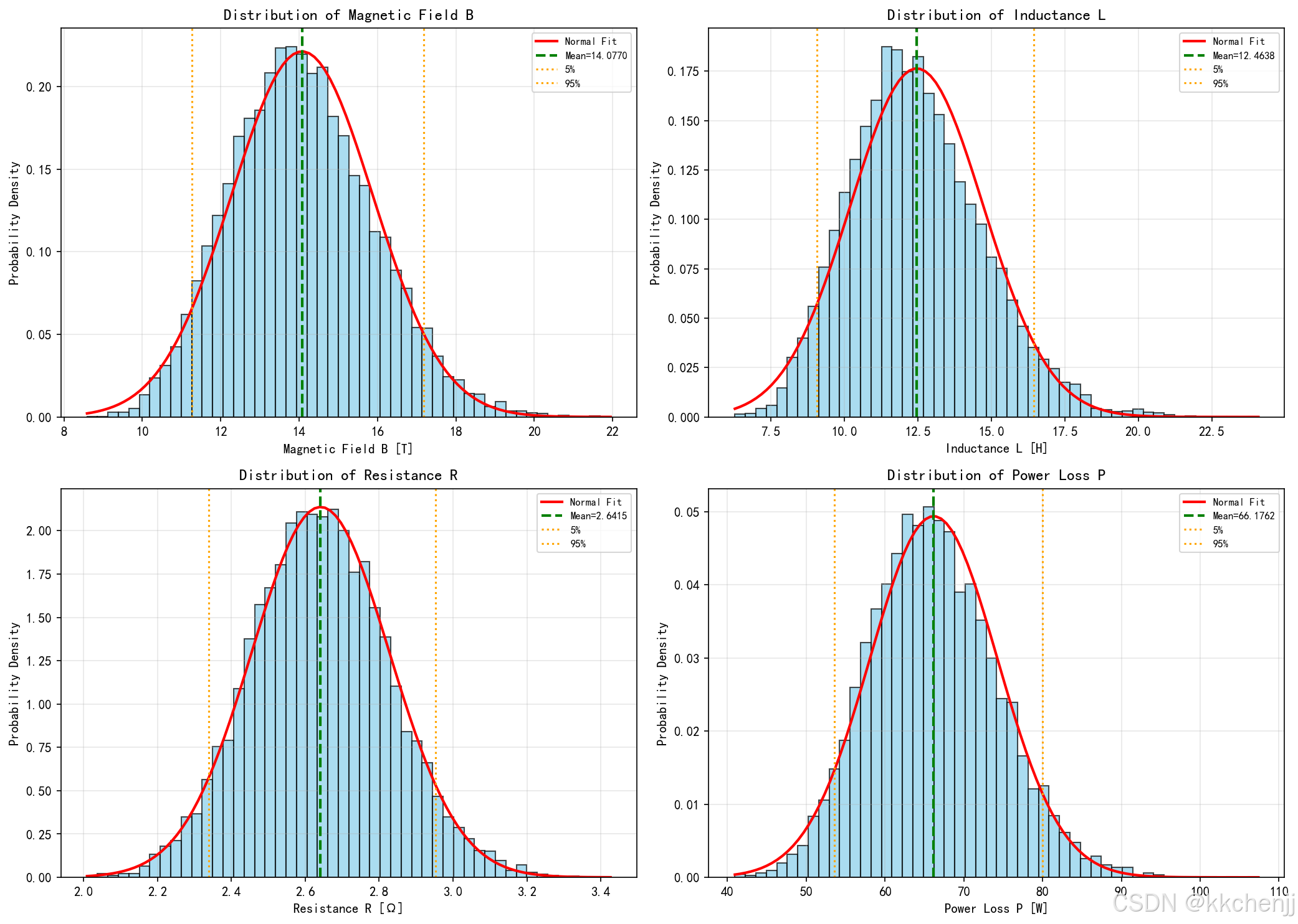
    # 1. 输出分布直方图
    fig, axes = plt.subplots(2, 2, figsize=(14, 10))
    
    outputs = ['B_center', 'L_inductance', 'R_coil', 'P_loss']
    titles = ['Magnetic Field B [T]', 'Inductance L [H]', 
              'Resistance R [Ω]', 'Power Loss P [W]']
    
    for idx, (ax, output, title) in enumerate(zip(axes.flat, outputs, titles)):
        data = results[output]
        
        # 直方图
        ax.hist(data, bins=50, density=True, alpha=0.7, color='skyblue', edgecolor='black')
        
        # 拟合正态分布
        mu, sigma = np.mean(data), np.std(data)
        x = np.linspace(data.min(), data.max(), 100)
        ax.plot(x, stats.norm.pdf(x, mu, sigma), 'r-', linewidth=2, label='Normal Fit')
        
        # 统计信息
        ax.axvline(mu, color='green', linestyle='--', linewidth=2, label=f'Mean={mu:.4f}')
        ax.axvline(np.percentile(data, 5), color='orange', linestyle=':', label='5%')
        ax.axvline(np.percentile(data, 95), color='orange', linestyle=':', label='95%')
        
        ax.set_xlabel(title)
        ax.set_ylabel('Probability Density')
        ax.set_title(f'Distribution of {title.split("[")[0].strip()}')
        ax.legend(fontsize=8)
        ax.grid(True, alpha=0.3)
    
    plt.tight_layout()
    plt.savefig('fig1_output_distributions.png', dpi=150, bbox_inches='tight')
    print("  fig1_output_distributions.png 已保存")
    plt.close()
    
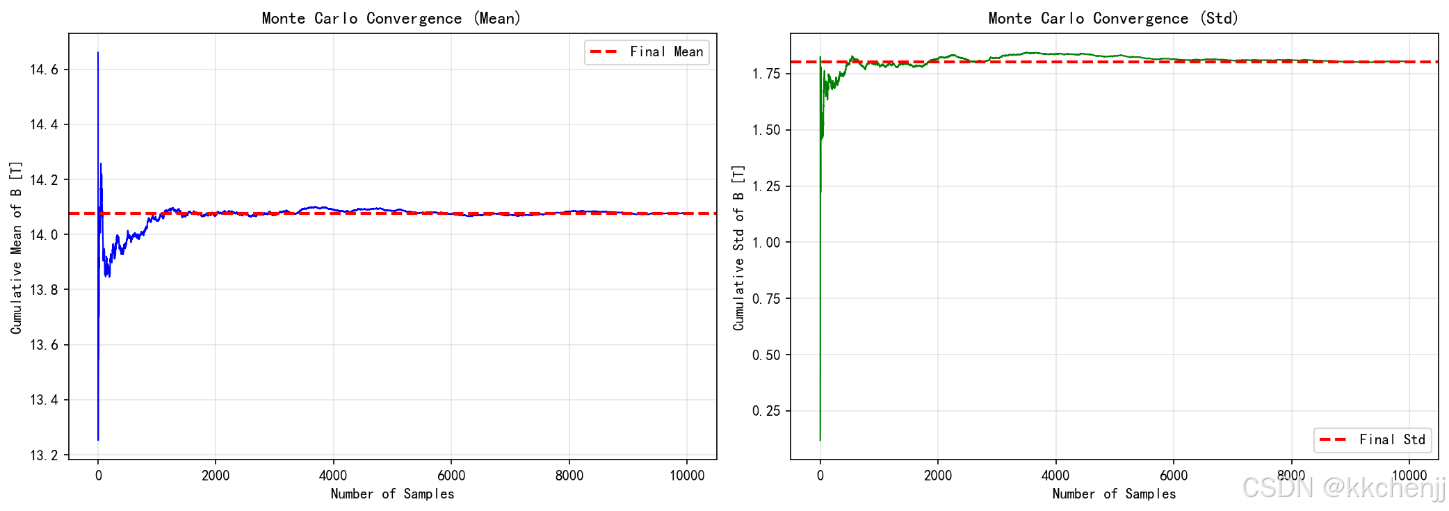
    # 2. 收敛性分析
    fig, axes = plt.subplots(1, 2, figsize=(14, 5))
    
    # 均值收敛
    ax = axes[0]
    B_data = results['B_center']
    cumulative_mean = np.cumsum(B_data) / np.arange(1, len(B_data) + 1)
    
    ax.plot(range(1, len(cumulative_mean) + 1), cumulative_mean, 'b-', linewidth=1)
    ax.axhline(np.mean(B_data), color='r', linestyle='--', linewidth=2, label='Final Mean')
    ax.set_xlabel('Number of Samples')
    ax.set_ylabel('Cumulative Mean of B [T]')
    ax.set_title('Monte Carlo Convergence (Mean)')
    ax.legend()
    ax.grid(True, alpha=0.3)
    
    # 标准差收敛
    ax = axes[1]
    cumulative_std = [np.std(B_data[:i]) for i in range(2, len(B_data) + 1)]
    
    ax.plot(range(2, len(cumulative_std) + 2), cumulative_std, 'g-', linewidth=1)
    ax.axhline(np.std(B_data), color='r', linestyle='--', linewidth=2, label='Final Std')
    ax.set_xlabel('Number of Samples')
    ax.set_ylabel('Cumulative Std of B [T]')
    ax.set_title('Monte Carlo Convergence (Std)')
    ax.legend()
    ax.grid(True, alpha=0.3)
    
    plt.tight_layout()
    plt.savefig('fig2_convergence.png', dpi=150, bbox_inches='tight')
    print("  fig2_convergence.png 已保存")
    plt.close()
    
    # 3. 灵敏度分析结果
    fig, axes = plt.subplots(1, 2, figsize=(14, 6))
    
    # Morris筛选结果
    ax = axes[0]
    morris_results = sensitivity.morris_screening(n_trajectories=20)
    
    param_names = list(morris_results.keys())
    mu_stars = [morris_results[p]['mu_star'] for p in param_names]
    sigmas = [morris_results[p]['sigma'] for p in param_names]
    
    x_pos = np.arange(len(param_names))
    ax.bar(x_pos, mu_stars, yerr=sigmas, capsize=5, color='coral', alpha=0.7)
    ax.set_xticks(x_pos)
    ax.set_xticklabels(param_names)
    ax.set_ylabel('Mean Absolute Elementary Effect')
    ax.set_title('Morris Screening Results')
    ax.grid(True, alpha=0.3, axis='y')
    
    # 龙卷风图（局部灵敏度）
    ax = axes[1]
    base_params = {'N': 500, 'I': 5.0, 'L': 0.2, 'R': 0.05, 'mu_r': 1000}
    local_sens = sensitivity.local_sensitivity(base_params)
    
    # 对B_center的灵敏度
    sens_B = [abs(local_sens[p]['B_center']) for p in param_names]
    
    # 排序
    sorted_indices = np.argsort(sens_B)
    sorted_params = [param_names[i] for i in sorted_indices]
    sorted_sens = [sens_B[i] for i in sorted_indices]
    
    colors = ['red' if s > 0.5 else 'orange' if s > 0.2 else 'green' for s in sorted_sens]
    ax.barh(sorted_params, sorted_sens, color=colors, alpha=0.7)
    ax.set_xlabel('Sensitivity Index')
    ax.set_title('Local Sensitivity Analysis (B_center)')
    ax.grid(True, alpha=0.3, axis='x')
    
    plt.tight_layout()
    plt.savefig('fig3_sensitivity.png', dpi=150, bbox_inches='tight')
    print("  fig3_sensitivity.png 已保存")
    plt.close()
    
    # 4. 可靠性分析
    fig, axes = plt.subplots(1, 2, figsize=(14, 6))
    
    # 极限状态函数可视化
    ax = axes[0]
    B_data = results['B_center']
    limit_B = 0.08  # 磁场上限
    
    # 散点图
    safe = B_data <= limit_B
    failed = B_data > limit_B
    
    ax.scatter(np.where(safe)[0], B_data[safe], c='green', alpha=0.5, s=10, label='Safe')
    ax.scatter(np.where(failed)[0], B_data[failed], c='red', alpha=0.5, s=10, label='Failed')
    ax.axhline(limit_B, color='black', linestyle='--', linewidth=2, label=f'Limit = {limit_B} T')
    
    ax.set_xlabel('Sample Index')
    ax.set_ylabel('B [T]')
    ax.set_title('Limit State Visualization')
    ax.legend()
    ax.grid(True, alpha=0.3)
    
    # 累积分布函数
    ax = axes[1]
    sorted_B = np.sort(B_data)
    cdf = np.arange(1, len(sorted_B) + 1) / len(sorted_B)
    
    ax.plot(sorted_B, cdf, 'b-', linewidth=2)
    ax.axvline(limit_B, color='red', linestyle='--', linewidth=2, label=f'Limit = {limit_B} T')
    ax.axhline(np.mean(B_data <= limit_B), color='green', linestyle=':', 
              label=f'Reliability = {np.mean(B_data <= limit_B):.4f}')
    
    ax.set_xlabel('B [T]')
    ax.set_ylabel('Cumulative Probability')
    ax.set_title('Cumulative Distribution Function')
    ax.legend()
    ax.grid(True, alpha=0.3)
    
    plt.tight_layout()
    plt.savefig('fig4_reliability.png', dpi=150, bbox_inches='tight')
    print("  fig4_reliability.png 已保存")
    plt.close()


# ============================================================
# 第七部分：主程序
# ============================================================

if __name__ == "__main__":
    print("="*70)
    print("主题033: 电磁场仿真不确定性量化")
    print("不确定性量化在电磁场仿真中的应用")
    print("="*70)
    
    # 1. 定义模型
    print("\n[1/5] 定义电磁模型与不确定性...")
    model = ElectromagneticModel()
    print("  输入参数不确定性:")
    for name, unc in model.uncertainties.items():
        print(f"    {name}: {unc.distribution}, μ={unc.mean}, σ={unc.std}")
    
    # 2. 蒙特卡洛模拟
    print("\n[2/5] 执行蒙特卡洛模拟...")
    mc_sim = MonteCarloSimulation(model, n_samples=10000)
    statistics = mc_sim.run()
    
    print("\n  输出统计量:")
    for output_name, output_stats in statistics.items():
        print(f"    {output_name}:")
        print(f"      均值: {output_stats['mean']:.6e}")
        print(f"      标准差: {output_stats['std']:.6e}")
        print(f"      变异系数: {output_stats['cv']:.4f}")
        print(f"      95%置信区间: [{output_stats['q05']:.6e}, {output_stats['q95']:.6e}]")
    
    # 3. 多项式混沌展开
    print("\n[3/5] 构建多项式混沌展开模型...")
    # 准备训练数据
    n_pce_samples = 500
    input_samples = model.sample_inputs(n_pce_samples)
    
    # 标准化输入
    xi = np.zeros((n_pce_samples, 5))
    for i, sample in enumerate(input_samples):
        xi[i, 0] = (sample['N'] - 500) / 25
        xi[i, 1] = (sample['I'] - 5.0) / 0.25
        xi[i, 2] = (sample['L'] - 0.2) / 0.02
        xi[i, 3] = (sample['R'] - 0.05) / 0.0025
        xi[i, 4] = (sample['mu_r'] - 1000) / 100
    
    # 输出
    y_B = np.array([model.evaluate(s)['B_center'] for s in input_samples])
    
    # 拟合PCE
    pce = PolynomialChaosExpansion(order=3)
    pce.fit(xi, y_B)
    
    pce_stats = pce.compute_statistics()
    print(f"\n  PCE统计量:")
    print(f"    均值: {pce_stats['mean']:.6e}")
    print(f"    标准差: {pce_stats['std']:.6e}")
    
    # 4. 灵敏度分析
    print("\n[4/5] 执行灵敏度分析...")
    sensitivity = SensitivityAnalysis(model)
    
    # Morris筛选
    print("\n  Morris筛选结果:")
    morris_results = sensitivity.morris_screening(n_trajectories=20)
    for param_name in ['N', 'I', 'L', 'R', 'mu_r']:
        result = morris_results[param_name]
        print(f"    {param_name}: μ*={result['mu_star']:.4f}, σ={result['sigma']:.4f}")
    
    # 局部灵敏度
    print("\n  局部灵敏度分析 (基准点):")
    base_params = {'N': 500, 'I': 5.0, 'L': 0.2, 'R': 0.05, 'mu_r': 1000}
    local_sens = sensitivity.local_sensitivity(base_params)
    for param_name in ['N', 'I', 'L', 'R', 'mu_r']:
        print(f"    {param_name}对B_center的灵敏度: {local_sens[param_name]['B_center']:.4f}")
    
    # 5. 可靠性分析
    print("\n[5/5] 执行可靠性分析...")
    reliability = ReliabilityAnalysis(mc_sim)
    
    # 定义极限状态：B_center <= 0.08 T
    def limit_state_B(results, idx):
        return results['B_center'][idx] > 0.08
    
    rel_results = reliability.compute_reliability(limit_state_B, target_probability=0.95)
    
    print(f"\n  可靠性分析结果:")
    print(f"    失效概率 Pf: {rel_results['failure_probability']:.6f}")
    print(f"    可靠度: {rel_results['reliability']:.6f}")
    print(f"    可靠性指数 β: {rel_results['reliability_index']:.4f}")
    print(f"    Pf 95%置信区间: [{rel_results['pf_ci_lower']:.6f}, {rel_results['pf_ci_upper']:.6f}]")
    print(f"    是否满足目标可靠度(0.95): {rel_results['target_met']}")
    
    # 6. 生成可视化
    print("\n[6/6] 生成可视化...")
    create_visualizations(mc_sim, pce, sensitivity, reliability)
    
    # 保存结果
    output_results = {
        'monte_carlo': {
            'n_samples': mc_sim.n_samples,
            'statistics': statistics
        },
        'pce': {
            'order': pce.order,
            'r2': float(pce.r2),
            'mean': float(pce_stats['mean']),
            'std': float(pce_stats['std'])
        },
        'sensitivity': {
            'morris': morris_results,
            'local': {k: v['B_center'] for k, v in local_sens.items()}
        },
        'reliability': rel_results
    }
    
    with open('uncertainty_results.json', 'w', encoding='utf-8') as f:
        json.dump(output_results, f, indent=2, ensure_ascii=False)
    
    print("\n" + "="*70)
    print("主题033仿真完成！")
    print("="*70)
    print("\n生成的文件:")
    print("  - fig1_output_distributions.png: 输出分布直方图")
    print("  - fig2_convergence.png: 蒙特卡洛收敛性")
    print("  - fig3_sensitivity.png: 灵敏度分析")
    print("  - fig4_reliability.png: 可靠性分析")
    print("  - uncertainty_results.json: 不确定性量化结果")
    print("="*70)