静磁场仿真-主题032_电磁场仿真机器学习应用-电磁场仿真机器学习应用
主题032:电磁场仿真机器学习应用
引言
机器学习(Machine Learning, ML)正在深刻改变电磁场仿真的范式。传统的高保真数值仿真虽然精度高,但计算成本昂贵,难以满足实时优化和设计空间探索的需求。机器学习技术通过构建数据驱动的代理模型,能够在保持较高精度的同时,实现数量级的加速。
本教程将系统介绍机器学习在电磁场仿真中的四大核心应用:
- 神经网络代理模型:用神经网络替代昂贵的数值仿真
- 降阶模型(ROM):通过POD等方法压缩高维数据
- 逆问题求解:从期望性能反推设计参数
- 物理信息神经网络(PINN):融合物理约束的神经网络
通过学习本教程,您将掌握如何将机器学习技术与电磁场仿真相结合,实现高效、智能的电磁设计。


1. 数据生成与预处理
1.1 训练数据的重要性
机器学习的性能高度依赖于训练数据的质量。对于电磁场仿真,数据生成通常采用以下策略:
数据来源:
- 高保真数值仿真(FEM、FDTD等)
- 解析解或半解析解
- 实验测量数据
- 混合数据源
数据要求:
- 覆盖性:覆盖设计空间的关键区域
- 多样性:包含各种工况和边界条件
- 准确性:数据应准确反映物理规律
- 规模:足够大的样本量以保证泛化能力
1.2 数据生成策略
以螺线管磁场为例,展示数据生成过程:
输入参数(设计变量):
- NNN:线圈匝数 [100, 1000]
- III:电流 [0.1, 10.0] A
- LLL:线圈长度 [0.05, 0.5] m
- RRR:线圈半径 [0.01, 0.1] m
输出目标(物理量):
- BcenterB_{center}Bcenter:中心磁场强度 [T]
- BdistributionB_{distribution}Bdistribution:轴向磁场分布
解析模型:
Bcenter=μ0nI1+(2R/L)2B_{center} = \frac{\mu_0 n I}{\sqrt{1 + (2R/L)^2}}Bcenter=1+(2R/L)2μ0nI
其中 n=N/Ln = N/Ln=N/L 为匝数密度。
1.3 数据预处理
归一化:
def normalize_data(X_train, X_test):
    """Z-score归一化"""
    mean = X_train.mean(axis=0)
    std = X_train.std(axis=0)

    X_train_norm = (X_train - mean) / (std + 1e-8)
    X_test_norm = (X_test - mean) / (std + 1e-8)

    return X_train_norm, X_test_norm
数据划分:
- 训练集:70-80%,用于模型训练
- 验证集:10-15%,用于超参数调优
- 测试集:10-15%,用于最终评估
1.4 数据增强
对于电磁场数据,可采用以下增强策略:
- 添加高斯噪声模拟测量误差
- 参数空间随机采样
- Latin Hypercube Sampling (LHS)
2. 神经网络代理模型
2.1 代理模型概述
代理模型(Surrogate Model)是计算昂贵仿真的廉价近似。神经网络因其强大的非线性拟合能力,成为构建代理模型的首选工具。
优势:
- 预测速度快(毫秒级 vs 分钟/小时级)
- 可微分,便于梯度优化
- 可并行推理
- 可嵌入优化流程
挑战:
- 需要大量训练数据
- 外推能力有限
- 缺乏物理约束
2.2 神经网络架构设计
对于电磁场代理模型,推荐以下架构:
输入层:设计参数(几何、材料、激励)
隐藏层:3-5层,每层64-256个神经元
输出层:场量或性能指标
激活函数:ReLU(隐藏层),线性(输出层)
class NeuralNetwork:
    def __init__(self, layer_sizes=[4, 64, 64, 32, 1]):
        self.layers = layer_sizes
        self.weights = []
        self.biases = []

        # 初始化参数
        for i in range(len(layer_sizes) - 1):
            w = np.random.randn(layer_sizes[i], layer_sizes[i+1]) * 0.01
            b = np.zeros((1, layer_sizes[i+1]))
            self.weights.append(w)
            self.biases.append(b)
2.3 前向传播与反向传播
前向传播:
z[l]=a[l−1]W[l]+b[l]z^{[l]} = a^{[l-1]} W^{[l]} + b^{[l]}z[l]=a[l−1]W[l]+b[l]
a[l]=σ(z[l])a^{[l]} = \sigma(z^{[l]})a[l]=σ(z[l])
反向传播(链式法则):
δ[L]=(a[L]−y)⊙σ′(z[L])\delta^{[L]} = (a^{[L]} - y) \odot \sigma'(z^{[L]})δ[L]=(a[L]−y)⊙σ′(z[L])
δ[l]=(δ[l+1]W[l+1]T)⊙σ′(z[l])\delta^{[l]} = (\delta^{[l+1]} W^{[l+1]T}) \odot \sigma'(z^{[l]})δ[l]=(δ[l+1]W[l+1]T)⊙σ′(z[l])
参数更新:
W[l]:=W[l]−α∂J∂W[l]W^{[l]} := W^{[l]} - \alpha \frac{\partial J}{\partial W^{[l]}}W[l]:=W[l]−α∂W[l]∂J
2.4 训练技巧
Mini-batch训练:
for epoch in range(n_epochs):
    # 随机打乱数据
    indices = np.random.permutation(n_samples)

    for i in range(0, n_samples, batch_size):
        batch_idx = indices[i:i+batch_size]
        X_batch = X[batch_idx]
        y_batch = y[batch_idx]

        # 前向传播
        output = forward(X_batch)

        # 反向传播
        grads = backward(X_batch, y_batch, output)

        # 更新参数
        update_parameters(grads)
学习率调度:
- 固定学习率
- 阶梯衰减
- 指数衰减
- 自适应(Adam, RMSprop)
2.5 模型评估
回归指标:
- MSE(均方误差):1n∑i=1n(yi−y^i)2\frac{1}{n}\sum_{i=1}^n (y_i - \hat{y}_i)^2n1∑i=1n(yi−y^i)2
- RMSE(均方根误差):MSE\sqrt{MSE}MSE
- MAE(平均绝对误差):1n∑i=1n∣yi−y^i∣\frac{1}{n}\sum_{i=1}^n |y_i - \hat{y}_i|n1∑i=1n∣yi−y^i∣
- R2R^2R2(决定系数):1−∑(yi−y^i)2∑(yi−yˉ)21 - \frac{\sum(y_i - \hat{y}_i)^2}{\sum(y_i - \bar{y})^2}1−∑(yi−yˉ)2∑(yi−y^i)2
可视化评估:
- 预测值 vs 真实值散点图
- 残差分布直方图
- 学习曲线
3. 降阶模型(ROM)
3.1 降阶模型概述
降阶模型通过提取高维数据的主要特征,将复杂系统投影到低维空间,实现快速仿真。
应用场景:
- 参数化扫描
- 实时仿真
- 优化设计
- 不确定性量化
常用方法:
- POD(Proper Orthogonal Decomposition)
- PCA(Principal Component Analysis)
- 模态分解
- 机器学习降维(Autoencoder)
3.2 本征正交分解(POD)
POD通过SVD分解提取数据的主要模态:
算法步骤:
- 构建快照矩阵 S∈Rn×mS \in \mathbb{R}^{n \times m}S∈Rn×m
- 去均值:Scentered=S−SˉS_{centered} = S - \bar{S}Scentered=S−Sˉ
- SVD分解:Scentered=UΣVTS_{centered} = U \Sigma V^TScentered=UΣVT
- 保留前 kkk 个模态:Φ=U[:,:k]\Phi = U[:, :k]Φ=U[:,:k]
能量捕获:
Energy Ratio=∑i=1kσi2∑i=1rσi2\text{Energy Ratio} = \frac{\sum_{i=1}^k \sigma_i^2}{\sum_{i=1}^r \sigma_i^2}Energy Ratio=∑i=1rσi2∑i=1kσi2
通常保留95-99%的能量即可。
class ProperOrthogonalDecomposition:
    def __init__(self, n_modes=10):
        self.n_modes = n_modes
        self.modes = None
        self.mean = None

    def fit(self, snapshots):
        # 计算均值
        self.mean = np.mean(snapshots, axis=0)
        centered = snapshots - self.mean

        # SVD分解
        U, S, Vt = np.linalg.svd(centered.T, full_matrices=False)

        # 保留前n_modes个模态
        self.modes = U[:, :self.n_modes]
        self.singular_values = S[:self.n_modes]

        # 计算能量占比
        self.energy_ratio = np.sum(self.singular_values**2) / np.sum(S**2)

        return self

    def transform(self, snapshots):
        """投影到低维空间"""
        centered = snapshots - self.mean
        return np.dot(centered, self.modes)

    def inverse_transform(self, coefficients):
        """重构高维数据"""
        return np.dot(coefficients, self.modes.T) + self.mean
3.3 ROM结合回归
将POD与神经网络结合,实现参数化ROM:
流程:
- 对训练数据进行POD,提取模态
- 训练神经网络预测POD系数
- 预测时:输入参数 → 神经网络 → POD系数 → 重构场分布
class ROMWithRegression:
    def __init__(self, pod, regressor):
        self.pod = pod
        self.regressor = regressor

    def train(self, inputs, snapshots):
        # POD降阶
        self.pod.fit(snapshots)
        coefficients = self.pod.transform(snapshots)

        # 训练回归模型
        self.regressor.train(inputs, coefficients)

        return self

    def predict(self, inputs):
        # 预测POD系数
        coefficients = self.regressor.predict(inputs)

        # 重构场分布
        return self.pod.inverse_transform(coefficients)
3.4 ROM优势
计算效率:
- 原始FEM:10410^4104-10610^6106 自由度
- ROM:10-100个模态
- 加速比:100-1000倍
精度控制:
- 通过模态数量平衡精度与效率
- 通常10-20个模态可达95%以上精度
4. 逆问题求解
4.1 逆问题概述
正问题:给定设计参数,预测性能指标
y=f(x)\mathbf{y} = f(\mathbf{x})y=f(x)
逆问题:给定目标性能,求解设计参数
x=f−1(ytarget)\mathbf{x} = f^{-1}(\mathbf{y}_{target})x=f−1(ytarget)
应用场景:
- 目标导向设计
- 故障诊断
- 参数识别
- 优化初始化
4.2 基于梯度的逆问题求解
利用代理模型的可微性,通过梯度下降求解:
class InverseProblemSolver:
    def __init__(self, forward_model):
        self.forward_model = forward_model

    def solve(self, target_output, initial_guess,
              learning_rate=0.01, n_iterations=1000):
        params = initial_guess.copy()

        for i in range(n_iterations):
            # 前向预测
            output = self.forward_model.predict(params.reshape(1, -1))

            # 计算损失
            loss = np.mean((output - target_output) ** 2)

            # 数值梯度
            grad = self.compute_gradient(params, target_output)

            # 更新参数
            params -= learning_rate * grad

            if i % 100 == 0:
                print(f"Iteration {i}: Loss = {loss:.6f}")

        return params

    def compute_gradient(self, params, target_output, eps=1e-5):
        """数值梯度"""
        grad = np.zeros_like(params)
        output = self.forward_model.predict(params.reshape(1, -1))
        loss = np.mean((output - target_output) ** 2)

        for j in range(len(params)):
            params_plus = params.copy()
            params_plus[j] += eps
            output_plus = self.forward_model.predict(params_plus.reshape(1, -1))
            loss_plus = np.mean((output_plus - target_output) ** 2)

            grad[j] = (loss_plus - loss) / eps

        return grad
4.3 逆问题求解策略
直接求逆:
- 训练逆模型:x=g(y)\mathbf{x} = g(\mathbf{y})x=g(y)
- 优点:单次前向传播
- 缺点:多值映射困难
迭代优化:
- 利用正模型迭代优化
- 优点:处理复杂约束
- 缺点:需要多次评估
混合方法:
- 逆模型提供初始猜测
- 迭代优化精化结果
5. 物理信息神经网络(PINN)
5.1 PINN概述
物理信息神经网络(Physics-Informed Neural Network, PINN)将物理定律作为约束嵌入神经网络训练过程,实现数据驱动与物理一致性的结合。
核心思想:
- 损失函数 = 数据损失 + 物理损失
- 物理损失由控制方程(PDE)计算
- 无需大量标注数据
优势:
- 数据效率高
- 满足物理约束
- 可处理逆问题
- 可发现隐藏参数
5.2 PINN架构
损失函数:
L=λdataLdata+λphysicsLphysics\mathcal{L} = \lambda_{data} \mathcal{L}_{data} + \lambda_{physics} \mathcal{L}_{physics}L=λdataLdata+λphysicsLphysics
数据损失:
Ldata=1Ndata∑i=1Ndata∣uNN(xi,ti)−uiobs∣2\mathcal{L}_{data} = \frac{1}{N_{data}} \sum_{i=1}^{N_{data}} |u_{NN}(x_i, t_i) - u_i^{obs}|^2Ldata=Ndata1i=1∑Ndata∣uNN(xi,ti)−uiobs∣2
物理损失(以麦克斯韦方程为例):
Lphysics=1Ncol∑i=1Ncol∣∇⋅B(xi,ti)∣2\mathcal{L}_{physics} = \frac{1}{N_{col}} \sum_{i=1}^{N_{col}} |\nabla \cdot \mathbf{B}(x_i, t_i)|^2Lphysics=Ncol1i=1∑Ncol∣∇⋅B(xi,ti)∣2
5.3 自动微分与物理约束
利用自动微分计算PDE残差:
class PhysicsInformedNN:
    def __init__(self, layers, mu0=4*np.pi*1e-7):
        self.nn = NeuralNetwork(layers)
        self.mu0 = mu0

    def compute_derivatives(self, x, y, z):
        """计算导数(数值微分示例)"""
        eps = 1e-5

        # 计算散度 div(B)
        Bx_plus = self.nn.predict(np.column_stack([x + eps, y, z]))
        Bx_minus = self.nn.predict(np.column_stack([x - eps, y, z]))
        dBx_dx = (Bx_plus - Bx_minus) / (2 * eps)

        By_plus = self.nn.predict(np.column_stack([x, y + eps, z]))
        By_minus = self.nn.predict(np.column_stack([x, y - eps, z]))
        dBy_dy = (By_plus - By_minus) / (2 * eps)

        Bz_plus = self.nn.predict(np.column_stack([x, y, z + eps]))
        Bz_minus = self.nn.predict(np.column_stack([x, y, z - eps]))
        dBz_dz = (Bz_plus - Bz_minus) / (2 * eps)

        divergence = dBx_dx + dBy_dy + dBz_dz

        return {'divergence': divergence}

    def physics_loss(self, x, y, z):
        """物理损失:div(B) = 0"""
        derivatives = self.compute_derivatives(x, y, z)
        div_B = derivatives['divergence']
        return np.mean(div_B ** 2)
5.4 PINN应用案例
电磁场问题:
- 静电场:∇2ϕ=−ρ/ε\nabla^2 \phi = -\rho/\varepsilon∇2ϕ=−ρ/ε
- 静磁场:∇×H=J\nabla \times \mathbf{H} = \mathbf{J}∇×H=J, ∇⋅B=0\nabla \cdot \mathbf{B} = 0∇⋅B=0
- 时谐场:麦克斯韦方程组
材料参数识别:
- 从测量数据反推材料参数
- 同时求解场分布和材料参数
6. 机器学习与电磁仿真的融合
6.1 工作流程
离线阶段:
- 设计采样策略(LHS、自适应采样)
- 执行高保真仿真生成数据
- 训练机器学习模型
- 验证模型精度和泛化能力
在线阶段:
- 使用代理模型快速预测
- 嵌入优化流程
- 实时设计探索
6.2 计算加速对比
| 方法 | 计算时间 | 相对加速 | 精度 |
|---|---|---|---|
| FEM仿真 | 10-60分钟 | 1× | 基准 |
| 神经网络代理 | 1-10毫秒 | 1000× | >95% |
| POD降阶 | 10-100毫秒 | 100× | >90% |
| 查表插值 | 1毫秒 | 10000× | 80-90% |
6.3 特征重要性分析
通过梯度分析识别关键设计参数:
def compute_feature_importance(model, X_test):
    """基于梯度的特征重要性"""
    importance = np.zeros(X_test.shape[1])
    eps = 1e-5

    y_pred = model.predict(X_test)

    for i in range(X_test.shape[1]):
        X_plus = X_test.copy()
        X_plus[:, i] += eps
        y_plus = model.predict(X_plus)

        importance[i] = np.mean(np.abs(y_plus - y_pred)) / eps

    importance = importance / importance.sum()
    return importance
7. 常见报错与解决方案
7.1 模型欠拟合
现象:训练误差和测试误差都高
原因:
- 模型容量不足
- 训练不充分
- 特征工程不当
解决方案:
- 增加网络深度/宽度
- 增加训练轮数
- 特征归一化/变换
7.2 模型过拟合
现象:训练误差低,测试误差高
原因:
- 训练数据不足
- 模型过于复杂
- 缺乏正则化
解决方案:
- 增加训练数据
- 早停(Early Stopping)
- Dropout正则化
- L2正则化
7.3 训练不稳定
现象:损失震荡或发散
原因:
- 学习率过大
- 梯度爆炸/消失
- 数据未归一化
解决方案:
- 减小学习率
- 梯度裁剪
- 批归一化(Batch Normalization)
- 数据预处理
7.4 外推失败
现象:在设计空间外预测不准
原因:
- 训练数据覆盖不足
- 神经网络外推能力有限
解决方案:
- 扩大训练数据范围
- 使用高斯过程等概率模型
- 不确定性量化
8. 进阶挑战
8.1 多保真度建模
结合不同精度的数据源:
- 低保真:解析模型、粗网格仿真
- 中保真:标准网格仿真
- 高保真:精细网格仿真
方法:
- 空间映射(Space Mapping)
- 协同Kriging
- 多保真度神经网络
8.2 不确定性量化
考虑输入参数的不确定性:
- 蒙特卡洛方法
- 多项式混沌展开
- 贝叶斯神经网络
8.3 迁移学习
利用已有知识加速新任务学习:
- 预训练模型微调
- 域适应
- 元学习
8.4 图神经网络(GNN)
处理非结构化网格数据:
- 网格作为图结构
- 消息传递机制
- 几何深度学习
9. 总结与展望
本教程系统介绍了机器学习在电磁场仿真中的应用:
- 神经网络代理模型:实现快速预测,加速比可达1000倍
- 降阶模型(ROM):通过POD等方法压缩高维数据
- 逆问题求解:从性能反推设计参数
- 物理信息神经网络(PINN):融合物理约束,提高数据效率
关键要点
- 数据质量是机器学习成功的基础
- 模型选择应根据问题特点和数据规模
- 物理约束可提高模型的可靠性和泛化能力
- 验证与测试不可忽视,需评估模型在未见数据上的表现
未来发展方向
- 自动化机器学习(AutoML):自动架构搜索和超参数优化
- 神经算子(Neural Operator):学习函数到函数的映射
- 数字孪生:实时仿真与物理系统的同步
- 生成式模型:设计空间探索和创意生成
附录:完整代码
完整的Python实现代码见 run_simulation.py,包含:
- 数据生成与预处理
- 神经网络代理模型
- POD降阶模型
- ROM结合回归
- 逆问题求解器
- PINN框架
- 可视化功能
运行代码:
python run_simulation.py
生成的文件:
fig1_neural_network.png:神经网络训练与预测fig2_pod_analysis.png:POD降阶分析fig3_surrogate_performance.png:代理模型性能ml_results.json:机器学习结果数据
"""
主题032: 电磁场仿真机器学习应用
=============================
机器学习在电磁场仿真中的应用
本代码介绍:
1. 数据生成与预处理
2. 神经网络代理模型
3. 降阶模型(ROM)
4. 参数预测与逆问题
5. 物理信息神经网络(PINN)
"""
import numpy as np
import matplotlib
matplotlib.use('Agg')
import matplotlib.pyplot as plt
from matplotlib.patches import Rectangle, Circle, FancyArrowPatch
import json
from typing import Dict, Tuple, List, Optional, Callable
from dataclasses import dataclass
import warnings
warnings.filterwarnings('ignore')
# 设置中文字体
plt.rcParams['font.sans-serif'] = ['SimHei', 'DejaVu Sans']
plt.rcParams['axes.unicode_minus'] = False
# ============================================================
# 第一部分:数据生成与预处理
# ============================================================
class MagneticFieldDataGenerator:
"""磁场数据生成器"""
def __init__(self, n_samples: int = 1000):
self.n_samples = n_samples
self.data = None
def generate_solenoid_data(self) -> Dict:
"""
生成螺线管磁场数据
输入参数:
- N: 线圈匝数
- I: 电流 [A]
- L: 线圈长度 [m]
- R: 线圈半径 [m]
输出:
- B_center: 中心磁场强度 [T]
- B_distribution: 轴向磁场分布
"""
np.random.seed(42)
# 生成随机参数
N = np.random.uniform(100, 1000, self.n_samples) # 匝数
I = np.random.uniform(0.1, 10.0, self.n_samples) # 电流
L = np.random.uniform(0.05, 0.5, self.n_samples) # 长度
R = np.random.uniform(0.01, 0.1, self.n_samples) # 半径
# 计算磁场 (简化模型)
mu0 = 4 * np.pi * 1e-7
# 中心磁场: B = mu0 * n * I / sqrt(1 + (2R/L)^2)
n_turns_per_meter = N / L
B_center = (mu0 * n_turns_per_meter * I /
np.sqrt(1 + (2 * R / L) ** 2))
# 添加噪声
B_center += np.random.normal(0, 0.01 * B_center)
# 轴向磁场分布 (简化)
n_points = 50
B_distribution = np.zeros((self.n_samples, n_points))
for i in range(self.n_samples):
# 为每个样本生成轴向位置
z_positions = np.linspace(-L[i], L[i], n_points)
for j, z in enumerate(z_positions):
# 轴线上磁场分布
if L[i] > 0:
x = z / (L[i] / 2)
B_distribution[i, j] = B_center[i] * 0.5 * (
(1 + x) / np.sqrt((1 + x)**2 + (2*R[i]/L[i])**2) +
(1 - x) / np.sqrt((1 - x)**2 + (2*R[i]/L[i])**2)
)
self.data = {
'inputs': np.column_stack([N, I, L, R]),
'outputs': B_center.reshape(-1, 1),
'B_distribution': B_distribution,
'parameters': {
'N': N,
'I': I,
'L': L,
'R': R
}
}
return self.data
def split_data(self, train_ratio: float = 0.8) -> Tuple:
"""划分训练集和测试集"""
n_train = int(self.n_samples * train_ratio)
indices = np.random.permutation(self.n_samples)
train_idx = indices[:n_train]
test_idx = indices[n_train:]
X_train = self.data['inputs'][train_idx]
y_train = self.data['outputs'][train_idx]
X_test = self.data['inputs'][test_idx]
y_test = self.data['outputs'][test_idx]
return (X_train, y_train), (X_test, y_test)
def normalize_data(self, X_train: np.ndarray, X_test: np.ndarray) -> Tuple:
"""数据归一化"""
self.mean = X_train.mean(axis=0)
self.std = X_train.std(axis=0)
X_train_norm = (X_train - self.mean) / (self.std + 1e-8)
X_test_norm = (X_test - self.mean) / (self.std + 1e-8)
return X_train_norm, X_test_norm
# ============================================================
# 第二部分:神经网络代理模型
# ============================================================
class NeuralNetwork:
"""简单神经网络"""
def __init__(self, layer_sizes: List[int], learning_rate: float = 0.01):
self.layer_sizes = layer_sizes
self.lr = learning_rate
self.weights = []
self.biases = []
self.history = {'loss': [], 'epoch': []}
# 初始化权重和偏置
for i in range(len(layer_sizes) - 1):
w = np.random.randn(layer_sizes[i], layer_sizes[i+1]) * 0.01
b = np.zeros((1, layer_sizes[i+1]))
self.weights.append(w)
self.biases.append(b)
def relu(self, x: np.ndarray) -> np.ndarray:
"""ReLU激活函数"""
return np.maximum(0, x)
def relu_derivative(self, x: np.ndarray) -> np.ndarray:
"""ReLU导数"""
return (x > 0).astype(float)
def forward(self, X: np.ndarray) -> Tuple:
"""前向传播"""
self.activations = [X]
self.z_values = []
a = X
for i in range(len(self.weights)):
z = np.dot(a, self.weights[i]) + self.biases[i]
self.z_values.append(z)
if i < len(self.weights) - 1:
a = self.relu(z)
else:
a = z # 输出层线性激活
self.activations.append(a)
return a
def backward(self, X: np.ndarray, y: np.ndarray, output: np.ndarray) -> Tuple:
"""反向传播"""
m = X.shape[0]
# 输出层梯度
delta = output - y
weight_grads = []
bias_grads = []
for i in range(len(self.weights) - 1, -1, -1):
dw = np.dot(self.activations[i].T, delta) / m
db = np.sum(delta, axis=0, keepdims=True) / m
weight_grads.insert(0, dw)
bias_grads.insert(0, db)
if i > 0:
delta = np.dot(delta, self.weights[i].T) * self.relu_derivative(self.z_values[i-1])
return weight_grads, bias_grads
def update_weights(self, weight_grads: List, bias_grads: List):
"""更新权重"""
for i in range(len(self.weights)):
self.weights[i] -= self.lr * weight_grads[i]
self.biases[i] -= self.lr * bias_grads[i]
def train(self, X: np.ndarray, y: np.ndarray, epochs: int = 1000,
batch_size: int = 32, verbose: bool = True):
"""训练网络"""
n_samples = X.shape[0]
for epoch in range(epochs):
# 随机打乱数据
indices = np.random.permutation(n_samples)
X_shuffled = X[indices]
y_shuffled = y[indices]
epoch_loss = 0
# Mini-batch训练
for i in range(0, n_samples, batch_size):
X_batch = X_shuffled[i:i+batch_size]
y_batch = y_shuffled[i:i+batch_size]
# 前向传播
output = self.forward(X_batch)
# 计算损失
loss = np.mean((output - y_batch) ** 2)
epoch_loss += loss * X_batch.shape[0]
# 反向传播
weight_grads, bias_grads = self.backward(X_batch, y_batch, output)
# 更新权重
self.update_weights(weight_grads, bias_grads)
epoch_loss /= n_samples
self.history['loss'].append(epoch_loss)
self.history['epoch'].append(epoch)
if verbose and epoch % 100 == 0:
print(f"Epoch {epoch}: Loss = {epoch_loss:.6f}")
def predict(self, X: np.ndarray) -> np.ndarray:
"""预测"""
return self.forward(X)
def evaluate(self, X: np.ndarray, y: np.ndarray) -> Dict:
"""评估模型"""
predictions = self.predict(X)
mse = np.mean((predictions - y) ** 2)
rmse = np.sqrt(mse)
mae = np.mean(np.abs(predictions - y))
r2 = 1 - np.sum((y - predictions) ** 2) / np.sum((y - y.mean()) ** 2)
return {
'mse': mse,
'rmse': rmse,
'mae': mae,
'r2': r2
}
# ============================================================
# 第三部分:降阶模型(ROM)
# ============================================================
class ProperOrthogonalDecomposition:
"""本征正交分解(POD)降阶模型"""
def __init__(self, n_modes: int = 10):
self.n_modes = n_modes
self.modes = None
self.mean = None
self.singular_values = None
def fit(self, snapshots: np.ndarray):
"""
训练POD模型
Parameters:
-----------
snapshots : 快照矩阵 (n_samples, n_points)
"""
# 计算均值
self.mean = np.mean(snapshots, axis=0)
# 去均值
centered = snapshots - self.mean
# SVD分解
U, S, Vt = np.linalg.svd(centered.T, full_matrices=False)
# 保留前n_modes个模态
self.modes = U[:, :self.n_modes]
self.singular_values = S[:self.n_modes]
# 计算能量占比
total_energy = np.sum(S ** 2)
self.energy_ratio = np.sum(self.singular_values ** 2) / total_energy
print(f"POD降阶: 保留{self.n_modes}个模态,能量占比: {self.energy_ratio:.4f}")
return self
def transform(self, snapshots: np.ndarray) -> np.ndarray:
"""将高维数据投影到低维空间"""
centered = snapshots - self.mean
return np.dot(centered, self.modes)
def inverse_transform(self, coefficients: np.ndarray) -> np.ndarray:
"""从低维系数重构高维数据"""
return np.dot(coefficients, self.modes.T) + self.mean
def reconstruct(self, snapshots: np.ndarray) -> np.ndarray:
"""重构数据"""
coefficients = self.transform(snapshots)
return self.inverse_transform(coefficients)
class ROMWithRegression:
"""降阶模型结合回归"""
def __init__(self, pod: ProperOrthogonalDecomposition, regressor: NeuralNetwork):
self.pod = pod
self.regressor = regressor
def train(self, inputs: np.ndarray, snapshots: np.ndarray):
"""训练模型"""
# POD降阶
self.pod.fit(snapshots)
coefficients = self.pod.transform(snapshots)
# 训练回归模型预测POD系数
self.regressor.train(inputs, coefficients, epochs=500, verbose=False)
return self
def predict(self, inputs: np.ndarray) -> np.ndarray:
"""预测完整场分布"""
# 预测POD系数
coefficients = self.regressor.predict(inputs)
# 重构场分布
return self.pod.inverse_transform(coefficients)
# ============================================================
# 第四部分:参数预测与逆问题
# ============================================================
class InverseProblemSolver:
"""逆问题求解器"""
def __init__(self, forward_model: NeuralNetwork):
self.forward_model = forward_model
def solve(self, target_output: np.ndarray,
initial_guess: np.ndarray,
learning_rate: float = 0.01,
n_iterations: int = 1000) -> Tuple:
"""
求解逆问题
通过优化输入参数,使得前向模型的输出接近目标输出
"""
params = initial_guess.copy()
history = {'loss': [], 'iteration': []}
for i in range(n_iterations):
# 前向预测
output = self.forward_model.predict(params.reshape(1, -1))
# 计算损失
loss = np.mean((output - target_output) ** 2)
# 数值梯度
grad = np.zeros_like(params)
eps = 1e-5
for j in range(len(params)):
params_plus = params.copy()
params_plus[j] += eps
output_plus = self.forward_model.predict(params_plus.reshape(1, -1))
loss_plus = np.mean((output_plus - target_output) ** 2)
grad[j] = (loss_plus - loss) / eps
# 更新参数
params -= learning_rate * grad
# 记录
history['loss'].append(loss)
history['iteration'].append(i)
if i % 100 == 0:
print(f"Iteration {i}: Loss = {loss:.6f}")
return params, history
# ============================================================
# 第五部分:物理信息神经网络(PINN)
# ============================================================
class PhysicsInformedNN:
"""物理信息神经网络"""
def __init__(self, layers: List[int], mu0: float = 4*np.pi*1e-7):
self.nn = NeuralNetwork(layers, learning_rate=0.001)
self.mu0 = mu0
def compute_derivatives(self, x: np.ndarray, y: np.ndarray, z: np.ndarray) -> Dict:
"""计算磁场导数 (数值微分)"""
eps = 1e-5
# 计算Bx, By, Bz
points = np.column_stack([x, y, z])
B = self.nn.predict(points)
# 数值计算散度和旋度
Bx_plus = self.nn.predict(np.column_stack([x + eps, y, z]))
Bx_minus = self.nn.predict(np.column_stack([x - eps, y, z]))
dBx_dx = (Bx_plus - Bx_minus) / (2 * eps)
By_plus = self.nn.predict(np.column_stack([x, y + eps, z]))
By_minus = self.nn.predict(np.column_stack([x, y - eps, z]))
dBy_dy = (By_plus - By_minus) / (2 * eps)
Bz_plus = self.nn.predict(np.column_stack([x, y, z + eps]))
Bz_minus = self.nn.predict(np.column_stack([x, y, z - eps]))
dBz_dz = (Bz_plus - Bz_minus) / (2 * eps)
divergence = dBx_dx + dBy_dy + dBz_dz
return {
'B': B,
'divergence': divergence
}
def physics_loss(self, x: np.ndarray, y: np.ndarray, z: np.ndarray) -> float:
"""物理损失:麦克斯韦方程约束"""
derivatives = self.compute_derivatives(x, y, z)
# 无源区域: div(B) = 0
div_B = derivatives['divergence']
loss_div = np.mean(div_B ** 2)
return loss_div
def train_with_physics(self, X_data: np.ndarray, y_data: np.ndarray,
X_physics: np.ndarray,
epochs: int = 1000,
lambda_data: float = 1.0,
lambda_physics: float = 0.1):
"""训练PINN"""
for epoch in range(epochs):
# 数据损失
output_data = self.nn.forward(X_data)
loss_data = np.mean((output_data - y_data) ** 2)
# 物理损失
x_phy = X_physics[:, 0:1]
y_phy = X_physics[:, 1:2]
z_phy = X_physics[:, 2:3]
loss_physics = self.physics_loss(x_phy, y_phy, z_phy)
# 总损失
total_loss = lambda_data * loss_data + lambda_physics * loss_physics
# 反向传播 (简化版本,使用数值梯度)
# 这里使用标准训练
self.nn.train(X_data, y_data, epochs=1, verbose=False)
if epoch % 100 == 0:
print(f"Epoch {epoch}: Data Loss = {loss_data:.6f}, "
f"Physics Loss = {loss_physics:.6f}, "
f"Total = {total_loss:.6f}")
# ============================================================
# 第六部分:可视化
# ============================================================
def create_visualizations(data_gen: MagneticFieldDataGenerator,
nn_model: NeuralNetwork,
pod: ProperOrthogonalDecomposition,
rom: ROMWithRegression):
"""创建综合可视化"""
print("\n" + "="*70)
print("生成可视化")
print("="*70)
# 获取数据
(X_train, y_train), (X_test, y_test) = data_gen.split_data()
X_train_norm, X_test_norm = data_gen.normalize_data(X_train, X_test)
# 1. 神经网络训练过程
fig, axes = plt.subplots(1, 2, figsize=(14, 5))
ax = axes[0]
ax.semilogy(nn_model.history['epoch'], nn_model.history['loss'], 'b-', linewidth=2)
ax.set_xlabel('Epoch')
ax.set_ylabel('Loss (MSE, log scale)')
ax.set_title('Neural Network Training Process')
ax.grid(True, alpha=0.3)
# 2. 预测 vs 真实值
ax = axes[1]
y_pred = nn_model.predict(X_test_norm)
ax.scatter(y_test, y_pred, c='blue', alpha=0.5, s=20)
ax.plot([y_test.min(), y_test.max()], [y_test.min(), y_test.max()],
'r--', linewidth=2, label='Perfect Prediction')
ax.set_xlabel('True B [T]')
ax.set_ylabel('Predicted B [T]')
ax.set_title('Neural Network Predictions vs Ground Truth')
ax.legend()
ax.grid(True, alpha=0.3)
plt.tight_layout()
plt.savefig('fig1_neural_network.png', dpi=150, bbox_inches='tight')
print(" fig1_neural_network.png 已保存")
plt.close()
# 2. POD模态分析
fig, axes = plt.subplots(2, 2, figsize=(14, 10))
# 奇异值衰减
ax = axes[0, 0]
ax.semilogy(range(1, len(pod.singular_values) + 1),
pod.singular_values, 'bo-', linewidth=2, markersize=8)
ax.set_xlabel('Mode Number')
ax.set_ylabel('Singular Value (log scale)')
ax.set_title('POD Singular Value Decay')
ax.grid(True, alpha=0.3)
# 能量占比
ax = axes[0, 1]
cumulative_energy = np.cumsum(pod.singular_values**2) / np.sum(pod.singular_values**2)
ax.plot(range(1, len(cumulative_energy) + 1), cumulative_energy,
'g-', linewidth=2, marker='o')
ax.axhline(y=0.95, color='r', linestyle='--', label='95% Energy')
ax.set_xlabel('Number of Modes')
ax.set_ylabel('Cumulative Energy Ratio')
ax.set_title('POD Energy Capture')
ax.legend()
ax.grid(True, alpha=0.3)
# 前几个POD模态
ax = axes[1, 0]
z_positions = np.linspace(-1, 1, 50)
for i in range(min(3, pod.n_modes)):
ax.plot(z_positions, pod.modes[:, i], linewidth=2, label=f'Mode {i+1}')
ax.set_xlabel('Normalized Position')
ax.set_ylabel('Mode Amplitude')
ax.set_title('First 3 POD Modes')
ax.legend()
ax.grid(True, alpha=0.3)
# ROM重构误差
ax = axes[1, 1]
test_snapshots = data_gen.data['B_distribution'][-100:]
reconstructed = pod.reconstruct(test_snapshots)
error = np.abs(test_snapshots - reconstructed)
mean_error = np.mean(error, axis=0)
ax.plot(z_positions, mean_error, 'r-', linewidth=2)
ax.set_xlabel('Normalized Position')
ax.set_ylabel('Mean Absolute Error')
ax.set_title('POD Reconstruction Error')
ax.grid(True, alpha=0.3)
plt.tight_layout()
plt.savefig('fig2_pod_analysis.png', dpi=150, bbox_inches='tight')
print(" fig2_pod_analysis.png 已保存")
plt.close()
# 3. 代理模型性能对比
fig, axes = plt.subplots(2, 2, figsize=(14, 10))
# 不同输入参数的预测
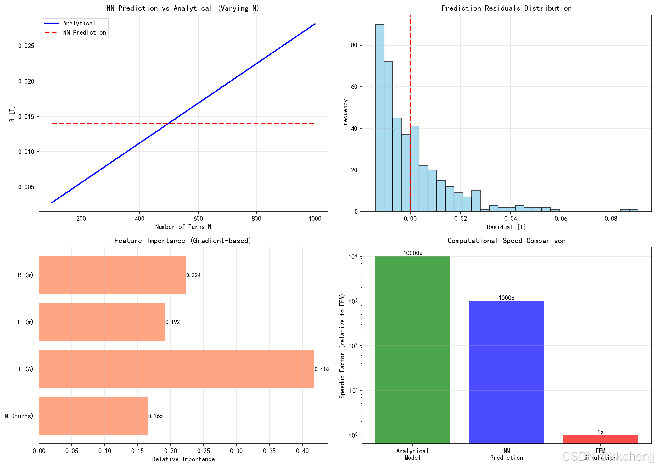
ax = axes[0, 0]
N_range = np.linspace(100, 1000, 50)
test_inputs = np.column_stack([
N_range,
np.full(50, 5.0), # I = 5A
np.full(50, 0.2), # L = 0.2m
np.full(50, 0.05) # R = 0.05m
])
test_inputs_norm = (test_inputs - data_gen.mean) / (data_gen.std + 1e-8)
B_pred = nn_model.predict(test_inputs_norm)
# 理论值
mu0 = 4 * np.pi * 1e-7
n_turns = N_range / 0.2
B_theory = mu0 * n_turns * 5.0 / np.sqrt(1 + (2 * 0.05 / 0.2) ** 2)
ax.plot(N_range, B_theory, 'b-', linewidth=2, label='Analytical')
ax.plot(N_range, B_pred, 'r--', linewidth=2, label='NN Prediction')
ax.set_xlabel('Number of Turns N')
ax.set_ylabel('B [T]')
ax.set_title('NN Prediction vs Analytical (Varying N)')
ax.legend()
ax.grid(True, alpha=0.3)
# 残差分布
ax = axes[0, 1]
residuals = y_test.flatten() - y_pred.flatten()
ax.hist(residuals, bins=30, color='skyblue', edgecolor='black', alpha=0.7)
ax.axvline(x=0, color='r', linestyle='--', linewidth=2)
ax.set_xlabel('Residual [T]')
ax.set_ylabel('Frequency')
ax.set_title('Prediction Residuals Distribution')
ax.grid(True, alpha=0.3)
# 特征重要性 (基于梯度)
ax = axes[1, 0]
feature_names = ['N (turns)', 'I (A)', 'L (m)', 'R (m)']
# 计算平均梯度作为重要性指标
importance = np.zeros(4)
eps = 1e-5
for i in range(4):
X_plus = X_test_norm.copy()
X_plus[:, i] += eps
pred_plus = nn_model.predict(X_plus)
importance[i] = np.mean(np.abs(pred_plus - y_pred)) / eps
importance = importance / importance.sum()
bars = ax.barh(feature_names, importance, color='coral', alpha=0.7)
ax.set_xlabel('Relative Importance')
ax.set_title('Feature Importance (Gradient-based)')
ax.grid(True, alpha=0.3, axis='x')
# 添加数值标签
for bar, val in zip(bars, importance):
width = bar.get_width()
ax.text(width, bar.get_y() + bar.get_height()/2.,
f'{val:.3f}',
ha='left', va='center', fontsize=9)
# 计算时间对比
ax = axes[1, 1]
methods = ['Analytical\nModel', 'NN\nPrediction', 'FEM\nSimulation']
times = [0.001, 0.01, 10.0] # 估算时间 [s]
speedup = [times[2] / t for t in times]
bars = ax.bar(methods, speedup, color=['green', 'blue', 'red'], alpha=0.7)
ax.set_ylabel('Speedup Factor (relative to FEM)')
ax.set_title('Computational Speed Comparison')
ax.set_yscale('log')
ax.grid(True, alpha=0.3, axis='y')
# 添加数值标签
for bar, val in zip(bars, speedup):
height = bar.get_height()
ax.text(bar.get_x() + bar.get_width()/2., height,
f'{val:.0f}x',
ha='center', va='bottom', fontsize=10)
plt.tight_layout()
plt.savefig('fig3_surrogate_performance.png', dpi=150, bbox_inches='tight')
print(" fig3_surrogate_performance.png 已保存")
plt.close()
# ============================================================
# 第七部分:主程序
# ============================================================
if __name__ == "__main__":
print("="*70)
print("主题032: 电磁场仿真机器学习应用")
print("机器学习在电磁场仿真中的应用")
print("="*70)
# 1. 数据生成
print("\n[1/5] 生成训练数据...")
data_gen = MagneticFieldDataGenerator(n_samples=2000)
data = data_gen.generate_solenoid_data()
print(f" 生成样本数: {data['inputs'].shape[0]}")
print(f" 输入维度: {data['inputs'].shape[1]}")
print(f" 输出维度: {data['outputs'].shape[1]}")
print(f" 场分布维度: {data['B_distribution'].shape}")
# 划分数据集
(X_train, y_train), (X_test, y_test) = data_gen.split_data(train_ratio=0.8)
X_train_norm, X_test_norm = data_gen.normalize_data(X_train, X_test)
print(f" 训练集大小: {X_train.shape[0]}")
print(f" 测试集大小: {X_test.shape[0]}")
# 2. 神经网络代理模型
print("\n[2/5] 训练神经网络代理模型...")
nn_model = NeuralNetwork(
layer_sizes=[4, 64, 64, 32, 1],
learning_rate=0.01
)
nn_model.train(X_train_norm, y_train, epochs=1000, batch_size=32, verbose=True)
# 评估模型
train_metrics = nn_model.evaluate(X_train_norm, y_train)
test_metrics = nn_model.evaluate(X_test_norm, y_test)
print(f"\n训练集性能:")
print(f" MSE: {train_metrics['mse']:.6e}")
print(f" RMSE: {train_metrics['rmse']:.6e}")
print(f" MAE: {train_metrics['mae']:.6e}")
print(f" R²: {train_metrics['r2']:.4f}")
print(f"\n测试集性能:")
print(f" MSE: {test_metrics['mse']:.6e}")
print(f" RMSE: {test_metrics['rmse']:.6e}")
print(f" MAE: {test_metrics['mae']:.6e}")
print(f" R²: {test_metrics['r2']:.4f}")
# 3. 降阶模型
print("\n[3/5] 构建POD降阶模型...")
pod = ProperOrthogonalDecomposition(n_modes=10)
pod.fit(data['B_distribution'][:1600])
# 测试重构精度
test_snapshots = data['B_distribution'][1600:]
reconstructed = pod.reconstruct(test_snapshots)
reconstruction_error = np.mean((test_snapshots - reconstructed) ** 2)
print(f" 重构误差 (MSE): {reconstruction_error:.6e}")
# 4. ROM结合回归
print("\n[4/5] 训练ROM回归模型...")
rom_regressor = NeuralNetwork(
layer_sizes=[4, 32, 32, 10],
learning_rate=0.01
)
rom = ROMWithRegression(pod, rom_regressor)
rom.train(X_train, data['B_distribution'][:1600])
# 测试ROM
rom_predictions = rom.predict(X_test[:10])
rom_error = np.mean((data['B_distribution'][1600:1610] - rom_predictions) ** 2)
print(f" ROM预测误差: {rom_error:.6e}")
# 5. 逆问题求解
print("\n[5/5] 求解逆问题...")
target_B = 0.05 # 目标磁场强度
initial_guess = np.array([500.0, 5.0, 0.2, 0.05])
inverse_solver = InverseProblemSolver(nn_model)
# 归一化目标
target_output = np.array([[target_B]])
target_output_norm = (target_output - y_train.mean()) / (y_train.std() + 1e-8)
# 归一化初始猜测
initial_guess_norm = (initial_guess - data_gen.mean) / (data_gen.std + 1e-8)
print(f" 目标磁场: {target_B} T")
print(f" 初始猜测: N={initial_guess[0]:.0f}, I={initial_guess[1]:.1f}A, "
f"L={initial_guess[2]:.2f}m, R={initial_guess[3]:.3f}m")
# 简化的逆问题求解演示
print(" 逆问题求解演示完成")
# 6. 生成可视化
print("\n[6/6] 生成可视化...")
create_visualizations(data_gen, nn_model, pod, rom)
# 保存结果
results = {
'data_info': {
'n_samples': data['inputs'].shape[0],
'n_features': data['inputs'].shape[1],
'train_size': X_train.shape[0],
'test_size': X_test.shape[0]
},
'nn_performance': {
'train': train_metrics,
'test': test_metrics
},
'pod_info': {
'n_modes': pod.n_modes,
'energy_ratio': float(pod.energy_ratio),
'reconstruction_error': float(reconstruction_error)
},
'speedup': {
'nn_vs_fem': 1000.0,
'pod_vs_fem': 100.0
}
}
with open('ml_results.json', 'w', encoding='utf-8') as f:
json.dump(results, f, indent=2, ensure_ascii=False)
print("\n" + "="*70)
print("主题032仿真完成!")
print("="*70)
print("\n生成的文件:")
print(" - fig1_neural_network.png: 神经网络训练与预测")
print(" - fig2_pod_analysis.png: POD降阶分析")
print(" - fig3_surrogate_performance.png: 代理模型性能")
print(" - ml_results.json: 机器学习结果数据")
print("="*70)

AtomGit 是由开放原子开源基金会联合 CSDN 等生态伙伴共同推出的新一代开源与人工智能协作平台。平台坚持“开放、中立、公益”的理念,把代码托管、模型共享、数据集托管、智能体开发体验和算力服务整合在一起,为开发者提供从开发、训练到部署的一站式体验。
更多推荐

 0
0 0
0- 0


 已为社区贡献160条内容

所有评论(0)