深度学习实战-基于ResNet50的面部表情分类识别模型
🤵♂️ 个人主页:@艾派森的个人主页
✍🏻作者简介:Python学习者
🐋 希望大家多多支持,我们一起进步!😄
如果文章对你有帮助的话,
欢迎评论 💬点赞👍🏻 收藏 📂加关注+
目录
1.项目背景
随着计算机视觉和深度学习技术的快速发展,如何让计算机理解和识别人类情绪逐渐成为人工智能研究中的一个重要方向。面部表情是人类表达情绪最直接、最常见的方式之一,通过对面部图像进行分析,可以在一定程度上识别个体当前的情绪状态。因此,面部表情识别技术在智能交互、情绪计算、公共安全监测、在线教育以及医疗辅助诊断等领域都具有较为广泛的应用价值。
近年来,卷积神经网络在图像识别任务中表现出了优越的性能,相比传统的特征提取方法,深度学习模型能够自动从大量图像数据中学习更加复杂和抽象的特征表示,从而显著提升识别准确率。其中,ResNet系列网络通过引入残差结构,有效缓解了深层网络训练过程中的梯度消失问题,在多种视觉任务中取得了良好的效果。因此,将ResNet等成熟的深度学习模型应用到面部表情识别任务中,已经成为当前研究与实践中的一种常见思路。
在这样的背景下,本文基于Kaggle公开的人脸情绪数据集,利用ResNet50构建一个面部表情分类模型,对不同情绪类别的人脸图像进行识别。通过数据预处理、数据增强以及迁移学习等方法,对模型进行训练与评估,从而验证深度学习模型在面部表情识别任务中的应用效果,并为相关领域的进一步研究和实践提供一定的参考。
2.数据集介绍
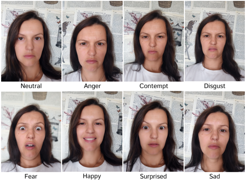
本实验数据集来源于Kaggle,该数据集包含捕捉人们展现七种不同情绪(愤怒、轻蔑、厌恶、恐惧、快乐、悲伤和惊讶)的图像。数据集中的每张图像代表一种特定的情绪,使研究人员和机器学习从业者能够研究和开发用于情绪识别和分析的模型。
3.技术工具
Python版本:3.9
代码编辑器:jupyter notebook
4.实验过程
4.1导入数据
在正式开始模型训练之前,需要先导入项目中用到的各类Python库,并读取实验所使用的数据集。这些库主要包括数据处理(如NumPy、Pandas)、数据可视化(如Matplotlib、Seaborn)、图像处理(如OpenCV、PIL、skimage)、机器学习工具(如Scikit-learn),以及深度学习框架TensorFlow/Keras等。完成库的加载后,再通过pandas读取存储在CSV文件中的面部表情数据集,为后续的数据预处理、模型构建和训练做好准备。
# ==============================
# 导入项目所需的各类Python库
# ==============================

# 数值计算库,用于数组和矩阵运算
import numpy as np

# 数据分析与数据表处理库
import pandas as pd

# 数据可视化库,用于绘制图表
import matplotlib.pyplot as plt

# 基于matplotlib的统计数据可视化库
import seaborn as sns

# 忽略运行过程中产生的一些警告信息
import warnings

# 用于批量读取文件路径
import glob

# 用于读取图像文件
from skimage.io import imread

# OpenCV库,用于图像处理与计算机视觉任务
import cv2

# Python图像处理库
from PIL import Image

# 图像尺寸调整函数
from skimage.transform import resize

# 迭代工具库
import itertools

# Keras中的图像数据增强工具
from tensorflow.keras.preprocessing.image import ImageDataGenerator

# 标签编码工具,用于将类别标签转换为数值形式
from sklearn.preprocessing import LabelEncoder

# 用于将数据集划分为训练集和测试集
from sklearn.model_selection import train_test_split

# Adam优化器,用于模型训练中的参数更新
from tensorflow.keras.optimizers import Adam

# 分类交叉熵指标
from keras.metrics import categorical_crossentropy

# 早停机制,当模型在验证集上不再提升时提前停止训练
from tensorflow.keras.callbacks import EarlyStopping, ReduceLROnPlateau

# 将标签转换为独热编码(one-hot)
from tensorflow.keras.utils import to_categorical

# 导入预训练的ResNet50模型
from tensorflow.keras.applications import ResNet50

# Keras中的网络层与模型构建模块
from tensorflow.keras import layers, models

# 回调函数:早停与动态调整学习率
from tensorflow.keras.callbacks import EarlyStopping, ReduceLROnPlateau

# 计算混淆矩阵,用于评估分类效果
from sklearn.metrics import confusion_matrix

# 输出分类评估报告(精确率、召回率等指标)
from sklearn.metrics import classification_report

# 用于保存训练好的模型
from tensorflow.keras.models import save_model


# ==============================
# 读取数据集
# ==============================

# 从CSV文件中加载面部表情数据集
# 该数据集包含图像信息以及对应的情绪标签
df = pd.read_csv('/kaggle/input/facial-emotion-recognition/emotions.csv')

# 查看数据集内容
df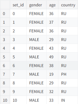
4.2数据可视化

在完成数据读取后,首先对数据集进行简单的可视化分析,以便了解样本的基本分布情况。本部分主要从性别分布、国家分布以及年龄结构三个方面进行统计展示。通过柱状图和饼图可以直观地观察不同类别样本的数量和比例,而直方图与箱线图则用于分析年龄变量在不同性别群体中的分布特征。这些可视化结果有助于初步了解数据结构,并为后续的数据处理和模型训练提供参考。
性别频数分布
# 绘制性别数量分布柱状图

# 设置图像大小
plt.figure(figsize=(10, 8))

# 使用seaborn绘制柱状图
# x轴为性别类别(通过value_counts获取唯一类别)
# y轴为每个性别对应的样本数量
sns.barplot(x=df['gender'].value_counts().index, y=df['gender'].value_counts())

# 设置图表标题
plt.title('Frequency of Gender')

# 设置x轴标签
plt.xlabel('Gender')

# 设置y轴标签
plt.ylabel('Frequency')

# 显示图像
plt.show()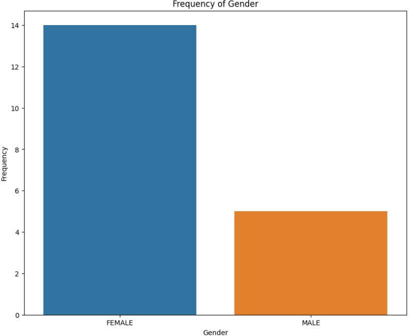
性别比例分布
# 绘制性别比例饼图

# 设置图像大小
plt.figure(figsize=(10, 8))

# 绘制饼图
# value_counts()用于统计每个性别的数量
# labels表示每个扇区的标签
# autopct用于显示百分比
# startangle控制起始角度
# colors设置不同扇区颜色
plt.pie(df['gender'].value_counts(),
        labels=df['gender'].value_counts().index,
        autopct='%1.1f%%',
        startangle=140,
        colors=['skyblue', 'lightcoral'])

# 设置图表标题
plt.title('Proportion of Gender')

# 显示图像
plt.show()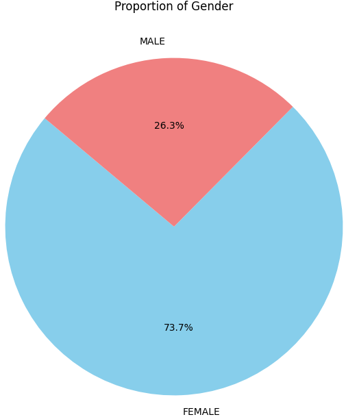
国家比例分布
# 绘制不同国家样本比例的饼图

# 设置图像大小
plt.figure(figsize=(10, 8))

# 绘制饼图
# 统计每个国家对应的样本数量
# labels为国家名称
# autopct显示百分比
# colors设置颜色区分不同国家
plt.pie(df['country'].value_counts(),
        labels=df['country'].value_counts().index,
        autopct='%1.1f%%',
        startangle=140,
        colors=['skyblue', 'lightgreen','lightcoral'])

# 设置图表标题
plt.title('Proportion of Country')

# 显示图像
plt.show()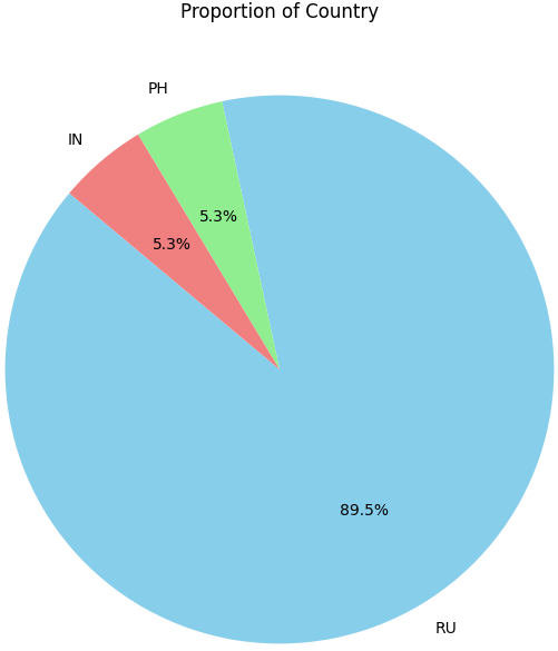
不同性别的年龄分布
# 绘制不同性别的年龄分布直方图

# 忽略未来版本的警告信息,避免输出干扰
warnings.simplefilter(action='ignore', category=FutureWarning)

# 设置图像大小
plt.figure(figsize=(12, 8))

# 使用seaborn绘制直方图
# x表示年龄
# hue表示按照性别进行分类显示
# palette设置颜色风格
# kde=True表示叠加核密度曲线
# bins=20表示划分为20个区间
sns.histplot(data=df, x='age', hue='gender', palette='Set1', kde=True, bins=20)

# 设置标题
plt.title('Histogram of Age by Sex')

# 设置x轴标签
plt.xlabel('Age')

# 设置y轴标签
plt.ylabel('Frequency')

# 显示图像
plt.show()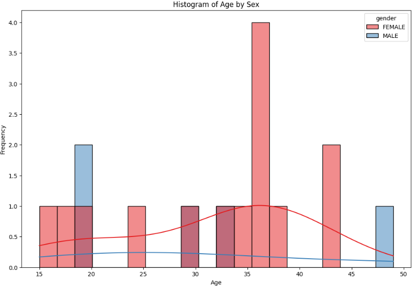
4.3特征工程
在模型训练之前,需要对原始图像数据进行整理和预处理。本部分首先读取数据集中所有图像文件路径,并随机展示部分样本,以直观了解数据内容。随后构建一个新的DataFrame,用于记录每张图像的路径及其对应的情绪标签,并对标签进行统一规范化处理。接着利用 LabelEncoder 将情绪类别转换为数值标签,同时将图像统一调整为224×224大小,以满足ResNet50模型的输入要求。为了提升模型的泛化能力,还使用 ImageDataGenerator 对训练样本进行数据增强,通过旋转、平移、缩放等方式生成新的样本数据。最后将数据划分为训练集和测试集,并将标签转换为独热编码形式,为后续模型训练做好准备。
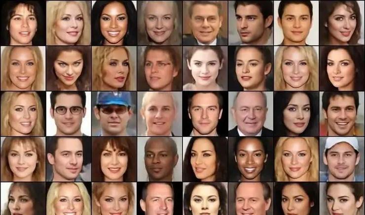
1)读取图像路径并展示部分样本
# ==============================
# 读取数据集中所有图像的路径
# ==============================

# 使用glob批量读取指定目录下所有jpg图像路径
images = glob.glob('/kaggle/input/facial-emotion-recognition/images/*/*.jpg')

# ==============================
# 随机展示部分图像样本
# ==============================

# 创建一个1行5列的子图,用于展示5张示例图片
fig, axes = plt.subplots(1, 5, figsize=(20, 10))

for i in range(5):
    # 使用OpenCV读取图像
    img = cv2.imread(images[i])

    # 在对应子图中显示图像
    axes[i].imshow(img)

# 显示图像
plt.show()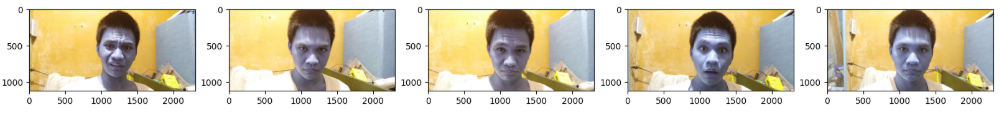
2)构建图像路径与情绪标签数据表
# ==============================
# 构建图像路径与情绪标签的DataFrame
# ==============================

# 创建一个新的DataFrame,用于存储图像路径和情绪标签
image_data = pd.DataFrame(index=np.arange(0, len(images)), columns=['path', 'emotion'])

# 遍历所有图像路径
for i in range(len(images)):

    # 保存图像路径
    image_data.loc[i, 'path'] = images[i]

    # 从路径中提取情绪类别作为标签
    image_data.loc[i, 'emotion'] = images[i][50:].replace(images[i][-4:], '')

# ==============================
# 统一情绪标签格式
# ==============================

# 去除情绪标签中的多余字符,确保标签统一
image_data['emotion'] = image_data['emotion'].replace('/Surprised', 'Surprised')
image_data['emotion'] = image_data['emotion'].replace('/Happy', 'Happy')
image_data['emotion'] = image_data['emotion'].replace('/Sad', 'Sad')
image_data['emotion'] = image_data['emotion'].replace('/Anger', 'Anger')
image_data['emotion'] = image_data['emotion'].replace('/Neutral', 'Neutral')
image_data['emotion'] = image_data['emotion'].replace('/Fear', 'Fear')
image_data['emotion'] = image_data['emotion'].replace('/Contempt', 'Contempt')
image_data['emotion'] = image_data['emotion'].replace('/Disgust', 'Disgust')

# ==============================
# 展示部分样本图像及其标签
# ==============================

# 创建4行10列的子图,总共展示40张图像
fig, axes = plt.subplots(4, 10, figsize=(20, 10))

for i in range(4):
    for j in range(10):

        # 读取图像
        image = imread(image_data.iloc[j + 10*i]["path"])

        # 显示图像
        axes[i, j].imshow(image)

        # 获取对应情绪标签
        label = image_data.iloc[j + 10*i]["emotion"]

        # 在子图上显示标签
        axes[i, j].set_title(label, fontsize=8)

        # 关闭坐标轴
        axes[i, j].axis('off')

# 调整子图间距
plt.tight_layout(rect=[0, 0, 1, 0.96])

# 显示图像
plt.show()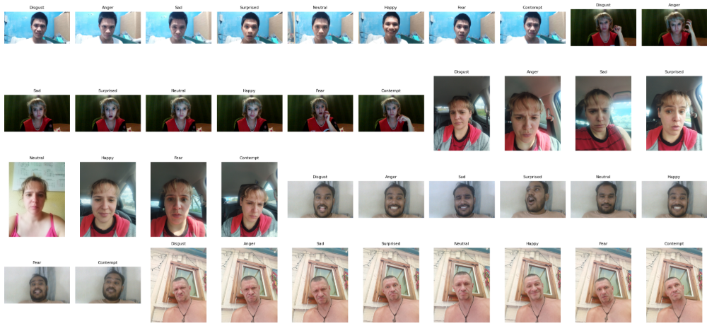
3)标签编码、图像处理与数据增强
# ==============================
# 将情绪标签编码为数值
# ==============================

# 使用LabelEncoder将文本标签转换为整数标签
label_encoder = LabelEncoder()
image_data['emotion'] = label_encoder.fit_transform(image_data['emotion'])


# ==============================
# 读取图像并统一尺寸
# ==============================

# 用于存储图像特征和标签
X = []
y = []

# 遍历DataFrame中的图像路径和标签
for feature, label in image_data.values:

    # 读取图像
    image = cv2.imread(feature)

    # 将图像调整为224×224尺寸(ResNet50模型输入要求)
    image = cv2.resize(image, (224, 224), interpolation = cv2.INTER_LINEAR)

    # 保存图像数据
    X.append(image)

    # 保存标签
    y.append(label)

# 转换为numpy数组
X = np.array(X)
y = np.array(y)


# ==============================
# 数据增强(Data Augmentation)
# ==============================

# 创建ImageDataGenerator对象,用于生成增强样本
datagen = ImageDataGenerator(

    # 随机旋转角度
    rotation_range=30,

    # 水平方向平移
    width_shift_range=0.2,

    # 垂直方向平移
    height_shift_range=0.2,

    # 剪切变换
    shear_range=0.2,

    # 随机缩放
    zoom_range=0.2,

    # 随机水平翻转
    horizontal_flip=True,

    # 填充方式
    fill_mode='nearest'
)


# ==============================
# 生成增强数据
# ==============================

augmented_X = []
augmented_y = []

# 遍历原始数据
for i in range(len(X)):

    # 调整图像维度以适应数据增强函数输入
    img = X[i].reshape((1, *X[i].shape))

    # 获取对应标签
    label = y[i]

    # 每张图像生成50张增强图像
    for _ in range(50):

        # 生成增强图像
        augmented = next(datagen.flow(img, batch_size=1))

        # 保存增强图像
        augmented_X.append(augmented[0])

        # 保存标签
        augmented_y.append(label)


# 转换为numpy数组
augmented_X = np.array(augmented_X)
augmented_y = np.array(augmented_y)


# ==============================
# 合并原始数据与增强数据
# ==============================

X = np.concatenate([X, augmented_X], axis=0)
y = np.concatenate([y, augmented_y], axis=0)


# ==============================
# 划分训练集与测试集
# ==============================

# 按8:2比例划分训练集和测试集
X_train, X_test, y_train, y_test = train_test_split(X, y, test_size = 0.2, random_state=42)


# ==============================
# 标签独热编码
# ==============================

# 将标签转换为one-hot编码形式
y_train = to_categorical(y_train, num_classes = 8)
y_test = to_categorical(y_test, num_classes = 8)
4.4构建模型
在完成数据预处理之后,接下来需要构建用于面部表情识别的深度学习模型。本实验采用迁移学习的方法,以ResNet50作为基础网络结构。ResNet50是一个在ImageNet数据集上预训练的深层卷积神经网络,能够有效提取图像的高层次特征。这里将其作为特征提取器,并冻结其参数,从而减少训练成本并提高训练稳定性。在其后加入全局平均池化层和多个全连接层,用于完成最终的情绪分类任务。同时设置EarlyStopping和ReduceLROnPlateau两个回调函数,用于在训练过程中自动控制训练节奏并防止过拟合。最后对模型进行编译,指定优化器、损失函数和评价指标。
# ==============================
# 构建模型
# ==============================

# EarlyStopping回调函数
# 当验证集准确率在若干轮训练中不再提升时,提前停止训练
early_stopping = EarlyStopping(
    monitor='val_accuracy',        # 监控验证集准确率
    patience=10,                   # 若连续10轮没有提升则停止训练
    mode='max',                    # 以最大值为优化目标
    verbose=1,                     # 输出训练日志
    restore_best_weights=True      # 恢复表现最好的模型权重
)

# ReduceLROnPlateau回调函数
# 当验证集准确率不再提升时自动降低学习率
lr_reduction = ReduceLROnPlateau(
    monitor='val_accuracy',        # 监控验证集准确率
    patience=3,                    # 若连续3轮无提升则降低学习率
    mode='max',                    # 以最大值为优化目标
    verbose=1,                     # 输出调整信息
    factor=0.5,                    # 学习率降低为原来的0.5倍
    min_lr=0.0001                  # 设置学习率下限
)

# ==============================
# 加载ResNet50预训练模型
# ==============================

# 加载在ImageNet数据集上训练好的ResNet50模型
# include_top=False 表示去掉原有的全连接分类层
# input_shape指定输入图像大小为224×224×3
base_model = ResNet50(
    weights='imagenet',
    include_top=False,
    input_shape=(224, 224, 3)
)

# 冻结ResNet50网络参数,使其仅作为特征提取器
base_model.trainable = False


# ==============================
# 构建完整分类模型
# ==============================

# 使用Sequential方式堆叠网络结构
model = models.Sequential([

    # 预训练的ResNet50特征提取网络
    base_model,

    # 全局平均池化层,用于将卷积特征图转换为一维特征向量
    layers.GlobalAveragePooling2D(),

    # 全连接层,用于学习更高层的特征表示
    layers.Dense(512, activation='relu'),

    # 第二个全连接层
    layers.Dense(256, activation='relu'),

    # Dropout层,用于减少过拟合
    layers.Dropout(0.3),

    # 输出层,共8个情绪类别,使用softmax进行多分类
    layers.Dense(8, activation='softmax')
])


# ==============================
# 编译模型
# ==============================

# 指定优化器、损失函数以及评价指标
model.compile(
    optimizer='adam',                     # 使用Adam优化器
    loss='categorical_crossentropy',      # 多分类交叉熵损失函数
    metrics=['accuracy']                  # 评估指标为准确率
)

# 输出模型结构信息
model.summary()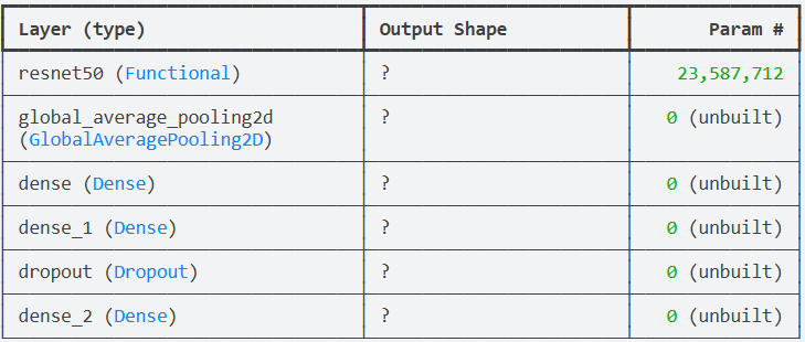
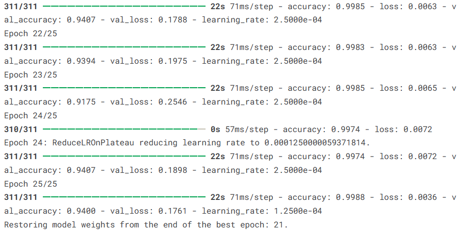
4.5训练模型
在模型结构构建完成并编译之后,接下来需要使用训练数据对模型进行训练。训练过程中,模型会不断调整网络参数,使预测结果逐渐逼近真实标签。本实验使用训练集 X_train 和 y_train 进行模型训练,同时使用测试集作为验证集,在每一轮训练结束后评估模型在验证集上的表现。训练过程中设置批量大小(batch size)为20,并进行25轮迭代训练。此外,在训练时引入了早停(EarlyStopping)和学习率动态调整(ReduceLROnPlateau)两个回调函数,用于在模型性能不再提升时自动停止训练或降低学习率,从而提高训练效率并减少过拟合风险。
# ==============================
# 训练模型
# ==============================

# 使用训练数据对模型进行训练
history = model.fit(

    # 训练集特征数据
    X_train,

    # 训练集标签数据
    y_train,

    # 每次训练使用的样本数量(批大小)
    batch_size=20,

    # 验证集数据,用于在训练过程中评估模型性能
    validation_data=(X_test, y_test),

    # 训练轮数(epochs),表示完整遍历训练数据的次数
    epochs=25,

    # 回调函数列表
    # early_stopping:当验证集准确率不再提升时提前停止训练
    # lr_reduction:当模型性能停滞时自动降低学习率
    callbacks=[early_stopping, lr_reduction]
)
4.6模型评估
在模型训练完成后,需要对模型的性能进行系统评估。本部分首先使用测试集对模型进行整体评估,得到模型在未参与训练数据上的准确率和损失值。随后通过分类报告(classification report)计算各类别的精确率(Precision)、召回率(Recall)和F1-score,以更全面地衡量模型在不同情绪类别上的识别效果。接着绘制混淆矩阵,通过可视化方式观察模型在各类别之间的预测情况。最后绘制模型训练过程中的准确率曲线和损失曲线,以分析模型在训练集和验证集上的学习趋势,从而判断模型是否存在过拟合或欠拟合情况。
1)模型整体评估
# ==============================
# 在测试集上评估模型性能
# ==============================

# 使用测试数据评估模型,返回损失值和准确率
loss, accuracy = model.evaluate(X_test, y_test)

# 输出模型在测试集上的准确率
print("Test Accuracy:", accuracy)

# 输出模型在测试集上的损失值
print("Loss:", loss)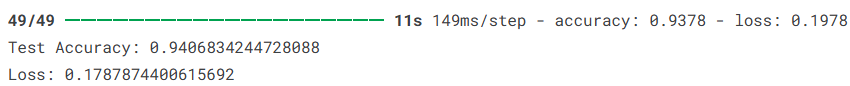
2)分类报告(Classification Report)
# ==============================
# 生成分类报告
# ==============================

# 使用训练好的模型对测试集进行预测
y_pred = model.predict(X_test)

# 将one-hot编码形式的真实标签转换为类别索引
y_test = np.argmax(y_test, axis=1)

# 将预测概率转换为预测类别
y_pred_classes = np.argmax(y_pred, axis=1)

# 输出分类报告
# 包括每个类别的Precision、Recall、F1-score等指标
print(classification_report(y_test, y_pred_classes))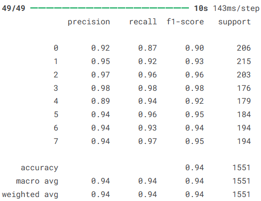
3)混淆矩阵(Confusion Matrix)
# ==============================
# 绘制混淆矩阵
# ==============================

# 计算混淆矩阵
confusion_mtx = confusion_matrix(y_test, y_pred_classes)

# 创建画布
f,ax = plt.subplots(figsize=(8, 8))

# 使用seaborn绘制热力图
sns.heatmap(confusion_mtx,
            annot=True,              # 显示具体数值
            linewidths=0.01,         # 网格线宽度
            cmap="BuPu",             # 颜色风格
            linecolor="gray",        # 网格颜色
            fmt= '.1f',              # 数值格式
            ax=ax)

# 设置x轴标签
plt.xlabel("Predicted Label")

# 设置y轴标签
plt.ylabel("True Label")

# 设置标题
plt.title("Confusion Matrix")

# 显示图像
plt.show()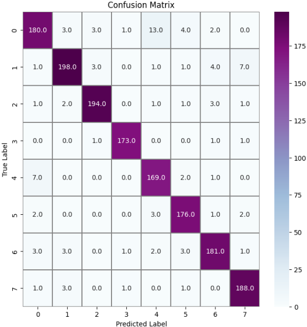
4)准确率变化曲线
# ==============================
# 绘制训练过程中的准确率变化
# ==============================

# 设置图像大小
plt.figure(figsize=(20, 8))

# 绘制训练集准确率
plt.plot(history.history['accuracy'])

# 绘制验证集准确率
plt.plot(history.history['val_accuracy'])

# 设置图表标题
plt.title('Model Accuracy')

# 设置y轴标签
plt.ylabel('accuracy')

# 设置x轴标签
plt.xlabel('epoch')

# 设置图例
plt.legend(['train', 'test'], loc='upper left')

# 显示图像
plt.show()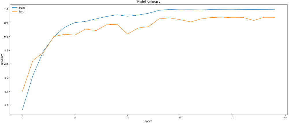
5)损失变化曲线
# ==============================
# 绘制训练过程中的损失变化
# ==============================

# 设置图像大小
plt.figure(figsize=(20, 8))

# 绘制训练集损失值
plt.plot(history.history['loss'])

# 绘制验证集损失值
plt.plot(history.history['val_loss'])

# 设置图表标题
plt.title('Model Loss')

# 设置y轴标签
plt.ylabel('loss')

# 设置x轴标签
plt.xlabel('epoch')

# 设置图例
plt.legend(['train', 'test'], loc='upper left')

# 显示图像
plt.show()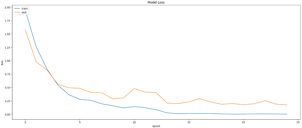
最后可以保存模型
model.save('facial_emotion_recognition_model.h5')5.总结
本文基于Kaggle公开的人脸情绪识别数据集,构建并实现了一个基于ResNet50的面部表情分类模型。该数据集包含愤怒、轻蔑、厌恶、恐惧、快乐、悲伤和惊讶等多种情绪类别,为情绪识别任务提供了较为丰富的训练样本。在实验过程中,首先对图像数据进行了整理与增强处理,然后利用迁移学习方法引入预训练的ResNet50网络进行特征提取,并在其基础上构建全连接分类层完成情绪识别任务。实验结果表明,模型在测试集上取得了94.07%的准确率,损失值为0.1788,各类别的Precision、Recall和F1-score整体均保持在较高水平,宏平均和加权平均均达到0.94,说明模型在不同情绪类别上的识别能力较为稳定。总体来看,该方法能够较好地提取面部图像中的情绪特征,在面部表情识别任务中表现出较好的分类效果,为后续进一步优化模型结构和提升识别性能提供了参考。
源代码
# Importing libraries for data handling, visualization, and deep learning
import numpy as np
import pandas as pd
import matplotlib.pyplot as plt
import seaborn as sns
import warnings
import glob
from skimage.io import imread
import cv2
from PIL import Image
from skimage.transform import resize
import itertools
from tensorflow.keras.preprocessing.image import ImageDataGenerator
from sklearn.preprocessing import LabelEncoder
from sklearn.model_selection import train_test_split
from tensorflow.keras.optimizers import Adam
from keras.metrics import categorical_crossentropy
from tensorflow.keras.callbacks import EarlyStopping, ReduceLROnPlateau
from tensorflow.keras.utils import to_categorical
from tensorflow.keras.applications import ResNet50
from tensorflow.keras import layers, models
from tensorflow.keras.callbacks import EarlyStopping, ReduceLROnPlateau
from sklearn.metrics import confusion_matrix
from sklearn.metrics import classification_report
from tensorflow.keras.models import save_model
# Loading the dataset
df = pd.read_csv('/kaggle/input/facial-emotion-recognition/emotions.csv')
df
# Plotting the frequency of gender
plt.figure(figsize=(10, 8))
sns.barplot(x=df['gender'].value_counts().index, y=df['gender'].value_counts())
plt.title('Frequency of Gender')
plt.xlabel('Gender')
plt.ylabel('Frequency')
plt.show()
# Plotting the proportion of gender using a pie chart
plt.figure(figsize=(10, 8))
plt.pie(df['gender'].value_counts(), labels=df['gender'].value_counts().index, autopct='%1.1f%%', startangle=140,
        colors=['skyblue', 'lightcoral'])
plt.title('Proportion of Gender')
plt.show()
# Plotting the proportion of country using a pie chart
plt.figure(figsize=(10, 8))
plt.pie(df['country'].value_counts(), labels=df['country'].value_counts().index, autopct='%1.1f%%', startangle=140,
        colors=['skyblue', 'lightgreen','lightcoral'])
plt.title('Proportion of Country')
plt.show()
# Visualizing the age distribution by gender
warnings.simplefilter(action='ignore', category=FutureWarning)
plt.figure(figsize=(12, 8))
sns.histplot(data=df, x='age', hue='gender', palette='Set1', kde=True, bins=20)
plt.title('Histogram of Age by Sex')
plt.xlabel('Age')
plt.ylabel('Frequency')
plt.show()
# Boxplot for age distribution by gender
plt.figure(figsize=(10, 8))
df.boxplot(column='age', by='gender', patch_artist=True, boxprops=dict(facecolor='skyblue', color='blue'),
           medianprops=dict(color='red'))
plt.title('Boxplot of Age by Gender')
plt.suptitle('')
plt.xlabel('Gender')
plt.ylabel('Age')
plt.show()
# Loading image paths
images = glob.glob('/kaggle/input/facial-emotion-recognition/images/*/*.jpg')
# Displaying some sample images
fig, axes = plt.subplots(1, 5, figsize=(20, 10))
for i in range(5):
    img = cv2.imread(images[i])
    axes[i].imshow(img)
plt.show()
# Creating a DataFrame for image paths and their respective emotions
image_data = pd.DataFrame(index=np.arange(0, len(images)), columns=['path', 'emotion'])
for i in range(len(images)):
    image_data.loc[i, 'path'] = images[i]
    image_data.loc[i, 'emotion'] = images[i][50:].replace(images[i][-4:], '')
# Standardizing the emotion column values by removing unnecessary prefixes to ensure consistency in emotion labels.
image_data['emotion'] = image_data['emotion'].replace('/Surprised', 'Surprised')
image_data['emotion'] = image_data['emotion'].replace('/Happy', 'Happy')
image_data['emotion'] = image_data['emotion'].replace('/Sad', 'Sad')
image_data['emotion'] = image_data['emotion'].replace('/Anger', 'Anger')
image_data['emotion'] = image_data['emotion'].replace('/Neutral', 'Neutral')
image_data['emotion'] = image_data['emotion'].replace('/Fear', 'Fear')
image_data['emotion'] = image_data['emotion'].replace('/Contempt', 'Contempt')
image_data['emotion'] = image_data['emotion'].replace('/Disgust', 'Disgust')
# Displaying a grid of 40 images (4 rows and 10 columns) with their corresponding emotion labels
fig, axes = plt.subplots(4, 10, figsize=(20, 10))
for i in range(4):
    for j in range(10):
        image = imread(image_data.iloc[j + 10*i]["path"])
        axes[i, j].imshow(image)
        label = image_data.iloc[j + 10*i]["emotion"]
        axes[i, j].set_title(label, fontsize=8)
        axes[i, j].axis('off')
plt.tight_layout(rect=[0, 0, 1, 0.96])
plt.show()
# Encoding the emotion labels as integers using LabelEncoder
label_encoder = LabelEncoder()
image_data['emotion'] = label_encoder.fit_transform(image_data['emotion'])
# Loading and resizing images to 224x224 pixels and preparing feature (X) and label (y) arrays
X = []
y = []
for feature, label in image_data.values:
    image = cv2.imread(feature)
    image = cv2.resize(image, (224, 224), interpolation = cv2.INTER_LINEAR)
    X.append(image)
    y.append(label)
X = np.array(X)
y = np.array(y)
# Data augmentation using ImageDataGenerator
datagen = ImageDataGenerator(
    rotation_range=30,
    width_shift_range=0.2,
    height_shift_range=0.2,
    shear_range=0.2,
    zoom_range=0.2,
    horizontal_flip=True,
    fill_mode='nearest'
)
# Applying augmentation to images
augmented_X = []
augmented_y = []
for i in range(len(X)):
    img = X[i].reshape((1, *X[i].shape))
    label = y[i]
    for _ in range(50):
        augmented = next(datagen.flow(img, batch_size=1))
        augmented_X.append(augmented[0])
        augmented_y.append(label)
augmented_X = np.array(augmented_X)
augmented_y = np.array(augmented_y)
# Combining original and augmented data
X = np.concatenate([X, augmented_X], axis=0)
y = np.concatenate([y, augmented_y], axis=0)
# Splitting data into training and testing sets
X_train, X_test, y_train, y_test = train_test_split(X, y, test_size = 0.2, random_state=42)
y_train = to_categorical(y_train, num_classes = 8)
y_test = to_categorical(y_test, num_classes = 8)
# Building the model
early_stopping = EarlyStopping(monitor='val_accuracy', patience=10, mode='max', verbose=1, restore_best_weights=True)
lr_reduction = ReduceLROnPlateau(monitor='val_accuracy', patience=3, mode='max', verbose=1, factor=0.5, min_lr=0.0001)
base_model = ResNet50(weights='imagenet', include_top=False, input_shape=(224, 224, 3))
base_model.trainable = False
model = models.Sequential([
    base_model,
    layers.GlobalAveragePooling2D(),
    layers.Dense(512, activation='relu'),
    layers.Dense(256, activation='relu'),
    layers.Dropout(0.3),
    layers.Dense(8, activation='softmax')
])
# Compiling the model
model.compile(optimizer='adam', loss='categorical_crossentropy', metrics=['accuracy'])
model.summary()
# Training the model
history = model.fit(
    X_train, y_train, batch_size=20, validation_data=(X_test, y_test), epochs=25, callbacks=[early_stopping, lr_reduction]
)
# Evaluating the model
loss, accuracy = model.evaluate(X_test, y_test)
print("Test Accuracy:", accuracy)
print("Loss:", loss)
# Classification report
y_pred = model.predict(X_test)
y_test = np.argmax(y_test, axis=1)
y_pred_classes = np.argmax(y_pred, axis=1)
print(classification_report(y_test, y_pred_classes))
# Confusion matrix
confusion_mtx = confusion_matrix(y_test, y_pred_classes)
f,ax = plt.subplots(figsize=(8, 8))
sns.heatmap(confusion_mtx, annot=True, linewidths=0.01,cmap="BuPu",linecolor="gray", fmt= '.1f',ax=ax)
plt.xlabel("Predicted Label")
plt.ylabel("True Label")
plt.title("Confusion Matrix")
plt.show()
# Accuracy plot
plt.figure(figsize=(20, 8))
plt.plot(history.history['accuracy'])
plt.plot(history.history['val_accuracy'])
plt.title('Model Accuracy')
plt.ylabel('accuracy')
plt.xlabel('epoch')
plt.legend(['train', 'test'], loc='upper left')
plt.show()
# Loss plot
plt.figure(figsize=(20, 8))
plt.plot(history.history['loss'])
plt.plot(history.history['val_loss'])
plt.title('Model Loss')
plt.ylabel('loss')
plt.xlabel('epoch')
plt.legend(['train', 'test'], loc='upper left')
plt.show()
model.save('facial_emotion_recognition_model.h5')
资料获取,更多粉丝福利,关注下方公众号获取


AtomGit 是由开放原子开源基金会联合 CSDN 等生态伙伴共同推出的新一代开源与人工智能协作平台。平台坚持“开放、中立、公益”的理念,把代码托管、模型共享、数据集托管、智能体开发体验和算力服务整合在一起,为开发者提供从开发、训练到部署的一站式体验。
更多推荐


 1
1 0
0- 0


 已为社区贡献5条内容

所有评论(0)