深度学习实战-基于VIT+GNN的乳腺超声图像分类识别模型

🤵♂️ 个人主页:@艾派森的个人主页
✍🏻作者简介:Python学习者
🐋 希望大家多多支持,我们一起进步!😄
如果文章对你有帮助的话,
欢迎评论 💬点赞👍🏻 收藏 📂加关注+
目录
1.项目背景
近年来,随着医学影像技术的快速发展,超声、CT、MRI等影像手段已经成为临床疾病诊断的重要依据。其中,乳腺超声由于具有无创、无辐射、成本较低等优势,被广泛应用于乳腺疾病的早期筛查与辅助诊断。然而,乳腺超声图像通常具有噪声多、对比度低、边界模糊等特点,对医生的阅片经验和专业能力依赖较高,在实际诊断过程中容易受到主观因素影响。因此,如何利用计算机技术对乳腺超声图像进行自动分析与识别,成为近年来医学影像智能化研究的重要方向。
随着深度学习技术的发展,基于卷积神经网络(CNN)的医学图像分类方法在乳腺肿瘤检测、病灶识别等任务中取得了较好的效果。但传统CNN模型主要依赖局部卷积操作提取特征,在处理复杂结构关系或全局信息时仍存在一定局限。近年来,Transformer结构在计算机视觉领域逐渐兴起,其中Vision Transformer(ViT)通过自注意力机制能够更好地建模图像的全局特征关系,在多种视觉任务中表现出较强的特征表达能力。同时,图神经网络(Graph Neural Network,GNN)在处理结构化数据和关系信息方面具有独特优势,可以通过构建节点之间的连接关系来捕捉更丰富的结构特征。
在此背景下,将Vision Transformer与图神经网络相结合,为医学影像分析提供了一种新的建模思路。通过先利用ViT对图像进行特征提取,再借助GNN刻画图像patch之间的潜在结构关系,有望进一步提升模型对复杂医学影像特征的表达能力。基于这一思路,本文以公开的乳腺超声图像数据集为研究对象,构建了一个融合ViT与GNN的乳腺超声图像分类模型,对正常、良性和恶性三类乳腺组织进行自动识别,并通过实验评估模型在乳腺疾病辅助诊断中的应用效果。
2.数据集介绍
本实验数据集来源于Kaggle,该数据集收集了25至75岁女性的基线乳腺超声图像。数据整理于2018年,共纳入600名女性患者。数据集包含780张图像,平均图像大小为500×500像素,格式为PNG。图像中包含原始图像作为对照。图像被分为三类:正常、良性和恶性。
3.技术工具
Python版本:3.9
代码编辑器:jupyter notebook
4.实验过程
4.1导入数据
在构建乳腺超声图像分类模型之前,需要首先完成数据集的读取与整理。本步骤的主要任务是从数据目录中遍历不同类别的图像文件,提取图像路径及其对应的掩膜(mask)文件,并建立统一的数据结构用于后续处理。由于该数据集同时包含原始超声图像和对应的标注掩膜,因此在读取过程中需要确保图像与掩膜文件能够正确配对,从而保证数据完整性。最终,通过构建数据表的方式将图像路径、掩膜路径以及肿瘤类型标签进行统一管理,为后续的数据预处理和模型训练提供结构化的数据基础。
import numpy as np
import pandas as pd
import os

# 数据集根目录
base_path = '/kaggle/input/breast-ultrasound-images-dataset/Dataset_BUSI_with_GT/'

# 三种乳腺超声图像类别:良性、恶性、正常
tumor_types = ["benign", "malignant", "normal"]

# 用于存储图像路径、掩膜路径和类别标签
image_paths = []
mask_paths = []
tumor_labels = []

# 遍历每一种肿瘤类型的文件夹
for tumor in tumor_types:

    # 构建当前类别文件夹路径
    folder_path = os.path.join(base_path, tumor)

    # 判断文件夹是否存在
    if os.path.exists(folder_path):

        # 获取当前文件夹下所有文件
        files = os.listdir(folder_path)

        # 只保留原始图像文件(排除mask文件)
        image_files = [f for f in files if f.endswith(".png") and "_mask" not in f]

        # 遍历每一张图像
        for img_file in image_files:

            # 根据图像文件名生成对应的mask文件名
            mask_file = img_file.replace(".png", "_mask.png")

            # 构建图像路径和mask路径
            img_path = os.path.join(folder_path, img_file)
            mask_path = os.path.join(folder_path, mask_file)

            # 判断图像和mask是否同时存在
            if os.path.exists(img_path) and os.path.exists(mask_path):

                # 保存图像路径
                image_paths.append(img_path)

                # 保存mask路径
                mask_paths.append(mask_path)

                # 保存类别标签
                tumor_labels.append(tumor)
            else:
                # 若图像或mask缺失则输出提示
                print(f"Missing pair for image: {img_path} or mask: {mask_path}")

    else:
        # 若类别文件夹不存在则输出提示
        print(f"Folder not found: {folder_path}")

# 将整理好的数据构建为DataFrame结构
df = pd.DataFrame({
    "image_path": image_paths,
    "mask_path": mask_paths,
    "tumor_type": tumor_labels
})

# 查看数据表
df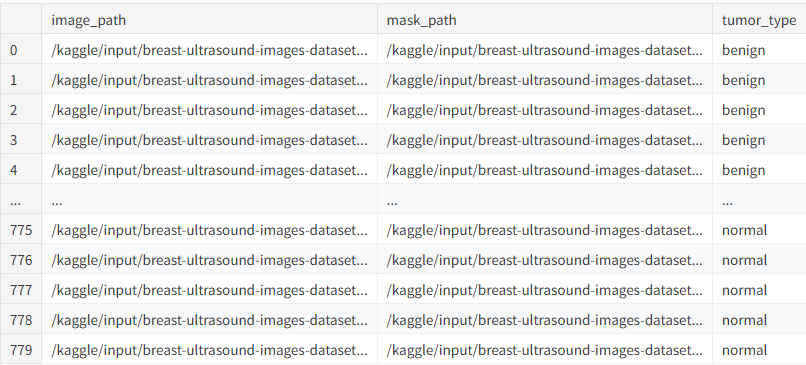
4.2数据可视化

在完成数据整理后,需要对数据集的基本结构进行初步观察,以了解不同类别样本的数量分布情况。通过可视化方式可以直观地判断数据是否存在明显的类别不平衡问题,这对于后续模型训练具有重要参考价值。本节首先通过柱状图展示各类乳腺超声图像的样本数量,并在图中标注具体数值,以便清晰比较不同类别之间的规模差异。
import seaborn as sns
import matplotlib.pyplot as plt

# 设置Seaborn绘图风格
sns.set_style("whitegrid")

# 创建绘图画布
fig, ax = plt.subplots(figsize=(8, 6))

# 绘制不同肿瘤类型的样本数量柱状图
sns.countplot(data=df, x="tumor_type", palette="viridis", ax=ax)

# 设置图标题和坐标轴标签
ax.set_title("Distribution of Disease Types", fontsize=14, fontweight='bold')
ax.set_xlabel("Tumor Type", fontsize=12)
ax.set_ylabel("Count", fontsize=12)

# 在柱状图上方标注具体数量
for p in ax.patches:
    ax.annotate(
        f'{int(p.get_height())}',  # 标注样本数量
        (p.get_x() + p.get_width() / 2., p.get_height()),
        ha='center',
        va='bottom',
        fontsize=11,
        color='black',
        xytext=(0, 5),
        textcoords='offset points'
    )

# 显示图像
plt.show()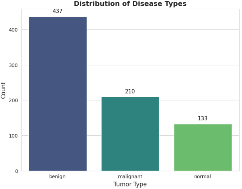
为了进一步从比例角度观察数据分布情况,下面使用饼图展示不同肿瘤类型在整体数据集中的占比。相比柱状图,饼图更适合展示各类别在总体中的相对比例,可以更加直观地反映数据结构特征。
# 统计各类别样本数量
label_counts = df["tumor_type"].value_counts()

# 创建画布
fig, ax = plt.subplots(figsize=(20, 8))

# 设置颜色方案
colors = sns.color_palette("viridis", len(label_counts))

# 绘制饼图
ax.pie(
    label_counts,
    labels=label_counts.index,
    autopct='%1.1f%%',        # 显示百分比
    startangle=140,           # 设置起始角度
    colors=colors,
    textprops={'fontsize': 12, 'weight': 'bold'},
    wedgeprops={'edgecolor': 'black', 'linewidth': 1}
)

# 设置标题
ax.set_title("Distribution of Disease Types - Pie Chart", fontsize=14, fontweight='bold')

# 显示图像
plt.show()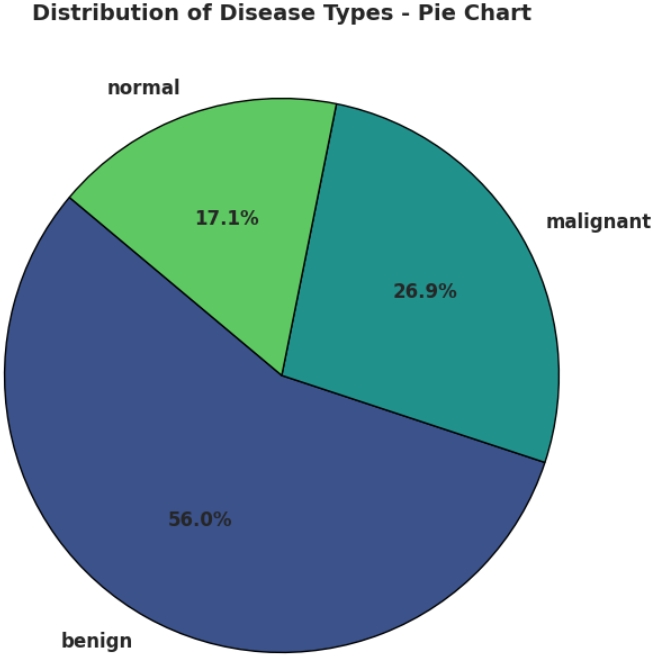
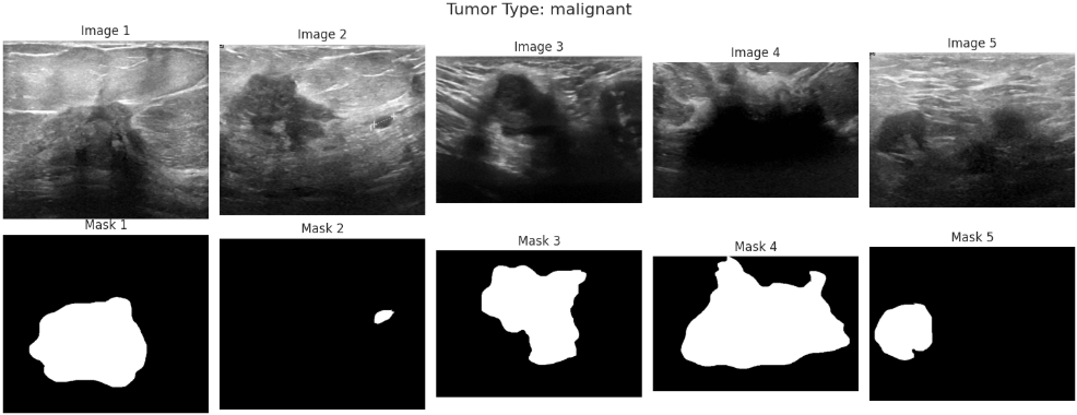
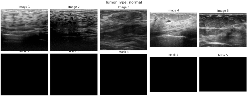
在了解数据集的类别分布之后,还需要进一步观察具体图像样本及其对应的标注信息。乳腺超声数据集中不仅包含原始图像,还提供了对应的病灶掩膜(mask),这些掩膜标注能够指示病灶区域的位置,对于后续模型学习病变区域特征具有重要意义。因此,通过随机抽取不同类别样本并同时展示原始图像与对应掩膜,可以直观了解数据质量以及标注的准确性,从而为后续模型设计和训练提供更加清晰的参考。
import matplotlib.pyplot as plt
import cv2

# 每个类别随机展示的样本数量
n_samples = 5

# 获取数据集中所有肿瘤类型
tumor_types = df['tumor_type'].unique()

# 遍历每一种肿瘤类型
for tumor in tumor_types:

    # 从当前类别中随机抽取若干样本
    subset = df[df['tumor_type'] == tumor].sample(
        n=min(n_samples, len(df[df['tumor_type'] == tumor])),
        random_state=42
    )

    # 创建绘图画布,两行分别显示原始图像和对应的mask
    fig, axs = plt.subplots(2, n_samples, figsize=(3 * n_samples, 6))

    # 设置整体标题
    fig.suptitle(f"Tumor Type: {tumor}", fontsize=16)

    # 遍历样本进行可视化
    for i, (idx, row) in enumerate(subset.iterrows()):

        # 读取原始超声图像(灰度模式)
        image = cv2.imread(row['image_path'], cv2.IMREAD_GRAYSCALE)

        # 读取对应的病灶掩膜图像
        mask = cv2.imread(row['mask_path'], cv2.IMREAD_GRAYSCALE)

        # 显示原始图像
        axs[0, i].imshow(image, cmap='gray')
        axs[0, i].axis('off')
        axs[0, i].set_title(f"Image {i+1}")

        # 显示对应的掩膜图像
        axs[1, i].imshow(mask, cmap='gray')
        axs[1, i].axis('off')
        axs[1, i].set_title(f"Mask {i+1}")

    # 调整子图布局
    plt.tight_layout()

    # 显示图像
    plt.show()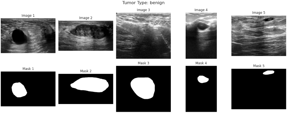
4.3特征工程
在完成数据的初步探索与可视化之后,需要对数据集进行进一步处理,以提高模型训练的稳定性和泛化能力。乳腺超声图像数据集中不同类别样本数量往往存在不均衡问题,如果直接用于模型训练,模型可能会倾向于学习样本数量较多的类别特征,从而影响整体分类性能。因此,在特征工程阶段需要对数据进行类别均衡处理,通过过采样方式扩充样本数量较少的类别,使各类别样本规模保持一致。同时,由于后续模型主要用于图像分类任务,因此只保留图像路径和类别标签信息即可,掩膜路径在当前任务中不再参与训练。经过上述处理,可以构建一个类别更加均衡、结构更加清晰的数据集,为后续模型训练奠定基础。
# 从原始数据集中分别提取三类样本
df_benign = df[df["tumor_type"] == "benign"]       # 良性肿瘤
df_malignant = df[df["tumor_type"] == "malignant"] # 恶性肿瘤
df_normal = df[df["tumor_type"] == "normal"]       # 正常样本

# 计算三个类别中的最大样本数量
# 后续将以该数量作为各类别统一的样本规模
max_size = max(len(df_benign), len(df_malignant), len(df_normal))

from sklearn.utils import resample

# 对恶性肿瘤类别进行过采样
# replace=True 表示允许有放回采样,从而扩充样本数量
df_malignant_oversampled = resample(
    df_malignant,
    replace=True,
    n_samples=max_size,
    random_state=42
)

# 对正常类别进行过采样
df_normal_oversampled = resample(
    df_normal,
    replace=True,
    n_samples=max_size,
    random_state=42
)

# 将三个类别的数据合并为新的平衡数据集
df_balanced = pd.concat([
    df_benign,
    df_malignant_oversampled,
    df_normal_oversampled
])

# 打乱数据顺序,避免同一类别集中出现
df_balanced = df_balanced.sample(frac=1, random_state=42).reset_index(drop=True)

# 用平衡后的数据替换原始数据集
df = df_balanced

# 删除mask路径,因为当前任务只需要图像路径和类别标签
df = df.drop(['mask_path'], axis=1)
通过上述处理后,原本存在类别不均衡问题的数据集被重新构建为一个更加均衡的数据结构,各类别样本数量保持一致。这种处理方式能够减少模型训练过程中对多数类的偏置,使模型在学习不同类别特征时更加充分。同时,通过随机打乱数据顺序可以避免训练过程中出现类别连续分布的问题,而删除不必要的掩膜路径信息则使数据结构更加简洁,为后续的数据加载与模型训练提供了更高效的数据基础。
4.4构建模型
本研究采用 Vision Transformer(ViT)与图神经网络(GNN)相结合的深度学习模型对乳腺超声图像进行分类。首先利用预训练的ViT模型对输入图像进行特征提取,将图像划分为多个固定大小的patch,并通过Transformer结构获取每个patch的高维语义表示。由于医学图像中不同区域之间往往存在空间关联关系,因此在获得patch特征后,将每个patch视为图中的节点,构建图结构,并利用图卷积网络(Graph Convolutional Network,GCN)对patch之间的关系进行建模。
在模型结构中,ViT部分主要负责图像特征提取,而GNN部分用于学习patch之间的结构关系。具体而言,首先通过ViT模型得到每个patch的特征向量,然后构建完全图结构,使每个patch节点之间均建立连接。随后通过两层GCN网络进行特征传播和更新,并通过ReLU函数进行非线性激活。最后对所有节点特征进行全局平均池化,得到图级表示,并通过全连接层输出最终分类结果。
在模型训练过程中,首先将数据集按8:2比例划分为训练集和测试集,并采用交叉熵损失函数(CrossEntropyLoss)作为优化目标,利用AdamW优化器进行参数更新。训练过程中记录每个epoch的损失值和分类准确率,以评估模型的学习效果。训练完成后,在测试集上对模型进行评估,通过计算预测结果与真实标签之间的一致性得到模型的测试准确率,从而评价模型在乳腺肿瘤分类任务中的性能。
# =========================
# 导入相关库
# =========================
import torch
import torch.nn as nn
import torch.optim as optim
from torch.utils.data import Dataset, DataLoader

from torchvision import transforms
from PIL import Image
import pandas as pd

from sklearn.model_selection import train_test_split
from sklearn.preprocessing import LabelEncoder
from sklearn.metrics import confusion_matrix, classification_report

import seaborn as sns
import matplotlib.pyplot as plt
import numpy as np

# ViT模型(Vision Transformer)
from transformers import ViTModel, ViTFeatureExtractor

# 图神经网络
from torch_geometric.nn import GCNConv


# =========================
# 参数设置
# =========================
IMAGE_SIZE = 224        # 输入图像尺寸
BATCH_SIZE = 16         # 每批次样本数量
NUM_EPOCHS = 10         # 训练轮数
LEARNING_RATE = 1e-4    # 学习率
NUM_CLASSES = 3         # 分类类别数量

# 使用预训练ViT模型
VIT_MODEL_NAME = "google/vit-base-patch16-224-in21k"

PATCH_SIZE = 16         # ViT图像patch大小
NUM_PATCHES = (IMAGE_SIZE // PATCH_SIZE) * (IMAGE_SIZE // PATCH_SIZE)

GNN_HIDDEN_DIM = 128    # GNN隐藏层维度


# =========================
# 自定义数据集
# =========================
class BreastUltrasoundDataset(Dataset):

    def __init__(self, dataframe, transform=None):

        self.dataframe = dataframe
        self.transform = transform

        # 将字符串标签编码为数字
        self.label_encoder = LabelEncoder()

        self.dataframe['tumor_type_encoded'] = \
            self.label_encoder.fit_transform(self.dataframe['tumor_type'])

        self.classes = self.label_encoder.classes_

    def __len__(self):
        # 返回数据集大小
        return len(self.dataframe)

    def __getitem__(self, idx):

        # 获取图像路径
        img_path = self.dataframe.iloc[idx]['image_path']

        # 读取图像
        image = Image.open(img_path).convert('RGB')

        # 获取标签
        label = self.dataframe.iloc[idx]['tumor_type_encoded']

        # 图像预处理
        if self.transform:
            image = self.transform(image)

        return image, label


# =========================
# 图像预处理
# =========================
transform = transforms.Compose([

    transforms.Resize((IMAGE_SIZE, IMAGE_SIZE)),  # 调整图像尺寸

    transforms.ToTensor(),                        # 转换为Tensor

    # 使用ImageNet均值和方差进行标准化
    transforms.Normalize(
        mean=[0.485, 0.456, 0.406],
        std=[0.229, 0.224, 0.225]
    ),

])


# =========================
# 构建ViT + GNN分类模型
# =========================
class ViTGNNClassifier(nn.Module):

    def __init__(self,
                 num_classes,
                 vit_model_name=VIT_MODEL_NAME,
                 gnn_hidden_dim=GNN_HIDDEN_DIM,
                 patch_size=PATCH_SIZE):

        super(ViTGNNClassifier, self).__init__()

        # 加载预训练ViT模型
        self.vit = ViTModel.from_pretrained(vit_model_name)

        # ViT特征提取器
        self.feature_extractor = ViTFeatureExtractor.from_pretrained(vit_model_name)

        # 冻结ViT参数(只使用其特征提取能力)
        for param in self.vit.parameters():
            param.requires_grad = False

        self.patch_size = patch_size

        # 计算patch数量
        self.num_patches = (IMAGE_SIZE // self.patch_size) * (IMAGE_SIZE // self.patch_size)

        # ViT输出特征维度
        self.vit_feature_dim = self.vit.config.hidden_size

        # 图卷积网络层
        self.gcn1 = GCNConv(self.vit_feature_dim, gnn_hidden_dim)
        self.gcn2 = GCNConv(gnn_hidden_dim, gnn_hidden_dim)

        # 最终分类器
        self.classifier = nn.Sequential(
            nn.Linear(gnn_hidden_dim, num_classes)
        )

    def forward(self, images):

        processed_images = []

        # 将tensor转换为ViT输入格式
        for i in range(images.shape[0]):

            img_tensor = images[i].cpu()

            img_np = img_tensor.permute(1, 2, 0).numpy()

            img_np = (img_np * 255).astype(np.uint8)

            processed_images.append(img_np)

        pixel_values = self.feature_extractor(
            processed_images,
            return_tensors="pt"
        ).pixel_values.to(images.device)

        # ViT提取patch特征
        vit_outputs = self.vit(pixel_values)

        patch_embeddings = vit_outputs.last_hidden_state[:, 1:]

        batch_size, num_patches, feature_dim = patch_embeddings.shape

        gnn_outputs = []

        # 对每个样本构建图结构
        for i in range(batch_size):

            features = patch_embeddings[i]

            # 构建完全图(patch之间两两连接)
            edge_index = torch.combinations(
                torch.arange(num_patches), 2
            ).t().contiguous().to(images.device)

            edge_index = torch.cat(
                [edge_index, edge_index.flip(0)], dim=1
            )

            # 图卷积传播
            x = self.gcn1(features, edge_index)
            x = torch.relu(x)

            x = self.gcn2(x, edge_index)
            x = torch.relu(x)

            # 全局平均池化
            graph_embedding = torch.mean(x, dim=0)

            gnn_outputs.append(graph_embedding)

        combined_features = torch.stack(gnn_outputs, dim=0)

        # 分类预测
        logits = self.classifier(combined_features)

        return logits


# =========================
# 划分训练集和测试集
# =========================
train_df, test_df = train_test_split(
    df,
    test_size=0.2,
    random_state=42,
    stratify=df['tumor_type']
)

train_dataset = BreastUltrasoundDataset(train_df, transform=transform)
test_dataset = BreastUltrasoundDataset(test_df, transform=transform)

train_loader = DataLoader(train_dataset, batch_size=BATCH_SIZE, shuffle=True)
test_loader = DataLoader(test_dataset, batch_size=BATCH_SIZE, shuffle=False)


# =========================
# 模型训练
# =========================
device = torch.device("cuda" if torch.cuda.is_available() else "cpu")

model = ViTGNNClassifier(num_classes=NUM_CLASSES).to(device)

criterion = nn.CrossEntropyLoss()

optimizer = optim.AdamW(model.parameters(), lr=LEARNING_RATE)


train_loss_history = []
train_accuracy_history = []


# =========================
# 训练循环
# =========================
for epoch in range(NUM_EPOCHS):

    model.train()

    running_loss = 0.0
    correct_predictions = 0
    total_predictions = 0

    for images, labels in train_loader:

        images, labels = images.to(device), labels.to(device)

        optimizer.zero_grad()

        outputs = model(images)

        loss = criterion(outputs, labels)

        loss.backward()

        optimizer.step()

        running_loss += loss.item() * images.size(0)

        _, predicted = torch.max(outputs.data, 1)

        total_predictions += labels.size(0)

        correct_predictions += (predicted == labels).sum().item()

    epoch_loss = running_loss / len(train_dataset)

    epoch_accuracy = correct_predictions / total_predictions

    train_loss_history.append(epoch_loss)
    train_accuracy_history.append(epoch_accuracy)

    print(
        f"Epoch {epoch+1}/{NUM_EPOCHS}, "
        f"Train Loss: {epoch_loss:.4f}, "
        f"Train Accuracy: {epoch_accuracy:.4f}"
    )


# =========================
# 模型测试
# =========================
model.eval()

test_correct_predictions = 0
test_total_predictions = 0

all_preds = []
all_labels = []

with torch.no_grad():

    for images, labels in test_loader:

        images, labels = images.to(device), labels.to(device)

        outputs = model(images)

        _, predicted = torch.max(outputs.data, 1)

        test_total_predictions += labels.size(0)

        test_correct_predictions += (predicted == labels).sum().item()

        all_preds.extend(predicted.cpu().numpy())
        all_labels.extend(labels.cpu().numpy())


test_accuracy = test_correct_predictions / test_total_predictions

print(f"Test Accuracy: {test_accuracy:.4f}")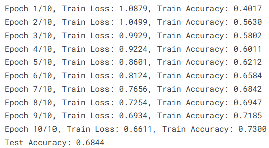
4.5模型评估
模型训练完成后,需要对模型的分类效果进行评估。首先利用分类报告(Classification Report)对模型的预测性能进行统计分析。分类报告主要包括精确率(Precision)、召回率(Recall)、F1值(F1-score)以及各类别样本数量等指标。其中,精确率反映模型预测为某一类别时的准确程度,召回率反映模型对该类别样本的识别能力,而F1值则综合考虑了精确率与召回率,是评价分类模型性能的重要指标。
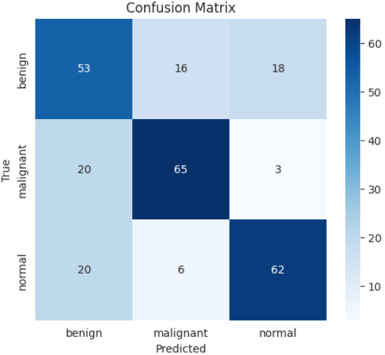
在此基础上,进一步通过混淆矩阵(Confusion Matrix)对模型的分类结果进行可视化分析。混淆矩阵以矩阵形式展示真实类别与预测类别之间的对应关系,通过观察矩阵中各元素的分布情况,可以直观地了解模型在哪些类别上预测效果较好,以及是否存在误分类现象。该方法能够帮助进一步分析模型在不同类别上的识别能力,为后续模型优化提供参考。
# =========================
# 输出分类报告
# =========================

print("\nClassification Report:")

# classification_report会输出每个类别的
# precision(精确率)、recall(召回率)、f1-score以及样本数量
print(classification_report(
    all_labels,              # 真实标签
    all_preds,               # 模型预测标签
    target_names=train_dataset.classes   # 类别名称
))


# =========================
# 计算混淆矩阵
# =========================

# confusion_matrix用于统计预测结果与真实结果之间的对应关系
cm = confusion_matrix(all_labels, all_preds)


# =========================
# 可视化混淆矩阵
# =========================

plt.figure(figsize=(6, 5))

# 使用seaborn绘制热力图形式的混淆矩阵
sns.heatmap(
    cm,
    annot=True,              # 显示具体数值
    fmt='d',                 # 以整数形式显示
    cmap="Blues",            # 颜色风格
    xticklabels=train_dataset.classes,   # x轴标签(预测类别)
    yticklabels=train_dataset.classes    # y轴标签(真实类别)
)

plt.xlabel("Predicted")      # x轴名称
plt.ylabel("True")           # y轴名称
plt.title("Confusion Matrix")# 图标题

plt.show()                   # 显示图像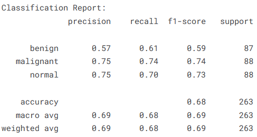
为了进一步分析模型在训练过程中的学习情况,本研究对训练阶段的损失变化和准确率变化进行了可视化展示。通过绘制训练损失曲线,可以观察模型在不同训练轮次中的损失变化趋势。如果损失值随着训练轮次逐渐下降,说明模型能够不断学习数据特征并逐步收敛。与此同时,通过绘制训练准确率曲线,可以直观地反映模型在训练集上的分类能力变化情况。当准确率随训练轮次逐步提升并趋于稳定时,表明模型已经较好地学习到了数据中的有效特征。
# =========================
# 可视化训练过程
# =========================

plt.figure(figsize=(10, 4))


# =========================
# 绘制训练损失曲线
# =========================

plt.subplot(1, 2, 1)  # 创建1行2列子图中的第1个图

# train_loss_history记录了每个epoch的损失值
plt.plot(train_loss_history, marker='o')

plt.title('Training Loss')   # 图标题
plt.xlabel('Epoch')          # x轴表示训练轮数
plt.ylabel('Loss')           # y轴表示损失值


# =========================
# 绘制训练准确率曲线
# =========================

plt.subplot(1, 2, 2)  # 创建第2个子图

# train_accuracy_history记录每个epoch的训练准确率
plt.plot(train_accuracy_history, marker='o')

plt.title('Training Accuracy')  # 图标题
plt.xlabel('Epoch')             # x轴表示训练轮数
plt.ylabel('Accuracy')          # y轴表示准确率


# 自动调整子图间距
plt.tight_layout()

# 显示图像
plt.show()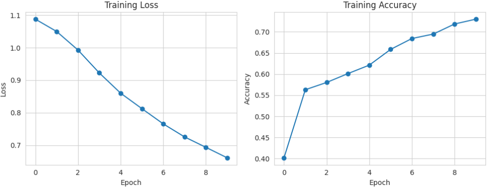
5.总结
本实验基于Kaggle公开的乳腺超声图像数据集,构建了一个结合Vision Transformer(ViT)与图神经网络(GNN)的乳腺超声图像分类模型,对正常、良性和恶性三类乳腺组织进行自动识别。实验过程中首先对数据集进行了整理与类别均衡处理,并完成了图像预处理与标准化操作,在此基础上利用ViT提取图像的深层视觉特征,再通过GNN对图像patch之间的结构关系进行建模,从而实现图像特征的进一步融合与表达。实验结果表明,该模型在测试集上取得了68.44%的整体分类准确率,其中恶性与正常样本的识别效果相对较好,而良性样本的识别性能略低。从分类报告可以看出,各类别的F1值整体维持在0.59至0.74之间,说明模型已经能够在一定程度上捕捉乳腺超声图像中的关键特征,但仍存在一定的提升空间。总体来看,ViT与GNN结合的建模思路在乳腺超声图像分类任务中具有一定可行性,为医学影像智能分析提供了一种新的研究思路,但在模型结构优化、数据规模扩展以及特征表达能力等方面仍有进一步改进的空间。
源代码
import numpy as np
import pandas as pd
import os
base_path = '/kaggle/input/breast-ultrasound-images-dataset/Dataset_BUSI_with_GT/'
tumor_types = ["benign", "malignant", "normal"]
image_paths = []
mask_paths = []
tumor_labels = []

for tumor in tumor_types:
    folder_path = os.path.join(base_path, tumor)

    if os.path.exists(folder_path):

        files = os.listdir(folder_path)

        image_files = [f for f in files if f.endswith(".png") and "_mask" not in f]

        for img_file in image_files:
            mask_file = img_file.replace(".png", "_mask.png")

            img_path = os.path.join(folder_path, img_file)
            mask_path = os.path.join(folder_path, mask_file)

            if os.path.exists(img_path) and os.path.exists(mask_path):
                image_paths.append(img_path)
                mask_paths.append(mask_path)
                tumor_labels.append(tumor)
            else:
                print(f"Missing pair for image: {img_path} or mask: {mask_path}")
    else:
        print(f"Folder not found: {folder_path}")

df = pd.DataFrame({
    "image_path": image_paths,
    "mask_path": mask_paths,
    "tumor_type": tumor_labels
})
df
import seaborn as sns
import matplotlib.pyplot as plt

sns.set_style("whitegrid")

fig, ax = plt.subplots(figsize=(8, 6))
sns.countplot(data=df, x="tumor_type", palette="viridis", ax=ax)

ax.set_title("Distribution of Disease Types", fontsize=14, fontweight='bold')
ax.set_xlabel("Tumor Type", fontsize=12)
ax.set_ylabel("Count", fontsize=12)

for p in ax.patches:
    ax.annotate(f'{int(p.get_height())}',
                (p.get_x() + p.get_width() / 2., p.get_height()),
                ha='center', va='bottom', fontsize=11, color='black',
                xytext=(0, 5), textcoords='offset points')

plt.show()
label_counts = df["tumor_type"].value_counts()

fig, ax = plt.subplots(figsize=(20, 8))
colors = sns.color_palette("viridis", len(label_counts))

ax.pie(label_counts, labels=label_counts.index, autopct='%1.1f%%',
       startangle=140, colors=colors, textprops={'fontsize': 12, 'weight': 'bold'},
       wedgeprops={'edgecolor': 'black', 'linewidth': 1})

ax.set_title("Distribution of Disease Types - Pie Chart", fontsize=14, fontweight='bold')

plt.show()
import matplotlib.pyplot as plt
import cv2

n_samples = 5
tumor_types = df['tumor_type'].unique()

for tumor in tumor_types:
    subset = df[df['tumor_type'] == tumor].sample(n=min(n_samples, len(df[df['tumor_type'] == tumor])), random_state=42)

    fig, axs = plt.subplots(2, n_samples, figsize=(3 * n_samples, 6))
    fig.suptitle(f"Tumor Type: {tumor}", fontsize=16)

    for i, (idx, row) in enumerate(subset.iterrows()):
        image = cv2.imread(row['image_path'], cv2.IMREAD_GRAYSCALE)
        mask = cv2.imread(row['mask_path'], cv2.IMREAD_GRAYSCALE)

        axs[0, i].imshow(image, cmap='gray')
        axs[0, i].axis('off')
        axs[0, i].set_title(f"Image {i+1}")

        axs[1, i].imshow(mask, cmap='gray')
        axs[1, i].axis('off')
        axs[1, i].set_title(f"Mask {i+1}")

    plt.tight_layout()
    plt.show()
df_benign = df[df["tumor_type"] == "benign"]
df_malignant = df[df["tumor_type"] == "malignant"]
df_normal = df[df["tumor_type"] == "normal"]
max_size = max(len(df_benign), len(df_malignant), len(df_normal))
from sklearn.utils import resample

df_malignant_oversampled = resample(df_malignant,
                                     replace=True,
                                     n_samples=max_size,
                                     random_state=42)
df_normal_oversampled = resample(df_normal,
                                    replace=True,
                                    n_samples=max_size,
                                    random_state=42)

df_balanced = pd.concat([df_benign, df_malignant_oversampled, df_normal_oversampled])
df_balanced = df_balanced.sample(frac=1, random_state=42).reset_index(drop=True)
df = df_balanced
df = df.drop(['mask_path'], axis = 1)
import torch
import torch.nn as nn
import torch.optim as optim
from torch.utils.data import Dataset, DataLoader
from torchvision import transforms
from PIL import Image
import pandas as pd
from sklearn.model_selection import train_test_split
from sklearn.preprocessing import LabelEncoder
from sklearn.metrics import confusion_matrix, classification_report
import seaborn as sns
import matplotlib.pyplot as plt
import numpy as np
from transformers import ViTModel, ViTFeatureExtractor
from torch_geometric.nn import GCNConv

IMAGE_SIZE = 224
BATCH_SIZE = 16
NUM_EPOCHS = 10
LEARNING_RATE = 1e-4
NUM_CLASSES = 3
VIT_MODEL_NAME = "google/vit-base-patch16-224-in21k"
PATCH_SIZE = 16
NUM_PATCHES = (IMAGE_SIZE // PATCH_SIZE) * (IMAGE_SIZE // PATCH_SIZE)
GNN_HIDDEN_DIM = 128

class BreastUltrasoundDataset(Dataset):
    def __init__(self, dataframe, transform=None):
        self.dataframe = dataframe
        self.transform = transform
        self.label_encoder = LabelEncoder()
        self.dataframe['tumor_type_encoded'] = self.label_encoder.fit_transform(self.dataframe['tumor_type'])
        self.classes = self.label_encoder.classes_

    def __len__(self):
        return len(self.dataframe)

    def __getitem__(self, idx):
        img_path = self.dataframe.iloc[idx]['image_path']
        image = Image.open(img_path).convert('RGB')
        label = self.dataframe.iloc[idx]['tumor_type_encoded']
        if self.transform:
            image = self.transform(image)
        return image, label

transform = transforms.Compose([
    transforms.Resize((IMAGE_SIZE, IMAGE_SIZE)),
    transforms.ToTensor(),
    transforms.Normalize(mean=[0.485, 0.456, 0.406], std=[0.229, 0.224, 0.225]),
])

class ViTGNNClassifier(nn.Module):
    def __init__(self, num_classes, vit_model_name=VIT_MODEL_NAME, gnn_hidden_dim=GNN_HIDDEN_DIM, patch_size=PATCH_SIZE):
        super(ViTGNNClassifier, self).__init__()
        self.vit = ViTModel.from_pretrained(vit_model_name)
        self.feature_extractor = ViTFeatureExtractor.from_pretrained(vit_model_name)
        for param in self.vit.parameters():
            param.requires_grad = False
        self.patch_size = patch_size
        self.num_patches = (IMAGE_SIZE // self.patch_size) * (IMAGE_SIZE // self.patch_size)
        self.vit_feature_dim = self.vit.config.hidden_size
        self.gcn1 = GCNConv(self.vit_feature_dim, gnn_hidden_dim)
        self.gcn2 = GCNConv(gnn_hidden_dim, gnn_hidden_dim)
        self.classifier = nn.Sequential(
            nn.Linear(gnn_hidden_dim, num_classes)
        )

    def forward(self, images):
        processed_images = []
        for i in range(images.shape[0]):
            img_tensor = images[i].cpu()
            img_np = img_tensor.permute(1, 2, 0).numpy()
            img_np = (img_np * 255).astype(np.uint8)
            processed_images.append(img_np)
        pixel_values = self.feature_extractor(processed_images, return_tensors="pt").pixel_values.to(images.device)
        vit_outputs = self.vit(pixel_values)
        patch_embeddings = vit_outputs.last_hidden_state[:, 1:]
        batch_size, num_patches, feature_dim = patch_embeddings.shape
        gnn_outputs = []
        for i in range(batch_size):
            features = patch_embeddings[i]
            edge_index = torch.combinations(torch.arange(num_patches), 2).t().contiguous().to(images.device)
            edge_index = torch.cat([edge_index, edge_index.flip(0)], dim=1)
            x = self.gcn1(features, edge_index)
            x = torch.relu(x)
            x = self.gcn2(x, edge_index)
            x = torch.relu(x)
            graph_embedding = torch.mean(x, dim=0)
            gnn_outputs.append(graph_embedding)
        combined_features = torch.stack(gnn_outputs, dim=0)
        logits = self.classifier(combined_features)
        return logits

train_df, test_df = train_test_split(df, test_size=0.2, random_state=42, stratify=df['tumor_type'])
train_dataset = BreastUltrasoundDataset(train_df, transform=transform)
test_dataset = BreastUltrasoundDataset(test_df, transform=transform)
train_loader = DataLoader(train_dataset, batch_size=BATCH_SIZE, shuffle=True)
test_loader = DataLoader(test_dataset, batch_size=BATCH_SIZE, shuffle=False)

device = torch.device("cuda" if torch.cuda.is_available() else "cpu")
model = ViTGNNClassifier(num_classes=NUM_CLASSES).to(device)
criterion = nn.CrossEntropyLoss()
optimizer = optim.AdamW(model.parameters(), lr=LEARNING_RATE)

train_loss_history = []
train_accuracy_history = []

for epoch in range(NUM_EPOCHS):
    model.train()
    running_loss = 0.0
    correct_predictions = 0
    total_predictions = 0
    for images, labels in train_loader:
        images, labels = images.to(device), labels.to(device)
        optimizer.zero_grad()
        outputs = model(images)
        loss = criterion(outputs, labels)
        loss.backward()
        optimizer.step()
        running_loss += loss.item() * images.size(0)
        _, predicted = torch.max(outputs.data, 1)
        total_predictions += labels.size(0)
        correct_predictions += (predicted == labels).sum().item()
    epoch_loss = running_loss / len(train_dataset)
    epoch_accuracy = correct_predictions / total_predictions
    train_loss_history.append(epoch_loss)
    train_accuracy_history.append(epoch_accuracy)
    print(f"Epoch {epoch+1}/{NUM_EPOCHS}, Train Loss: {epoch_loss:.4f}, Train Accuracy: {epoch_accuracy:.4f}")

model.eval()
test_correct_predictions = 0
test_total_predictions = 0
all_preds = []
all_labels = []

with torch.no_grad():
    for images, labels in test_loader:
        images, labels = images.to(device), labels.to(device)
        outputs = model(images)
        _, predicted = torch.max(outputs.data, 1)
        test_total_predictions += labels.size(0)
        test_correct_predictions += (predicted == labels).sum().item()
        all_preds.extend(predicted.cpu().numpy())
        all_labels.extend(labels.cpu().numpy())

test_accuracy = test_correct_predictions / test_total_predictions
print(f"Test Accuracy: {test_accuracy:.4f}")
print("\nClassification Report:")
print(classification_report(all_labels, all_preds, target_names=train_dataset.classes))

cm = confusion_matrix(all_labels, all_preds)
plt.figure(figsize=(6, 5))
sns.heatmap(cm, annot=True, fmt='d', cmap="Blues", xticklabels=train_dataset.classes, yticklabels=train_dataset.classes)
plt.xlabel("Predicted")
plt.ylabel("True")
plt.title("Confusion Matrix")
plt.show()
plt.figure(figsize=(10, 4))
plt.subplot(1, 2, 1)
plt.plot(train_loss_history, marker='o')
plt.title('Training Loss')
plt.xlabel('Epoch')
plt.ylabel('Loss')

plt.subplot(1, 2, 2)
plt.plot(train_accuracy_history, marker='o')
plt.title('Training Accuracy')
plt.xlabel('Epoch')
plt.ylabel('Accuracy')
plt.tight_layout()
plt.show()
资料获取,更多粉丝福利,关注下方公众号获取


AtomGit 是由开放原子开源基金会联合 CSDN 等生态伙伴共同推出的新一代开源与人工智能协作平台。平台坚持“开放、中立、公益”的理念,把代码托管、模型共享、数据集托管、智能体开发体验和算力服务整合在一起,为开发者提供从开发、训练到部署的一站式体验。
更多推荐
 32
32 0
0- 0


 已为社区贡献6条内容

所有评论(0)