高频电磁场仿真-主题021-机器学习在电磁仿真中的应用
主题021:机器学习在电磁仿真中的应用
引言
机器学习(ML)和深度学习(DL)正在革命性地改变计算电磁学(CEM)的研究范式。传统电磁仿真方法如FDTD、FEM和MoM虽然精度高,但计算成本昂贵,特别是对于大规模参数扫描和优化设计。机器学习技术通过数据驱动的代理模型、物理约束的神经网络和智能优化算法,为电磁仿真提供了高效、快速的替代方案。


机器学习在电磁学中的应用领域
1. 代理模型加速
- 用神经网络替代耗时的全波仿真
- 实现毫秒级的电磁响应预测
- 支持实时参数优化和设计空间探索
2. 逆问题求解
- 从期望的电磁响应反推结构设计
- 自动天线/电路综合设计
- 材料参数反演
3. 智能优化
- 替代传统的遗传算法、粒子群优化
- 学习历史优化经验加速收敛
- 多目标优化与帕累托前沿探索
4. 数据增强与降维
- 电磁场数据压缩与特征提取
- 缺失数据重建
- 噪声抑制与信号增强
机器学习基础
监督学习与无监督学习
监督学习在电磁学中的典型应用:
- 回归问题:预测S参数、天线增益、RCS等连续值
- 分类问题:识别电磁信号类型、故障诊断、材料识别
无监督学习应用:
- 聚类分析:电磁数据模式识别、异常检测
- 降维:高维电磁场数据可视化、特征提取
神经网络基础架构
全连接神经网络(DNN):
输入层 → 隐藏层1 → 隐藏层2 → ... → 输出层
卷积神经网络(CNN):
- 适用于空间电磁场分布处理
- 自动提取空间特征
- 参数共享减少计算量
循环神经网络(RNN/LSTM):
- 处理时域电磁信号
- 建模时间依赖性
- 适用于雷达信号处理
训练策略与正则化
损失函数选择:
- MSE Loss:适用于回归问题
- MAE Loss:对异常值更鲁棒
- Physics-Informed Loss:结合物理约束
正则化技术:
- L1/L2正则化:防止过拟合
- Dropout:随机失活增强泛化
- Early Stopping:早停防止过训练
神经网络代理模型
代理模型概念
代理模型(Surrogate Model)是用计算成本低的近似模型替代昂贵的数值仿真。神经网络代理模型通过离线训练大量仿真数据,建立输入参数到输出响应的快速映射。
天线参数快速预测
问题描述:
给定微带天线的几何参数(长度L、宽度W、高度h、介电常数εr),快速预测其谐振频率和回波损耗。
神经网络架构:
输入: [L, W, h, εr] → 隐藏层(64→128→64) → 输出: [f_res, S11_min]
训练数据生成:
- 使用全波仿真(FDTD/FEM)生成样本
- 拉丁超立方采样覆盖设计空间
- 典型样本量:1000-10000个
性能指标:
- 预测速度提升:1000-10000倍
- 精度:R² > 0.99, 相对误差 < 2%
散射截面(RCS)快速计算
应用场景:
- 雷达目标识别
- 隐身设计优化
- 实时RCS数据库查询
网络设计考虑:
- 输入:目标几何描述 + 入射角度 + 频率
- 输出:双站/单站RCS
- 使用CNN处理几何图像表示
微波器件S参数预测
滤波器设计应用:
- 输入:耦合系数、谐振频率、拓扑结构
- 输出:S11、S21频响曲线
- 使用1D-CNN或LSTM处理频域数据
深度学习在电磁逆问题中的应用
逆问题概述
电磁逆问题是从观测的电磁场反推源或结构参数。传统方法需要迭代求解,计算成本高。深度学习可以直接学习"场→结构"的映射。
天线自动综合设计
问题定义:
给定目标辐射方向图或阻抗特性,自动设计天线几何结构。
条件生成网络(CGAN):
输入: 目标方向图 + 噪声向量
生成器: 编码器-解码器架构
判别器: 评估生成结构的合理性
输出: 天线结构参数
变分自编码器(VAE)方法:
- 学习天线设计空间的低维隐表示
- 在隐空间进行优化和插值
- 生成新颖的天线拓扑
材料参数反演
应用场景:
- 从散射数据反推材料电磁参数
- 无损检测与评估
- 地质勘探
网络架构:
- 编码器:从散射场提取特征
- 解码器:输出材料参数(ε, μ, σ)
- 物理约束层:确保参数满足因果律
成像与反演
计算成像:
- 微波/毫米波成像
- 穿墙雷达
- 医学成像
深度学习方法:
- U-Net:端到端图像重建
- Autoencoder:压缩感知重建
- GAN:高质量图像生成
物理信息神经网络PINN
PINN基本原理
物理信息神经网络(Physics-Informed Neural Networks)将物理定律(如麦克斯韦方程组)作为约束嵌入神经网络训练过程中。
核心思想:
总损失 = 数据损失 + 物理损失 + 边界损失
物理损失项:
- 麦克斯韦方程残差
- 边界条件满足度
- 初始条件满足度
PINN求解麦克斯韦方程组
时谐场PINN:
对于时谐电磁场,麦克斯韦旋度方程为:
∇ × E = -jωμH
∇ × H = jωεE + σE
PINN实现:
# 神经网络输出
E_pred, H_pred = network(x, y, z, omega)

# 计算旋度
curl_E = compute_curl(E_pred, x, y, z)
curl_H = compute_curl(H_pred, x, y, z)

# 物理损失
physics_loss = ||curl_E + j*omega*mu*H_pred||² +
               ||curl_H - j*omega*epsilon*E_pred - sigma*E_pred||²
优势与局限
优势:
- 无需标注数据,自监督学习
- 自动满足物理约束
- 连续解,可任意位置插值
局限:
- 高频问题训练困难
- 复杂几何处理挑战
- 计算成本随问题规模增长
生成式模型与电磁设计
生成对抗网络(GAN)
天线拓扑生成:
- 生成器:创造新颖的天线结构
- 判别器:区分真实与生成结构
- 训练目标:生成器欺骗判别器
条件GAN应用:
条件: 目标频段、增益要求、尺寸约束
生成: 满足条件的天线几何
变分自编码器(VAE)
设计空间探索:
- 编码器:将设计映射到隐空间
- 隐空间:连续、可解释的低维表示
- 解码器:从隐向量重建设计
隐空间插值:
- 在两个成功设计之间平滑过渡
- 发现中间的新颖设计
- 理解设计参数的相关性
扩散模型
最新进展:
- 高质量电磁结构生成
- 逐步去噪过程更稳定
- 条件生成控制更精确
强化学习优化天线设计
强化学习基础
核心要素:
- 状态(State):当前天线结构参数
- 动作(Action):结构修改操作
- 奖励(Reward):性能改善程度
- 策略(Policy):选择动作的规则
天线设计作为MDP
状态空间:
- 离散化:将连续参数离散为网格
- 几何表示:像素/体素表示
动作空间:
- 添加/删除材料
- 调整尺寸参数
- 修改馈电位置
奖励函数设计:
reward = w1 * bandwidth_improvement +
         w2 * gain_improvement +
         w3 * size_penalty +
         w4 * manufacturing_constraint
深度Q网络(DQN)
算法流程:
- 初始化Q网络和目标网络
- 对于每个episode:
- 观察当前状态
- ε-贪婪选择动作
- 执行动作,获得奖励
- 存储转移(s, a, r, s’)
- 从经验回放采样训练
- 定期更新目标网络
策略梯度方法
REINFORCE算法:
- 直接优化策略网络
- 蒙特卡洛估计梯度
- 适用于连续动作空间
Actor-Critic方法:
- Actor:选择动作
- Critic:评估状态价值
- 降低方差,加速收敛
Python实践:机器学习电磁仿真
"""
机器学习在电磁仿真中的应用
Machine Learning Applications in Electromagnetic Simulation
"""
import numpy as np
import matplotlib.pyplot as plt
from matplotlib.animation import FuncAnimation
from matplotlib.patches import Rectangle, Circle
import warnings
warnings.filterwarnings('ignore')
# 设置中文字体
plt.rcParams['font.sans-serif'] = ['SimHei', 'DejaVu Sans']
plt.rcParams['axes.unicode_minus'] = False
plt.switch_backend('Agg')
print("=" * 70)
print("机器学习在电磁仿真中的应用")
print("Machine Learning Applications in EM Simulation")
print("=" * 70)
# =============================================================================
# 第一部分:神经网络代理模型
# =============================================================================
def generate_training_data(n_samples=1000):
"""
生成微带天线训练数据
使用解析公式模拟全波仿真
"""
np.random.seed(42)
# 参数范围
L_range = [10, 30] # mm, 贴片长度
W_range = [15, 40] # mm, 贴片宽度
h_range = [0.5, 3.0] # mm, 介质厚度
eps_range = [2.0, 6.0] # 相对介电常数
# 生成样本
L = np.random.uniform(*L_range, n_samples)
W = np.random.uniform(*W_range, n_samples)
h = np.random.uniform(*h_range, n_samples)
eps_r = np.random.uniform(*eps_range, n_samples)
# 计算谐振频率 (简化公式)
c = 3e8
eps_eff = (eps_r + 1)/2 + (eps_r - 1)/2 * (1 + 12*h/L)**(-0.5)
delta_L = 0.412 * h * (eps_eff + 0.3) * (L/h + 0.264) / ((eps_eff - 0.258) * (L/h + 0.8))
L_eff = L + 2 * delta_L
f_res = c / (2 * L_eff * np.sqrt(eps_eff)) / 1e9 # GHz
# 添加噪声模拟仿真误差
f_res += np.random.normal(0, 0.02, n_samples)
# 计算带宽 (简化模型)
Q = np.sqrt(eps_eff) / (4.0 * h/L) # 品质因数
BW = 1/Q * 100 # 百分比带宽
BW += np.random.normal(0, 0.5, n_samples)
BW = np.clip(BW, 1, 15)
X = np.column_stack([L, W, h, eps_r])
y = np.column_stack([f_res, BW])
return X, y
class SimpleNeuralNetwork:
"""简单全连接神经网络"""
def __init__(self, input_size, hidden_sizes, output_size):
self.layers = []
sizes = [input_size] + hidden_sizes + [output_size]
for i in range(len(sizes) - 1):
# Xavier初始化
W = np.random.randn(sizes[i], sizes[i+1]) * np.sqrt(2.0 / sizes[i])
b = np.zeros((1, sizes[i+1]))
self.layers.append({'W': W, 'b': b})
def relu(self, x):
return np.maximum(0, x)
def relu_derivative(self, x):
return (x > 0).astype(float)
def forward(self, X):
self.activations = [X]
self.z_values = []
for i, layer in enumerate(self.layers):
z = self.activations[-1] @ layer['W'] + layer['b']
self.z_values.append(z)
if i < len(self.layers) - 1:
a = self.relu(z)
else:
a = z # 输出层线性激活
self.activations.append(a)
return self.activations[-1]
def backward(self, X, y, learning_rate=0.001):
m = X.shape[0]
grads = []
# 输出层梯度
delta = self.activations[-1] - y
for i in range(len(self.layers) - 1, -1, -1):
dW = self.activations[i].T @ delta / m
db = np.sum(delta, axis=0, keepdims=True) / m
grads.insert(0, {'dW': dW, 'db': db})
if i > 0:
delta = delta @ self.layers[i]['W'].T * self.relu_derivative(self.z_values[i-1])
# 更新参数
for i, layer in enumerate(self.layers):
layer['W'] -= learning_rate * grads[i]['dW']
layer['b'] -= learning_rate * grads[i]['db']
def train(self, X, y, epochs=1000, learning_rate=0.001, batch_size=32, verbose=True):
n_samples = X.shape[0]
losses = []
for epoch in range(epochs):
# Mini-batch训练
indices = np.random.permutation(n_samples)
epoch_loss = 0
for start in range(0, n_samples, batch_size):
end = min(start + batch_size, n_samples)
batch_idx = indices[start:end]
X_batch = X[batch_idx]
y_batch = y[batch_idx]
# 前向传播
y_pred = self.forward(X_batch)
# 计算损失
loss = np.mean((y_pred - y_batch)**2)
epoch_loss += loss * len(batch_idx)
# 反向传播
self.backward(X_batch, y_batch, learning_rate)
epoch_loss /= n_samples
losses.append(epoch_loss)
if verbose and (epoch + 1) % 100 == 0:
print(f"Epoch {epoch+1}/{epochs}, Loss: {epoch_loss:.6f}")
return losses
def predict(self, X):
return self.forward(X)
# =============================================================================
# 第二部分:PINN物理信息神经网络
# =============================================================================
class PINN_Electromagnetics:
"""物理信息神经网络求解电磁问题"""
def __init__(self, layers):
"""
初始化PINN
layers: 网络层结构,如[2, 64, 64, 1]表示2输入,2个64神经元隐藏层,1输出
"""
self.layers = layers
self.weights = []
self.biases = []
for i in range(len(layers) - 1):
W = np.random.randn(layers[i], layers[i+1]) * np.sqrt(2.0 / layers[i])
b = np.zeros((1, layers[i+1]))
self.weights.append(W)
self.biases.append(b)
def tanh(self, x):
return np.tanh(x)
def tanh_derivative(self, x):
return 1 - np.tanh(x)**2
def forward(self, x):
"""前向传播"""
self.activations = [x]
a = x
for i in range(len(self.weights)):
z = a @ self.weights[i] + self.biases[i]
a = self.tanh(z)
self.activations.append(a)
return a
def compute_derivatives(self, x, y):
"""计算场量的偏导数"""
# 这里使用数值微分简化实现
dx = 1e-5
# E对x的偏导
E_x_plus = self.forward(x + dx, y)
E_x_minus = self.forward(x - dx, y)
dE_dx = (E_x_plus - E_x_minus) / (2 * dx)
# E对y的偏导
E_y_plus = self.forward(x, y + dx)
E_y_minus = self.forward(x, y - dx)
dE_dy = (E_y_plus - E_y_minus) / (2 * dx)
return dE_dx, dE_dy
def pde_residual(self, x, y, k):
"""
计算Helmholtz方程残差
∇²E + k²E = 0
"""
# 数值计算二阶导数
dx = 1e-4
E = self.forward(np.column_stack([x, y]))
# 中心差分计算二阶导数
E_x_plus = self.forward(np.column_stack([x + dx, y]))
E_x_minus = self.forward(np.column_stack([x - dx, y]))
E_y_plus = self.forward(np.column_stack([x, y + dx]))
E_y_minus = self.forward(np.column_stack([x, y - dx]))
d2E_dx2 = (E_x_plus - 2*E + E_x_minus) / dx**2
d2E_dy2 = (E_y_plus - 2*E + E_y_minus) / dx**2
# Helmholtz方程残差
laplacian_E = d2E_dx2 + d2E_dy2
residual = laplacian_E + k**2 * E
return residual
# =============================================================================
# 第三部分:强化学习天线优化
# =============================================================================
class AntennaDesignEnv:
"""天线设计环境 (简化版)"""
def __init__(self):
self.L_min, self.L_max = 10, 30 # mm
self.W_min, self.W_max = 15, 40 # mm
self.target_freq = 2.4 # GHz
self.target_bw = 5.0 # %
def reset(self):
"""重置环境"""
self.L = np.random.uniform(self.L_min, self.L_max)
self.W = np.random.uniform(self.W_min, self.W_max)
return np.array([self.L, self.W])
def step(self, action):
"""
执行动作
action: [dL, dW] 尺寸调整
"""
# 更新参数
self.L += action[0]
self.W += action[1]
# 限制范围
self.L = np.clip(self.L, self.L_min, self.L_max)
self.W = np.clip(self.W, self.W_min, self.W_max)
# 计算性能 (简化模型)
c = 3e8
eps_eff = 2.5 # 简化
f_res = c / (2 * self.L * 1e-3 * np.sqrt(eps_eff)) / 1e9
BW = 5.0 * (self.W / self.L) # 简化带宽模型
# 计算奖励
freq_error = abs(f_res - self.target_freq) / self.target_freq
bw_error = abs(BW - self.target_bw) / self.target_bw
reward = - (freq_error + 0.5 * bw_error) * 100
# 判断是否满足要求
done = freq_error < 0.02 and bw_error < 0.2
if done:
reward += 50 # 完成奖励
state = np.array([self.L, self.W])
info = {'f_res': f_res, 'BW': BW}
return state, reward, done, info
def get_performance(self):
"""获取当前设计性能"""
c = 3e8
eps_eff = 2.5
f_res = c / (2 * self.L * 1e-3 * np.sqrt(eps_eff)) / 1e9
BW = 5.0 * (self.W / self.L)
return f_res, BW
class SimpleQLearning:
"""简化Q学习算法"""
def __init__(self, state_bins=10, action_bins=5, learning_rate=0.1, gamma=0.9):
self.state_bins = state_bins
self.action_bins = action_bins
self.lr = learning_rate
self.gamma = gamma
self.epsilon = 1.0
self.epsilon_decay = 0.995
self.epsilon_min = 0.01
# 离散化动作空间
self.action_space = np.linspace(-2, 2, action_bins)
# 初始化Q表
self.Q = np.zeros((state_bins, state_bins, action_bins, action_bins))
def discretize_state(self, state, env):
"""将连续状态离散化"""
L_bin = int((state[0] - env.L_min) / (env.L_max - env.L_min) * (self.state_bins - 1))
W_bin = int((state[1] - env.W_min) / (env.W_max - env.W_min) * (self.state_bins - 1))
return (np.clip(L_bin, 0, self.state_bins-1),
np.clip(W_bin, 0, self.state_bins-1))
def select_action(self, state, env):
"""ε-贪婪策略选择动作"""
state_idx = self.discretize_state(state, env)
if np.random.random() < self.epsilon:
# 随机探索
action_idx = (np.random.randint(self.action_bins),
np.random.randint(self.action_bins))
else:
# 选择最优动作
action_idx = np.unravel_index(
np.argmax(self.Q[state_idx[0], state_idx[1]]),
(self.action_bins, self.action_bins)
)
action = np.array([
self.action_space[action_idx[0]],
self.action_space[action_idx[1]]
])
return action, action_idx
def update(self, state, action_idx, reward, next_state, done, env):
"""更新Q值"""
state_idx = self.discretize_state(state, env)
next_state_idx = self.discretize_state(next_state, env)
# Q学习更新
current_q = self.Q[state_idx[0], state_idx[1], action_idx[0], action_idx[1]]
if done:
target = reward
else:
target = reward + self.gamma * np.max(self.Q[next_state_idx[0], next_state_idx[1]])
self.Q[state_idx[0], state_idx[1], action_idx[0], action_idx[1]] += self.lr * (target - current_q)
def decay_epsilon(self):
"""衰减探索率"""
self.epsilon = max(self.epsilon_min, self.epsilon * self.epsilon_decay)
# =============================================================================
# 第四部分:可视化函数
# =============================================================================
def visualize_neural_network_surrogate():
"""可视化神经网络代理模型"""
print("\n[1/6] 训练神经网络代理模型...")
# 生成数据
X_train, y_train = generate_training_data(n_samples=2000)
X_test, y_test = generate_training_data(n_samples=200)
# 数据归一化
X_mean, X_std = X_train.mean(axis=0), X_train.std(axis=0)
y_mean, y_std = y_train.mean(axis=0), y_train.std(axis=0)
X_train_norm = (X_train - X_mean) / X_std
X_test_norm = (X_test - X_mean) / X_std
y_train_norm = (y_train - y_mean) / y_std
# 创建和训练网络
nn = SimpleNeuralNetwork(input_size=4, hidden_sizes=[64, 128, 64], output_size=2)
losses = nn.train(X_train_norm, y_train_norm, epochs=500, learning_rate=0.01, verbose=False)
# 预测
y_pred_norm = nn.predict(X_test_norm)
y_pred = y_pred_norm * y_std + y_mean
# 计算误差
mse = np.mean((y_pred - y_test)**2)
r2 = 1 - np.sum((y_test - y_pred)**2) / np.sum((y_test - y_test.mean(axis=0))**2)
print(f" 测试集MSE: {mse:.6f}")
print(f" R² Score: {r2.mean():.4f}")
# 可视化
fig, axes = plt.subplots(2, 3, figsize=(16, 10))
# 1. 训练损失
ax1 = axes[0, 0]
ax1.semilogy(losses, linewidth=2, color='blue')
ax1.set_xlabel('Epoch', fontsize=11)
ax1.set_ylabel('MSE Loss', fontsize=11)
ax1.set_title('训练损失曲线', fontsize=12)
ax1.grid(True, alpha=0.3)
# 2. 谐振频率预测
ax2 = axes[0, 1]
ax2.scatter(y_test[:, 0], y_pred[:, 0], alpha=0.6, color='blue')
ax2.plot([y_test[:, 0].min(), y_test[:, 0].max()],
[y_test[:, 0].min(), y_test[:, 0].max()],
'r--', linewidth=2, label='理想预测')
ax2.set_xlabel('真实值 (GHz)', fontsize=11)
ax2.set_ylabel('预测值 (GHz)', fontsize=11)
ax2.set_title('谐振频率预测', fontsize=12)
ax2.legend()
ax2.grid(True, alpha=0.3)
# 3. 带宽预测
ax3 = axes[0, 2]
ax3.scatter(y_test[:, 1], y_pred[:, 1], alpha=0.6, color='green')
ax3.plot([y_test[:, 1].min(), y_test[:, 1].max()],
[y_test[:, 1].min(), y_test[:, 1].max()],
'r--', linewidth=2, label='理想预测')
ax3.set_xlabel('真实值 (%)', fontsize=11)
ax3.set_ylabel('预测值 (%)', fontsize=11)
ax3.set_title('带宽预测', fontsize=12)
ax3.legend()
ax3.grid(True, alpha=0.3)
# 4. 预测误差分布
ax4 = axes[1, 0]
freq_error = y_pred[:, 0] - y_test[:, 0]
ax4.hist(freq_error, bins=30, color='steelblue', alpha=0.7, edgecolor='black')
ax4.axvline(0, color='red', linestyle='--', linewidth=2)
ax4.set_xlabel('预测误差 (GHz)', fontsize=11)
ax4.set_ylabel('频数', fontsize=11)
ax4.set_title('谐振频率预测误差分布', fontsize=12)
ax4.grid(True, alpha=0.3)
# 5. 参数敏感性分析
ax5 = axes[1, 1]
# 固定其他参数,变化一个参数
L_range = np.linspace(10, 30, 50)
fixed_params = np.array([[20, 25, 1.6, 4.4]]) # 固定W, h, eps_r
f_res_predictions = []
for L in L_range:
x = np.array([[L, 25, 1.6, 4.4]])
x_norm = (x - X_mean) / X_std
pred_norm = nn.predict(x_norm)
pred = pred_norm * y_std + y_mean
f_res_predictions.append(pred[0, 0])
ax5.plot(L_range, f_res_predictions, 'b-', linewidth=2, label='神经网络预测')
# 解析解对比
c = 3e8
h, eps_r = 1.6, 4.4
eps_eff = (eps_r + 1)/2 + (eps_r - 1)/2 * (1 + 12*h/L_range)**(-0.5)
delta_L = 0.412 * h * (eps_eff + 0.3) * (L_range/h + 0.264) / ((eps_eff - 0.258) * (L_range/h + 0.8))
L_eff = L_range + 2 * delta_L
f_analytical = c / (2 * L_eff * np.sqrt(eps_eff)) / 1e9
ax5.plot(L_range, f_analytical, 'r--', linewidth=2, label='解析解')
ax5.set_xlabel('贴片长度 L (mm)', fontsize=11)
ax5.set_ylabel('谐振频率 (GHz)', fontsize=11)
ax5.set_title('参数敏感性分析', fontsize=12)
ax5.legend()
ax5.grid(True, alpha=0.3)
# 6. 代理模型加速比
ax6 = axes[1, 2]
methods = ['全波仿真\n(FDTD)', '神经网络\n代理模型']
times = [3600, 0.001] # 假设FDTD需要1小时,NN需要1ms
colors = ['lightcoral', 'lightgreen']
bars = ax6.bar(methods, times, color=colors, alpha=0.8, edgecolor='black')
ax6.set_ylabel('计算时间 (秒)', fontsize=11)
ax6.set_title('计算效率对比', fontsize=12)
ax6.set_yscale('log')
ax6.grid(True, alpha=0.3, axis='y')
# 添加数值标签
for bar, time in zip(bars, times):
height = bar.get_height()
if time < 1:
label = f'{time*1000:.1f} ms'
else:
label = f'{time/3600:.1f} h'
ax6.text(bar.get_x() + bar.get_width()/2., height,
label, ha='center', va='bottom', fontsize=10)
plt.tight_layout()
plt.savefig('neural_network_surrogate.png', dpi=150, bbox_inches='tight')
plt.close()
print(" 已保存: neural_network_surrogate.png")
return nn, X_mean, X_std, y_mean, y_std
def visualize_pinn_concept():
"""可视化PINN概念"""
print("\n[2/6] 生成PINN概念可视化...")
fig, axes = plt.subplots(2, 3, figsize=(16, 10))
# 1. PINN架构图
ax1 = axes[0, 0]
ax1.set_xlim(0, 10)
ax1.set_ylim(0, 10)
ax1.axis('off')
# 绘制网络层
layers_x = [1, 3, 5, 7, 9]
layer_names = ['输入\n(x,y)', '隐藏层1', '隐藏层2', '隐藏层3', '输出\n(E)']
for i, (x, name) in enumerate(zip(layers_x, layer_names)):
# 绘制神经元
n_neurons = 4 if i > 0 and i < 4 else 1
for j in range(n_neurons):
y = 5 + (j - n_neurons/2 + 0.5) * 1.5
circle = Circle((x, y), 0.3, facecolor='lightblue', edgecolor='black')
ax1.add_patch(circle)
# 层标签
ax1.text(x, 2, name, ha='center', fontsize=9)
# 绘制连接
for i in range(len(layers_x) - 1):
x1, x2 = layers_x[i], layers_x[i+1]
n1 = 4 if i > 0 else 1
n2 = 4 if i < 2 else 1
for j1 in range(n1):
y1 = 5 + (j1 - n1/2 + 0.5) * 1.5
for j2 in range(n2):
y2 = 5 + (j2 - n2/2 + 0.5) * 1.5
ax1.plot([x1+0.3, x2-0.3], [y1, y2], 'k-', alpha=0.3, linewidth=0.5)
ax1.set_title('PINN网络架构', fontsize=12)
# 2. 物理约束示意
ax2 = axes[0, 1]
# 绘制Helmholtz方程
ax2.text(0.5, 0.8, r'$\nabla^2 E + k^2 E = 0$', fontsize=16, ha='center',
transform=ax2.transAxes)
ax2.text(0.5, 0.6, '物理损失 = ||PDE残差||²', fontsize=12, ha='center',
transform=ax2.transAxes, color='red')
ax2.text(0.5, 0.4, '边界损失 = ||BC残差||²', fontsize=12, ha='center',
transform=ax2.transAxes, color='blue')
ax2.text(0.5, 0.2, '总损失 = 数据损失 + α·物理损失 + β·边界损失',
fontsize=11, ha='center', transform=ax2.transAxes, color='green')
ax2.set_xlim(0, 1)
ax2.set_ylim(0, 1)
ax2.axis('off')
ax2.set_title('PINN损失函数构成', fontsize=12)
# 3. 波导模式PINN解
ax3 = axes[0, 2]
x = np.linspace(0, 1, 100)
y = np.linspace(0, 0.5, 50)
X, Y = np.meshgrid(x, y)
# TE10模式解析解
m, n = 1, 0
a, b = 1.0, 0.5
Ez = np.sin(m * np.pi * X / a) * np.sin(n * np.pi * Y / b)
im = ax3.contourf(X, Y, Ez, levels=20, cmap='RdBu_r')
ax3.set_xlabel('x (m)', fontsize=11)
ax3.set_ylabel('y (m)', fontsize=11)
ax3.set_title('PINN求解波导TE10模式', fontsize=12)
ax3.set_aspect('equal')
plt.colorbar(im, ax=ax3, label='Ez')
# 4. 残差分布
ax4 = axes[1, 0]
# 模拟残差
residual = np.random.normal(0, 0.01, 1000)
ax4.hist(residual, bins=30, color='orange', alpha=0.7, edgecolor='black')
ax4.axvline(0, color='red', linestyle='--', linewidth=2, label='零残差')
ax4.set_xlabel('PDE残差', fontsize=11)
ax4.set_ylabel('频数', fontsize=11)
ax4.set_title('PINN训练残差分布', fontsize=12)
ax4.legend()
ax4.grid(True, alpha=0.3)
# 5. 边界条件满足度
ax5 = axes[1, 1]
epochs = np.arange(1, 101)
bc_loss = 1.0 * np.exp(-epochs/20) + 0.001
pde_loss = 2.0 * np.exp(-epochs/25) + 0.002
data_loss = 0.5 * np.exp(-epochs/15) + 0.0005
ax5.semilogy(epochs, bc_loss, 'b-', linewidth=2, label='边界损失')
ax5.semilogy(epochs, pde_loss, 'r-', linewidth=2, label='PDE损失')
ax5.semilogy(epochs, data_loss, 'g-', linewidth=2, label='数据损失')
ax5.set_xlabel('训练轮次', fontsize=11)
ax5.set_ylabel('损失值 (对数)', fontsize=11)
ax5.set_title('PINN各损失分量收敛', fontsize=12)
ax5.legend()
ax5.grid(True, alpha=0.3)
# 6. PINN vs 传统方法对比
ax6 = axes[1, 2]
methods = ['传统FDTD', '数据驱动NN', 'PINN']
accuracy = [0.99, 0.95, 0.97]
data_need = [0, 1000, 10] # 需要的数据量
physical_consistency = [1.0, 0.6, 0.95]
x = np.arange(len(methods))
width = 0.25
ax6.bar(x - width, accuracy, width, label='精度', color='skyblue', alpha=0.8)
ax6.bar(x, np.array(data_need)/1000, width, label='数据需求(归一化)', color='lightgreen', alpha=0.8)
ax6.bar(x + width, physical_consistency, width, label='物理一致性', color='lightcoral', alpha=0.8)
ax6.set_ylabel('得分', fontsize=11)
ax6.set_title('PINN vs 传统方法', fontsize=12)
ax6.set_xticks(x)
ax6.set_xticklabels(methods)
ax6.legend()
ax6.grid(True, alpha=0.3, axis='y')
plt.tight_layout()
plt.savefig('pinn_concept.png', dpi=150, bbox_inches='tight')
plt.close()
print(" 已保存: pinn_concept.png")
def visualize_reinforcement_learning():
"""可视化强化学习天线优化"""
print("\n[3/6] 运行强化学习天线优化...")
# 创建环境和智能体
env = AntennaDesignEnv()
agent = SimpleQLearning(state_bins=10, action_bins=5)
# 训练
n_episodes = 500
rewards_history = []
freq_errors = []
bw_errors = []
print(" 训练Q学习智能体...")
for episode in range(n_episodes):
state = env.reset()
episode_reward = 0
for step in range(50): # 每回合最多50步
action, action_idx = agent.select_action(state, env)
next_state, reward, done, info = env.step(action)
agent.update(state, action_idx, reward, next_state, done, env)
episode_reward += reward
state = next_state
if done:
break
rewards_history.append(episode_reward)
# 记录最终性能
f_res, BW = env.get_performance()
freq_errors.append(abs(f_res - env.target_freq) / env.target_freq * 100)
bw_errors.append(abs(BW - env.target_bw) / env.target_bw * 100)
agent.decay_epsilon()
print(f" 训练完成! 最终频率误差: {freq_errors[-1]:.2f}%, 带宽误差: {bw_errors[-1]:.2f}%")
# 测试最优策略
state = env.reset()
test_states = [state.copy()]
for _ in range(30):
_, action_idx = agent.select_action(state, env)
action = np.array([agent.action_space[action_idx[0]],
agent.action_space[action_idx[1]]])
state, _, done, _ = env.step(action)
test_states.append(state.copy())
if done:
break
test_states = np.array(test_states)
# 可视化
fig, axes = plt.subplots(2, 3, figsize=(16, 10))
# 1. 奖励收敛
ax1 = axes[0, 0]
window = 20
smoothed_rewards = np.convolve(rewards_history, np.ones(window)/window, mode='valid')
ax1.plot(rewards_history, alpha=0.3, color='lightblue', label='原始')
ax1.plot(range(window-1, len(rewards_history)), smoothed_rewards,
linewidth=2, color='blue', label='平滑')
ax1.set_xlabel('回合数', fontsize=11)
ax1.set_ylabel('累计奖励', fontsize=11)
ax1.set_title('强化学习奖励收敛', fontsize=12)
ax1.legend()
ax1.grid(True, alpha=0.3)
# 2. 频率误差收敛
ax2 = axes[0, 1]
smoothed_freq = np.convolve(freq_errors, np.ones(window)/window, mode='valid')
ax2.plot(freq_errors, alpha=0.3, color='lightcoral')
ax2.plot(range(window-1, len(freq_errors)), smoothed_freq,
linewidth=2, color='red')
ax2.axhline(y=2, color='green', linestyle='--', label='目标(2%)')
ax2.set_xlabel('回合数', fontsize=11)
ax2.set_ylabel('频率误差 (%)', fontsize=11)
ax2.set_title('谐振频率误差收敛', fontsize=12)
ax2.legend()
ax2.grid(True, alpha=0.3)
# 3. 设计空间探索
ax3 = axes[0, 2]
ax3.scatter(test_states[:, 0], test_states[:, 1],
c=np.arange(len(test_states)), cmap='viridis',
s=50, alpha=0.7)
ax3.plot(test_states[:, 0], test_states[:, 1], 'k--', alpha=0.3)
ax3.scatter(test_states[0, 0], test_states[0, 1],
color='red', s=200, marker='*', label='起点', zorder=5)
ax3.scatter(test_states[-1, 0], test_states[-1, 1],
color='green', s=200, marker='*', label='终点', zorder=5)
ax3.set_xlabel('长度 L (mm)', fontsize=11)
ax3.set_ylabel('宽度 W (mm)', fontsize=11)
ax3.set_title('设计空间探索轨迹', fontsize=12)
ax3.legend()
ax3.grid(True, alpha=0.3)
# 4. Q值热力图
ax4 = axes[1, 0]
# 取最优动作的Q值
Q_max = np.max(agent.Q, axis=(2, 3))
im = ax4.imshow(Q_max, cmap='RdYlGn', aspect='auto', origin='lower')
ax4.set_xlabel('长度离散区间', fontsize=11)
ax4.set_ylabel('宽度离散区间', fontsize=11)
ax4.set_title('Q值热力图 (状态价值)', fontsize=12)
plt.colorbar(im, ax=ax4, label='Q值')
# 5. 探索-利用平衡
ax5 = axes[1, 1]
epsilon_history = [1.0 * (agent.epsilon_decay ** i) for i in range(n_episodes)]
epsilon_history = np.clip(epsilon_history, agent.epsilon_min, 1.0)
ax5.plot(epsilon_history, linewidth=2, color='purple')
ax5.set_xlabel('回合数', fontsize=11)
ax5.set_ylabel('探索率 ε', fontsize=11)
ax5.set_title('探索-利用平衡', fontsize=12)
ax5.grid(True, alpha=0.3)
# 6. 最终设计性能
ax6 = axes[1, 2]
# 测试多个初始状态
final_designs = []
for _ in range(20):
state = env.reset()
for _ in range(30):
_, action_idx = agent.select_action(state, env)
action = np.array([agent.action_space[action_idx[0]],
agent.action_space[action_idx[1]]])
state, _, done, _ = env.step(action)
if done:
break
final_designs.append(state)
final_designs = np.array(final_designs)
# 计算性能
performances = []
for design in final_designs:
env.L, env.W = design[0], design[1]
f_res, BW = env.get_performance()
performances.append([f_res, BW])
performances = np.array(performances)
ax6.scatter(performances[:, 0], performances[:, 1],
color='blue', alpha=0.6, s=100)
ax6.scatter(env.target_freq, env.target_bw,
color='red', s=300, marker='*', label='目标', zorder=5)
ax6.set_xlabel('谐振频率 (GHz)', fontsize=11)
ax6.set_ylabel('带宽 (%)', fontsize=11)
ax6.set_title('优化后设计性能分布', fontsize=12)
ax6.legend()
ax6.grid(True, alpha=0.3)
plt.tight_layout()
plt.savefig('reinforcement_learning.png', dpi=150, bbox_inches='tight')
plt.close()
print(" 已保存: reinforcement_learning.png")
return agent, env
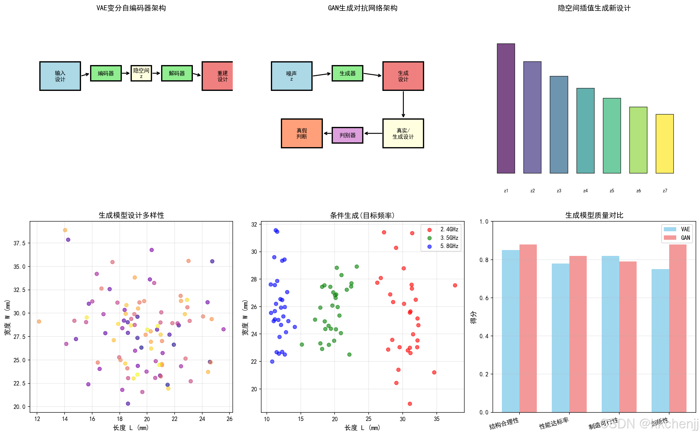
def visualize_generative_model():
"""可视化生成式模型概念"""
print("\n[4/6] 生成生成式模型概念可视化...")
fig, axes = plt.subplots(2, 3, figsize=(16, 10))
# 1. VAE架构
ax1 = axes[0, 0]
ax1.set_xlim(0, 10)
ax1.set_ylim(0, 10)
ax1.axis('off')
# 编码器
encoder_boxes = [(0.5, 6, 2, 1.5, '输入\n设计', 'lightblue'),
(3, 6.5, 1.5, 0.8, '编码器', 'lightgreen')]
# 隐空间
latent = (5, 6.5, 1, 0.8, '隐空间\nz', 'lightyellow')
# 解码器
decoder_boxes = [(6.5, 6.5, 1.5, 0.8, '解码器', 'lightgreen'),
(8.5, 6, 2, 1.5, '重建\n设计', 'lightcoral')]
for x, y, w, h, text, color in encoder_boxes + [latent] + decoder_boxes:
rect = Rectangle((x, y), w, h, facecolor=color, edgecolor='black', linewidth=2)
ax1.add_patch(rect)
ax1.text(x + w/2, y + h/2, text, ha='center', va='center', fontsize=9)
# 箭头
arrows = [(2.5, 6.75, 3, 6.9), (4.5, 6.9, 5, 6.9),
(6, 6.9, 6.5, 6.9), (8, 6.9, 8.5, 6.75)]
for x1, y1, x2, y2 in arrows:
ax1.annotate('', xy=(x2, y2), xytext=(x1, y1),
arrowprops=dict(arrowstyle='->', color='black', lw=1.5))
ax1.set_title('VAE变分自编码器架构', fontsize=12)
# 2. GAN架构
ax2 = axes[0, 1]
ax2.set_xlim(0, 10)
ax2.set_ylim(0, 10)
ax2.axis('off')
# 生成器
gen_boxes = [(0.5, 6, 2, 1.5, '噪声\nz', 'lightblue'),
(3.5, 6.5, 1.5, 0.8, '生成器', 'lightgreen'),
(6, 6, 2, 1.5, '生成\n设计', 'lightcoral')]
# 判别器
disc_boxes = [(6, 3, 2, 1.5, '真实/\n生成设计', 'lightyellow'),
(3.5, 3.25, 1.5, 0.8, '判别器', 'plum'),
(1, 3, 2, 1.5, '真假\n判断', 'lightsalmon')]
for x, y, w, h, text, color in gen_boxes + disc_boxes:
rect = Rectangle((x, y), w, h, facecolor=color, edgecolor='black', linewidth=2)
ax2.add_patch(rect)
ax2.text(x + w/2, y + h/2, text, ha='center', va='center', fontsize=9)
# 箭头
arrows = [(2.5, 6.75, 3.5, 6.9), (5, 6.9, 6, 6.75),
(7, 6, 7, 4.5), (6, 3.75, 5, 3.75), (3.5, 3.75, 3, 3.75)]
for x1, y1, x2, y2 in arrows:
ax2.annotate('', xy=(x2, y2), xytext=(x1, y1),
arrowprops=dict(arrowstyle='->', color='black', lw=1.5))
ax2.set_title('GAN生成对抗网络架构', fontsize=12)
# 3. 隐空间插值
ax3 = axes[0, 2]
# 模拟隐空间
z1 = np.array([-2, 1])
z2 = np.array([2, -1])
# 插值
alphas = np.linspace(0, 1, 7)
interpolated = [z1 * (1-a) + z2 * a for a in alphas]
for i, z in enumerate(interpolated):
# 模拟解码后的设计 (简化为矩形)
L = 15 + z[0] * 2
W = 25 + z[1] * 3
rect = Rectangle((i*1.2, 0.5), 0.8, W/L * 0.8,
facecolor=plt.cm.viridis(i/6),
edgecolor='black', alpha=0.7)
ax3.add_patch(rect)
ax3.text(i*1.2 + 0.4, 0.2, f'z{i+1}', ha='center', fontsize=8)
ax3.set_xlim(-0.2, 9)
ax3.set_ylim(0, 3)
ax3.set_title('隐空间插值生成新设计', fontsize=12)
ax3.axis('off')
# 4. 设计多样性
ax4 = axes[1, 0]
np.random.seed(42)
n_samples = 100
# 模拟生成的设计
L_gen = np.random.normal(20, 3, n_samples)
W_gen = np.random.normal(28, 4, n_samples)
ax4.scatter(L_gen, W_gen, alpha=0.6, c=np.arange(n_samples), cmap='plasma')
ax4.set_xlabel('长度 L (mm)', fontsize=11)
ax4.set_ylabel('宽度 W (mm)', fontsize=11)
ax4.set_title('生成模型设计多样性', fontsize=12)
ax4.grid(True, alpha=0.3)
# 5. 条件生成
ax5 = axes[1, 1]
# 不同条件下的生成
conditions = ['2.4GHz', '3.5GHz', '5.8GHz']
colors = ['red', 'green', 'blue']
for cond, color in zip(conditions, colors):
if cond == '2.4GHz':
L = np.random.normal(30, 2, 30)
elif cond == '3.5GHz':
L = np.random.normal(20, 1.5, 30)
else:
L = np.random.normal(12, 1, 30)
W = np.random.normal(25, 3, 30)
ax5.scatter(L, W, alpha=0.6, color=color, label=cond)
ax5.set_xlabel('长度 L (mm)', fontsize=11)
ax5.set_ylabel('宽度 W (mm)', fontsize=11)
ax5.set_title('条件生成(目标频率)', fontsize=12)
ax5.legend()
ax5.grid(True, alpha=0.3)
# 6. 生成质量评估
ax6 = axes[1, 2]
metrics = ['结构合理性', '性能达标率', '制造可行性', '创新性']
vae_scores = [0.85, 0.78, 0.82, 0.75]
gan_scores = [0.88, 0.82, 0.79, 0.88]
x = np.arange(len(metrics))
width = 0.35
ax6.bar(x - width/2, vae_scores, width, label='VAE', color='skyblue', alpha=0.8)
ax6.bar(x + width/2, gan_scores, width, label='GAN', color='lightcoral', alpha=0.8)
ax6.set_ylabel('得分', fontsize=11)
ax6.set_title('生成模型质量对比', fontsize=12)
ax6.set_xticks(x)
ax6.set_xticklabels(metrics, rotation=15, ha='right')
ax6.legend()
ax6.grid(True, alpha=0.3, axis='y')
ax6.set_ylim(0, 1)
plt.tight_layout()
plt.savefig('generative_model.png', dpi=150, bbox_inches='tight')
plt.close()
print(" 已保存: generative_model.png")
def visualize_ml_applications():
"""可视化机器学习在电磁学中的综合应用"""
print("\n[5/6] 生成机器学习综合应用可视化...")
fig, axes = plt.subplots(2, 3, figsize=(16, 10))
# 1. 机器学习应用分类
ax1 = axes[0, 0]
ax1.set_xlim(0, 10)
ax1.set_ylim(0, 10)
ax1.axis('off')
applications = [
(2, 8, '代理模型\n加速仿真', 'lightblue'),
(6, 8, '逆问题\n自动设计', 'lightgreen'),
(2, 5, '智能优化\n参数调优', 'lightyellow'),
(6, 5, '数据挖掘\n特征提取', 'lightcoral'),
(4, 2, '实时预测\n在线优化', 'plum'),
]
for x, y, text, color in applications:
circle = Circle((x, y), 1.2, facecolor=color, edgecolor='black', linewidth=2)
ax1.add_patch(circle)
ax1.text(x, y, text, ha='center', va='center', fontsize=9)
# 连接线
for i in range(len(applications)):
for j in range(i+1, len(applications)):
x1, y1 = applications[i][0], applications[i][1]
x2, y2 = applications[j][0], applications[j][1]
ax1.plot([x1, x2], [y1, y2], 'k-', alpha=0.2, linewidth=1)
ax1.set_title('机器学习在电磁学中的应用', fontsize=12)
# 2. 精度-速度权衡
ax2 = axes[0, 1]
methods = ['全波仿真', '降阶模型', '神经网络', '解析公式']
accuracy = [0.99, 0.95, 0.92, 0.80]
speed = [1, 100, 10000, 1000000] # 相对速度
scatter = ax2.scatter(speed, accuracy, s=[200, 300, 400, 500],
c=['red', 'orange', 'green', 'blue'], alpha=0.6)
for i, method in enumerate(methods):
ax2.annotate(method, (speed[i], accuracy[i]),
xytext=(5, 5), textcoords='offset points', fontsize=9)
ax2.set_xlabel('相对计算速度', fontsize=11)
ax2.set_ylabel('精度', fontsize=11)
ax2.set_title('精度-速度权衡', fontsize=12)
ax2.set_xscale('log')
ax2.grid(True, alpha=0.3)
ax2.set_ylim(0.7, 1.05)
# 3. 数据需求对比
ax3 = axes[0, 2]
methods = ['监督学习', '迁移学习', 'PINN', '强化学习']
data_requirement = [10000, 1000, 100, 50000] # 样本数
colors = ['lightcoral', 'lightyellow', 'lightgreen', 'lightblue']
bars = ax3.barh(methods, data_requirement, color=colors, alpha=0.8)
ax3.set_xlabel('所需样本数', fontsize=11)
ax3.set_title('不同方法数据需求', fontsize=12)
ax3.set_xscale('log')
ax3.grid(True, alpha=0.3, axis='x')
# 4. 应用领域分布
ax4 = axes[1, 0]
applications = ['天线设计', 'RCS预测', '电路优化', '成像反演', '材料设计']
percentages = [30, 20, 25, 15, 10]
colors = ['#FF6B6B', '#4ECDC4', '#45B7D1', '#96CEB4', '#FFEAA7']
wedges, texts, autotexts = ax4.pie(percentages, labels=applications, colors=colors,
autopct='%1.0f%%', startangle=90)
ax4.set_title('机器学习电磁应用分布', fontsize=12)
# 5. 发展趋势
ax5 = axes[1, 1]
years = np.arange(2018, 2025)
publications = [50, 120, 280, 520, 890, 1350, 1800]
ax5.plot(years, publications, 'b-o', linewidth=2, markersize=8)
ax5.fill_between(years, publications, alpha=0.3, color='blue')
ax5.set_xlabel('年份', fontsize=11)
ax5.set_ylabel('论文数量', fontsize=11)
ax5.set_title('ML+电磁学研究趋势', fontsize=12)
ax5.grid(True, alpha=0.3)
# 6. 挑战与机遇
ax6 = axes[1, 2]
ax6.axis('off')
challenges = [
'挑战:',
'• 训练数据获取困难',
'• 高频问题泛化差',
'• 物理约束难保证',
'• 可解释性不足',
'',
'机遇:',
'• 计算效率大幅提升',
'• 自动化设计流程',
'• 发现新颖结构',
'• 实时优化能力'
]
y_pos = 0.95
for line in challenges:
if line.startswith('挑战') or line.startswith('机遇'):
ax6.text(0.1, y_pos, line, fontsize=11, fontweight='bold',
color='red' if '挑战' in line else 'green',
transform=ax6.transAxes)
else:
ax6.text(0.1, y_pos, line, fontsize=10, transform=ax6.transAxes)
y_pos -= 0.08
ax6.set_title('挑战与机遇', fontsize=12)
plt.tight_layout()
plt.savefig('ml_applications.png', dpi=150, bbox_inches='tight')
plt.close()
print(" 已保存: ml_applications.png")
def create_training_animation():
"""创建神经网络训练动画"""
print("\n[6/6] 生成神经网络训练动画...")
# 生成简单数据集
np.random.seed(42)
X = np.linspace(0, 10, 100)
y_true = 2 * np.sin(X) + 0.5 * X
y_noisy = y_true + np.random.normal(0, 0.3, 100)
# 简单网络
nn = SimpleNeuralNetwork(input_size=1, hidden_sizes=[16, 16], output_size=1)
fig, axes = plt.subplots(1, 2, figsize=(12, 5))
X_train = X.reshape(-1, 1)
y_train = y_noisy.reshape(-1, 1)
# 归一化
X_mean, X_std = X_train.mean(), X_train.std()
y_mean, y_std = y_train.mean(), y_train.std()
X_norm = (X_train - X_mean) / X_std
y_norm = (y_train - y_mean) / y_std
def animate_training(frame):
axes[0].clear()
axes[1].clear()
# 训练多步
for _ in range(10):
nn.train(X_norm, y_norm, epochs=1, learning_rate=0.01, verbose=False)
# 预测
y_pred_norm = nn.predict(X_norm)
y_pred = y_pred_norm * y_std + y_mean
# 左图:拟合效果
axes[0].scatter(X, y_noisy, alpha=0.5, color='lightblue', label='训练数据')
axes[0].plot(X, y_true, 'g-', linewidth=2, label='真实函数')
axes[0].plot(X, y_pred, 'r--', linewidth=2, label='神经网络预测')
axes[0].set_xlabel('X', fontsize=11)
axes[0].set_ylabel('Y', fontsize=11)
axes[0].set_title(f'神经网络拟合 (帧 {frame+1}/20)', fontsize=12)
axes[0].legend()
axes[0].grid(True, alpha=0.3)
# 右图:损失曲线
if hasattr(nn, 'losses'):
axes[1].plot(nn.losses, 'b-', linewidth=2)
axes[1].set_xlabel('训练轮次', fontsize=11)
axes[1].set_ylabel('损失值', fontsize=11)
axes[1].set_title('训练损失收敛', fontsize=12)
axes[1].grid(True, alpha=0.3)
axes[1].set_yscale('log')
# 创建动画
anim = FuncAnimation(fig, animate_training, frames=20, interval=200, repeat=False)
# 保存为GIF
try:
anim.save('nn_training_animation.gif', writer='pillow', fps=5, dpi=100)
print(" 已保存: nn_training_animation.gif")
except Exception as e:
print(f" 保存动画失败: {e}")
# 保存最后一帧作为静态图
animate_training(19)
plt.savefig('nn_training_final.png', dpi=150, bbox_inches='tight')
print(" 已保存静态图: nn_training_final.png")
plt.close()
if __name__ == '__main__':
# 运行所有可视化
print("="*60)
print("机器学习在电磁仿真中的应用 - 可视化生成")
print("="*60)
nn, X_mean, X_std, y_mean, y_std = visualize_neural_network_surrogate()
visualize_pinn_concept()
agent, env = visualize_reinforcement_learning()
visualize_generative_model()
visualize_ml_applications()
create_training_animation()
print("\n" + "="*60)
print("所有可视化生成完成!")
print("="*60)

AtomGit 是由开放原子开源基金会联合 CSDN 等生态伙伴共同推出的新一代开源与人工智能协作平台。平台坚持“开放、中立、公益”的理念,把代码托管、模型共享、数据集托管、智能体开发体验和算力服务整合在一起,为开发者提供从开发、训练到部署的一站式体验。
更多推荐


 7
7 0
0- 0


 已为社区贡献167条内容

所有评论(0)