TensorFlow学习系列09 | 优化猫狗识别
·
- 🍨 本文为🔗365天深度学习训练营中的学习记录博客
- 🍖 原作者:K同学啊
一、前置知识
1、VGG-16算法介绍
VGG-16 是深度学习计算机视觉领域中非常著名且经典的卷积神经网络(CNN)模型,由牛津大学的 Visual Geometry Group (VGG) 提出。它在 2014 年的 ImageNet 竞赛中取得了极好的成绩,并且因为其结构简洁、规整,至今仍常被用作教学示例或特征提取的基础模型。
VGG-16 最显著的特点就是它的“深度”(16层带权重的层)以及它对小尺寸卷积核(3x3)的坚持使用。我们可以一起来探索它的奥秘。
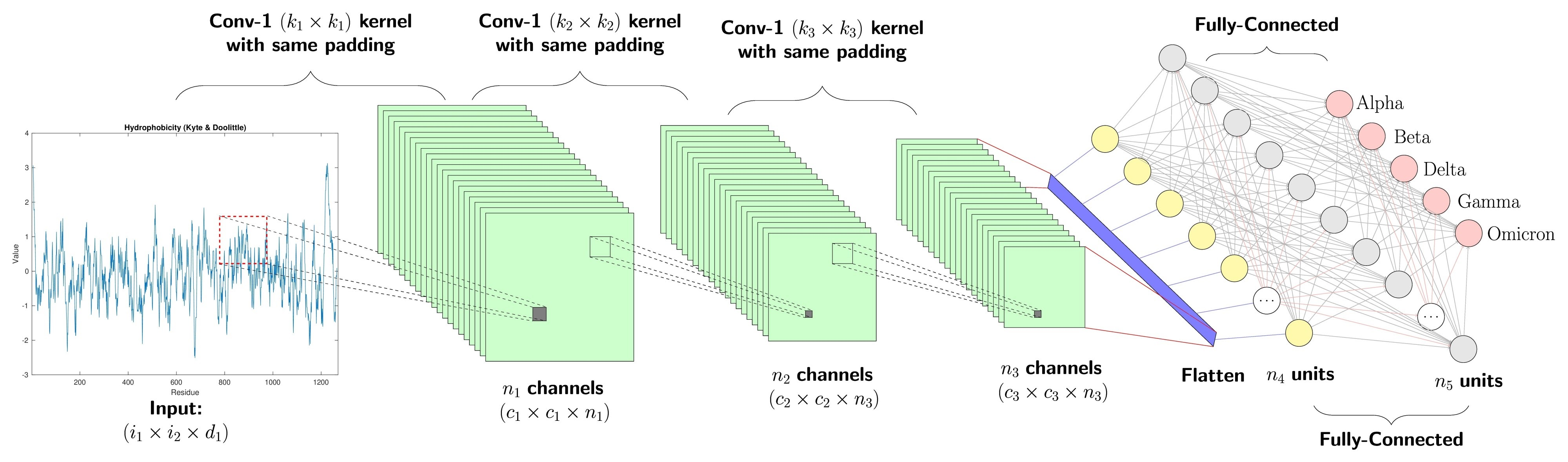
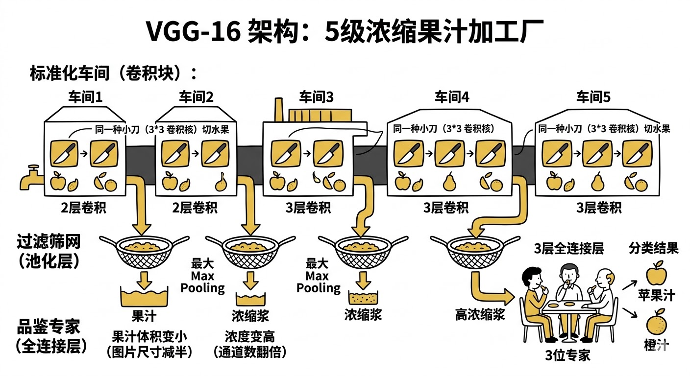
1.1、网络架构与“积木”结构
为了理解 VGG-16 的架构,我们可以把它想象成一个“5级浓缩果汁加工厂”。
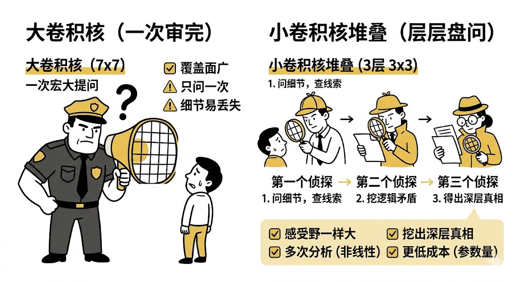
1.2、核心创新:为什么是 3x3?
为了理解为什么要“舍大求小”,我们可以想象 “警察审讯嫌疑人” 的场景。
1.3、从输入到输出的流程
把 VGG-16 想象成一条“数据流水线”。我们将追踪一张猫的照片**(224 * 224 像素)是如何进入网络,被层层“扒皮”,最后变成一个简单的单词“Cat”的。
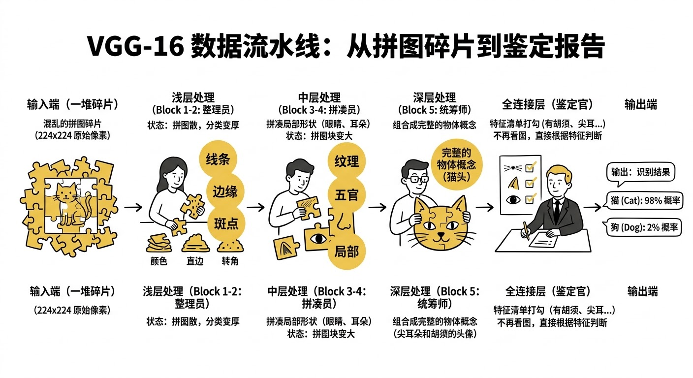
到现在为止,你已经掌握了 VGG-16 的架构 (2-2-3-3-3)、核心原理 (小卷积核) 以及数据流向 (宽变窄,薄变厚)。
二、代码实现
1、准备工作
1.1.设置GPU
import tensorflow as tf
gpus = tf.config.list_physical_devices("GPU")

if gpus:
    gpu0 = gpus[0] #如果有多个GPU,仅使用第0个GPU
    tf.config.experimental.set_memory_growth(gpu0, True) #设置GPU显存用量按需使用
    tf.config.set_visible_devices([gpu0],"GPU")

print(gpus)
2026-04-02 08:55:14.743628: I tensorflow/core/util/util.cc:169] oneDNN custom operations are on. You may see slightly different numerical results due to floating-point round-off errors from different computation orders. To turn them off, set the environment variable `TF_ENABLE_ONEDNN_OPTS=0`.
[PhysicalDevice(name='/physical_device:GPU:0', device_type='GPU')]1.2.导入数据
import os,PIL,pathlib
import matplotlib.pyplot as plt
import numpy             as np
from tensorflow          import keras
from tensorflow.keras    import layers,models

# 查看当前工作路径(确认路径是否正确)
print("当前工作路径:", os.getcwd())

# 定义数据目录(建议用绝对路径更稳妥,相对路径依赖当前工作路径)
data_dir = './data/day09/'
data_dir = pathlib.Path(data_dir)

# 获取数据目录下的所有子路径(文件夹或文件)
data_paths = list(data_dir.glob('*'))

# 提取每个子路径的名称(即类别名,自动适配系统分隔符)
classeNames = [path.name for path in data_paths]
classeNames
当前工作路径: /root/autodl-tmp/TensorFlow2
['cat', 'dog']1.3.查看数据
image_count = len(list(data_dir.glob('*/*')))
print("图片总数为:",image_count)
图片总数为: 34001.4.可视化图片
roses = list(data_dir.glob('dog/*.jpg'))
PIL.Image.open(str(roses[0]))
2、数据预处理
2.1.加载数据
- 使用image_dataset_from_directory方法将磁盘中的数据加载到tf.data.Dataset中
batch_size = 64
img_height = 224
img_width = 224

#训练集
train_ds = tf.keras.preprocessing.image_dataset_from_directory(
    data_dir,
    validation_split=0.2,
    subset="training",
    seed=12,
    image_size=(img_height, img_width),
    batch_size=batch_size)
Found 3400 files belonging to 2 classes.
Using 2720 files for training.
2026-04-02 09:10:01.194533: I tensorflow/core/platform/cpu_feature_guard.cc:193] This TensorFlow binary is optimized with oneAPI Deep Neural Network Library (oneDNN) to use the following CPU instructions in performance-critical operations: AVX2 AVX512F AVX512_VNNI FMA
To enable them in other operations, rebuild TensorFlow with the appropriate compiler flags.
2026-04-02 09:10:02.440253: I tensorflow/core/common_runtime/gpu/gpu_device.cc:1532] Created device /job:localhost/replica:0/task:0/device:GPU:0 with 9960 MB memory: -> device: 0, name: NVIDIA GeForce RTX 3080 Ti, pci bus id: 0000:d9:00.0, compute capability: 8.6# 验证集
val_ds = tf.keras.preprocessing.image_dataset_from_directory(
data_dir,
validation_split=0.2,
subset="validation",
seed=12,
image_size=(img_height, img_width),
batch_size=batch_size)Found 3400 files belonging to 2 classes.
Using 680 files for validation.class_names = train_ds.class_names
print(class_names)['cat', 'dog']2.2.检查数据
- Image_batch是形状的张量(32,180,180,3)。这是一批形状180x180x3的32张图片(最后一维指的是彩色通道RGB)。
- Label_batch是形状(32,)的张量,这些标签对应32张图片
for image_batch, labels_batch in train_ds:
    print(image_batch.shape)
    print(labels_batch.shape)
    break
(64, 224, 224, 3)
(64,)2.3.配置数据集
- shuffle() :打乱数据,关于此函数的详细介绍可以参考
- prefetch() :预取数据,加速运行
- cache() :将数据集缓存到内存当中,加速运行
AUTOTUNE = tf.data.AUTOTUNE

def preprocess_image(image,label):
    return (image/255.0,label)

# 归一化处理
train_ds = train_ds.map(preprocess_image, num_parallel_calls=AUTOTUNE)
val_ds   = val_ds.map(preprocess_image, num_parallel_calls=AUTOTUNE)

train_ds = train_ds.cache().shuffle(1000).prefetch(buffer_size=AUTOTUNE)
val_ds   = val_ds.cache().prefetch(buffer_size=AUTOTUNE)
2.4. 可视化数据
plt.figure(figsize=(15, 10))  # 图形的宽为15高为10

for images, labels in train_ds.take(1):
    for i in range(8):

        ax = plt.subplot(5, 8, i + 1)
        plt.imshow(images[i])
        plt.title(class_names[labels[i]])

        plt.axis("off")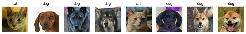
3、训练模型
3.1.构建VGG-16网络
- VGG优点:
VGG的结构非常简洁,整个网络都使用了同样大小的卷积核尺寸(3x3)和最大池化尺寸(2x2)。
- VGG缺点:
-
- 训练时间过长,调参难度大。
-
- 需要的存储容量大,不利于部署。例如存储VGG-16权重值文件的大小为500多MB,不利于安装到嵌入式系统中。
- 结构说明:
-
- 13个卷积层(Convolutional Layer),分别用blockX_convX表示
-
- 3个全连接层(Fully connected Layer),分别用fcX与predictions表示
-
- 5个池化层(Pool layer),分别用blockX_pool表示
- VGG-16包含了16个隐藏层(13个卷积层和3个全连接层),故称为VGG-16
from tensorflow.keras import layers, models, Input
from tensorflow.keras.models import Model
from tensorflow.keras.layers import Conv2D, MaxPooling2D, Dense, Flatten, Dropout

def VGG16(nb_classes, input_shape):
    input_tensor = Input(shape=input_shape)
    # 1st block
    x = Conv2D(64, (3,3), activation='relu', padding='same',name='block1_conv1')(input_tensor)
    x = Conv2D(64, (3,3), activation='relu', padding='same',name='block1_conv2')(x)
    x = MaxPooling2D((2,2), strides=(2,2), name = 'block1_pool')(x)
    # 2nd block
    x = Conv2D(128, (3,3), activation='relu', padding='same',name='block2_conv1')(x)
    x = Conv2D(128, (3,3), activation='relu', padding='same',name='block2_conv2')(x)
    x = MaxPooling2D((2,2), strides=(2,2), name = 'block2_pool')(x)
    # 3rd block
    x = Conv2D(256, (3,3), activation='relu', padding='same',name='block3_conv1')(x)
    x = Conv2D(256, (3,3), activation='relu', padding='same',name='block3_conv2')(x)
    x = Conv2D(256, (3,3), activation='relu', padding='same',name='block3_conv3')(x)
    x = MaxPooling2D((2,2), strides=(2,2), name = 'block3_pool')(x)
    # 4th block
    x = Conv2D(512, (3,3), activation='relu', padding='same',name='block4_conv1')(x)
    x = Conv2D(512, (3,3), activation='relu', padding='same',name='block4_conv2')(x)
    x = Conv2D(512, (3,3), activation='relu', padding='same',name='block4_conv3')(x)
    x = MaxPooling2D((2,2), strides=(2,2), name = 'block4_pool')(x)
    # 5th block
    x = Conv2D(512, (3,3), activation='relu', padding='same',name='block5_conv1')(x)
    x = Conv2D(512, (3,3), activation='relu', padding='same',name='block5_conv2')(x)
    x = Conv2D(512, (3,3), activation='relu', padding='same',name='block5_conv3')(x)
    x = MaxPooling2D((2,2), strides=(2,2), name = 'block5_pool')(x)
    # full connection
    x = Flatten()(x)
    x = Dense(4096, activation='relu',  name='fc1')(x)
    x = Dense(4096, activation='relu', name='fc2')(x)
    output_tensor = Dense(nb_classes, activation='softmax', name='predictions')(x)

    model = Model(input_tensor, output_tensor)
    return model

model=VGG16(1000, (img_width, img_height, 3))
model.summary()
Model: "model"
_________________________________________________________________
Layer (type) Output Shape Param #
=================================================================
input_1 (InputLayer) [(None, 224, 224, 3)] 0
block1_conv1 (Conv2D) (None, 224, 224, 64) 1792
block1_conv2 (Conv2D) (None, 224, 224, 64) 36928
block1_pool (MaxPooling2D) (None, 112, 112, 64) 0
block2_conv1 (Conv2D) (None, 112, 112, 128) 73856
block2_conv2 (Conv2D) (None, 112, 112, 128) 147584
block2_pool (MaxPooling2D) (None, 56, 56, 128) 0
block3_conv1 (Conv2D) (None, 56, 56, 256) 295168
block3_conv2 (Conv2D) (None, 56, 56, 256) 590080
block3_conv3 (Conv2D) (None, 56, 56, 256) 590080
block3_pool (MaxPooling2D) (None, 28, 28, 256) 0
block4_conv1 (Conv2D) (None, 28, 28, 512) 1180160
block4_conv2 (Conv2D) (None, 28, 28, 512) 2359808
block4_conv3 (Conv2D) (None, 28, 28, 512) 2359808
block4_pool (MaxPooling2D) (None, 14, 14, 512) 0
block5_conv1 (Conv2D) (None, 14, 14, 512) 2359808
block5_conv2 (Conv2D) (None, 14, 14, 512) 2359808
block5_conv3 (Conv2D) (None, 14, 14, 512) 2359808
block5_pool (MaxPooling2D) (None, 7, 7, 512) 0
flatten (Flatten) (None, 25088) 0
fc1 (Dense) (None, 4096) 102764544
fc2 (Dense) (None, 4096) 16781312
predictions (Dense) (None, 1000) 4097000
=================================================================
Total params: 138,357,544
Trainable params: 138,357,544
Non-trainable params: 0
_________________________________________________________________3.2.编译模型
在准备对模型进行训练之前,还需要再对其进行一些设置。以下内容是在模型的编译步骤中添加的:
- 损失函数(loss):用于衡量模型在训练期间的准确率。
- 优化器(optimizer):决定模型如何根据其看到的数据和自身的损失函数进行更新。
- 评价函数(metrics):用于监控训练和测试步骤。以下示例使用了准确率,即被正确分类的图像的比率。
model.compile(optimizer="adam",
              loss     ='sparse_categorical_crossentropy',
              metrics  =['accuracy'])
3.3.训练模型
from tqdm import tqdm
import tensorflow.keras.backend as K

epochs = 10
lr     = 1e-4

# 记录训练数据,方便后面的分析
history_train_loss     = []
history_train_accuracy = []
history_val_loss       = []
history_val_accuracy   = []

for epoch in range(epochs):
    train_total = len(train_ds)
    val_total   = len(val_ds)

    """
    total:预期的迭代数目
    ncols:控制进度条宽度
    mininterval:进度更新最小间隔,以秒为单位(默认值:0.1)
    """
    with tqdm(total=train_total, desc=f'Epoch {epoch + 1}/{epochs}',mininterval=1,ncols=100) as pbar:

        lr = lr*0.92
        K.set_value(model.optimizer.lr, lr)

        train_loss     = []
        train_accuracy = []
        for image,label in train_ds:
            """
            训练模型,简单理解train_on_batch就是:它是比model.fit()更高级的一个用法
            """
             # 这里生成的是每一个batch的acc与loss
            history = model.train_on_batch(image,label)

            train_loss.append(history[0])
            train_accuracy.append(history[1])

            pbar.set_postfix({"train_loss": "%.4f"%history[0],
                              "train_acc":"%.4f"%history[1],
                              "lr": K.get_value(model.optimizer.lr)})
            pbar.update(1)

        history_train_loss.append(np.mean(train_loss))
        history_train_accuracy.append(np.mean(train_accuracy))

    print('开始验证!')

    with tqdm(total=val_total, desc=f'Epoch {epoch + 1}/{epochs}',mininterval=0.3,ncols=100) as pbar:

        val_loss     = []
        val_accuracy = []
        for image,label in val_ds:
            # 这里生成的是每一个batch的acc与loss
            history = model.test_on_batch(image,label)

            val_loss.append(history[0])
            val_accuracy.append(history[1])

            pbar.set_postfix({"val_loss": "%.4f"%history[0],
                              "val_acc":"%.4f"%history[1]})
            pbar.update(1)
        history_val_loss.append(np.mean(val_loss))
        history_val_accuracy.append(np.mean(val_accuracy))

    print('结束验证!')
    print("验证loss为:%.4f"%np.mean(val_loss))
    print("验证准确率为:%.4f"%np.mean(val_accuracy))
Epoch 1/10: 0%| | 0/43 [00:00<?, ?it/s]2026-04-02 09:18:40.335169: I tensorflow/stream_executor/cuda/cuda_dnn.cc:384] Loaded cuDNN version 8101
2026-04-02 09:18:47.267058: W tensorflow/core/common_runtime/bfc_allocator.cc:360] Garbage collection: deallocate free memory regions (i.e., allocations) so that we can re-allocate a larger region to avoid OOM due to memory fragmentation. If you see this message frequently, you are running near the threshold of the available device memory and re-allocation may incur great performance overhead. You may try smaller batch sizes to observe the performance impact. Set TF_ENABLE_GPU_GARBAGE_COLLECTION=false if you'd like to disable this feature.
Epoch 1/10: 100%|███| 43/43 [00:22<00:00, 1.90it/s, train_loss=0.7120, train_acc=0.5156, lr=9.2e-5]
开始验证!
Epoch 1/10: 100%|██████████████████| 11/11 [00:02<00:00, 4.19it/s, val_loss=0.7243, val_acc=0.5250]
结束验证!
验证loss为:0.6862
验证准确率为:0.5193
....
Epoch 10/10: 100%|█| 43/43 [00:11<00:00, 3.82it/s, train_loss=0.0604, train_acc=0.9844, lr=4.34e-5]
开始验证!
Epoch 10/10: 100%|█████████████████| 11/11 [00:01<00:00, 9.02it/s, val_loss=0.0716, val_acc=0.9750]
结束验证!
验证loss为:0.0554
验证准确率为:0.97934、模型评估
4.1.Loss与Accuracy图
from datetime import datetime
current_time = datetime.now() # 获取当前时间

epochs_range = range(epochs)

plt.figure(figsize=(14, 4))
plt.subplot(1, 2, 1)

plt.plot(epochs_range, history_train_accuracy, label='Training Accuracy')
plt.plot(epochs_range, history_val_accuracy, label='Validation Accuracy')
plt.legend(loc='lower right')
plt.title('Training and Validation Accuracy')
plt.xlabel(current_time) # 打卡请带上时间戳,否则代码截图无效

plt.subplot(1, 2, 2)
plt.plot(epochs_range, history_train_loss, label='Training Loss')
plt.plot(epochs_range, history_val_loss, label='Validation Loss')
plt.legend(loc='upper right')
plt.title('Training and Validation Loss')
plt.show()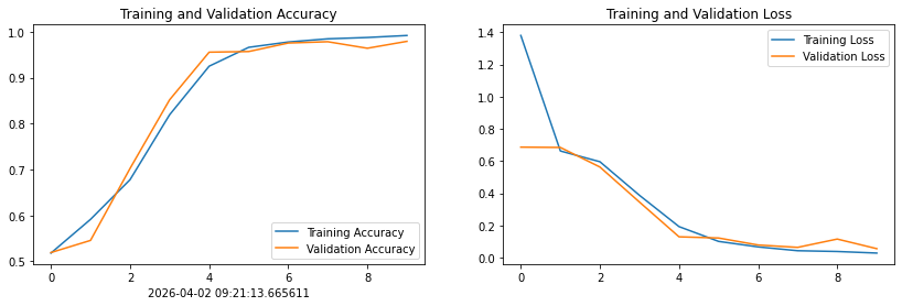
5、图片预测
import numpy as np

# 采用加载的模型(new_model)来看预测结果
plt.figure(figsize=(18, 3))  # 图形的宽为18高为5
plt.suptitle("predict result")

for images, labels in val_ds.take(1):
    for i in range(8):
        ax = plt.subplot(1,8, i + 1)

        # 显示图片
        plt.imshow(images[i].numpy())

        # 需要给图片增加一个维度
        img_array = tf.expand_dims(images[i], 0)

        # 使用模型预测图片中的人物
        predictions = model.predict(img_array)
        plt.title(class_names[np.argmax(predictions)])

        plt.axis("off")
1/1 [==============================] - 0s 29ms/step
1/1 [==============================] - 0s 27ms/step
1/1 [==============================] - 0s 23ms/step
1/1 [==============================] - 0s 26ms/step
1/1 [==============================] - 0s 27ms/step
1/1 [==============================] - 0s 25ms/step
1/1 [==============================] - 0s 25ms/step
1/1 [==============================] - 0s 24ms/step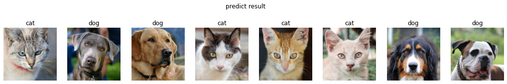

AtomGit 是由开放原子开源基金会联合 CSDN 等生态伙伴共同推出的新一代开源与人工智能协作平台。平台坚持“开放、中立、公益”的理念,把代码托管、模型共享、数据集托管、智能体开发体验和算力服务整合在一起,为开发者提供从开发、训练到部署的一站式体验。
更多推荐


 6
6 0
0- 0


 已为社区贡献8条内容

所有评论(0)