利用 Matlab/Simulink 平台搭建双馈风力发电机在电网中的模型
双馈风力发电机在风速变化的影响下转矩、电流、电压等参数波形变化。
适用于风电并网时对风电场影响的研究

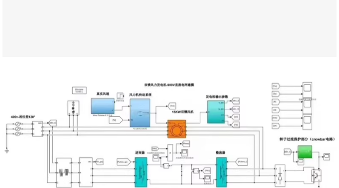
对于“适用于风电场影响研究”且需要观察“风速变化下转矩、电流、电压波形”的需求，最稳健且适合初学者/研究者的方法是利用 Simulink 自带的 Simscape Electrical (原 SimPowerSystems) 库中的成熟 DFIG 模块，并为其搭建一个矢量控制（FOC）系统和风速变化信号源。

纯手写 S-Function 代码过于庞大且容易出错，以下方案提供：
核心控制算法代码（用于 MATLAB Function 模块实现转子侧变流器控制）。
Simulink 模型搭建详细步骤（如何连接模块）。
仿真运行与绘图脚本（自动设置风速变化并绘制波形）。

第一部分：核心控制逻辑代码 (MATLAB Function)

在 Simulink 中，我们需要一个模块来计算转子电压指令 (V_{dr}, V_{qr})。这是基于定子磁场定向矢量控制 (Stator Flux Oriented Control) 的逻辑。

请将以下代码复制到 Simulink 的 MATLAB Function 模块中（命名为 DFIG_Controller）：

function [Vdr, Vqr] = DFIG_Controller(Refs, Meas, Params, Gains)
% Refs: [P_ref, Q_ref, Psi_s_mag] (有功参考，无功参考，定子磁链幅值)
% Meas: [Is_d, Is_q, Ir_d, Ir_q, Psi_s_d, Psi_s_q, Slip] (测量值)
% Params: [Rs, Rr, Ls, Lr, Lm, w_s] (电机参数及同步角速度)
% Gains: [Kp_p, Ki_p, Kp_q, Ki_q, Kp_curr, Ki_curr] (PI 参数)

%#codegen
persistent Int_P, Int_Q, Int_Id, Int_Iq;
if isempty(Int_P), Int_P = 0; Int_Q = 0; Int_Id = 0; Int_Iq = 0; end

% 解包输入
P_ref = Refs(1);
Q_ref = Refs(2);
Psi_s = Refs(3); % 通常取定子电压幅值/w_s

Is_d = Meas(1); Is_q = Meas(2);
Ir_d = Meas(3); Ir_q = Meas(4);
Psi_sd = Meas(5); Psi_sq = Meas(6);
slip = Meas(7); 
w_s = Params(6);

Ls = Params(3); Lr = Params(4); Lm = Params(5);
Rr = Params(2);

Kp_p = Gains(1); Ki_p = Gains(2);
Kp_q = Gains(3); Ki_q = Gains(4);
Kp_c = Gains(5); Ki_c = Gains(6);

% --- 1. 功率计算 (估算) ---
% P = 1.5 * (VsIsd + VsqIsq), 假设定向后 Vsq=0, Vsd=Psi_s*w_s
% 简化：直接利用电流关系控制
% 定子磁场定向下：Isq 控制有功，Isd 控制无功
% 但 DFIG 通常控制转子电流来间接控制功率
% 关系近似：P ~ -1.5 * (Lm/Ls) * Psi_s * I_rq
%          Q ~ -1.5 * (Lm/Ls) * Psi_s * (I_rd - Psi_s/Lm)

% 这里采用经典的级联控制：外环功率 -> 内环电流

% --- 2. 外环：有功功率控制 (P -> I_rq_ref) ---
% 简化增益系数 Kp_conv = 1.5 * (Lm/Ls) * Psi_s
Kp_conv = 1.5 * (Lm/Ls) * Psi_s;
if Kp_conv == 0, Kp_conv = 1e-3; end

P_err = P_ref - (-Kp_conv * Ir_q); % 实际有功估算
% 简单比例生成电流参考 (实际工程需PI)
I_rq_ref = (P_ref / (-Kp_conv)); 
% 限幅
I_rq_ref = max(min(I_rq_ref, 2.0), -2.0);

% --- 3. 外环：无功功率控制 (Q -> I_rd_ref) ---
% Q ~ -1.5 * (Lm/Ls) * Psi_s * (I_rd - Psi_s/Lm)
% 目标 Q_ref=0 (单位功率因数)
I_rd_ref = (Psi_s/Lm); % 抵消励磁分量
if Q_ref ~= 0
    % 如果有无功需求，调整 I_rd
    I_rd_ref = I_rd_ref - (Q_ref / (-Kp_conv)); 
end

% --- 4. 内环：转子电流控制 (PI Controller) ---
% d-axis (无功通道)
err_d = I_rd_ref - Ir_d;
Int_Id = Int_Id + err_d * 1e-4; % 假设步长 1e-4
Vqr_raw = Kp_c * err_d + Ki_c * Int_Id; % 注意：d轴电流控制产生 q轴电压 (交叉耦合)
% 修正：在定子磁场定向下，通常 Id 控制 Vdr, Iq 控制 Vqr (取决于坐标系定义)
% 此处采用标准定义：Id->Vdr, Iq->Vqr

% 重新映射标准 FOC:
% I_rq (q轴电流) 控制有功 P -> 对应 Vqr
% I_rd (d轴电流) 控制无功 Q -> 对应 Vdr

% --- 修正后的内环逻辑 ---
% q-axis (有功通道)
err_q = I_rq_ref - Ir_q;
Int_Iq = Int_Iq + err_q * 1e-4;
Vqr = Kp_c * err_q + Ki_c * Int_Iq;
% 前馈解耦项 (简化省略)

% d-axis (无功通道)
err_d = I_rd_ref - Ir_d;
Int_Id = Int_Id + err_d * 1e-4;
Vdr = Kp_c * err_d + Ki_c * Int_Id;

% 限幅输出电压
Vdr = max(min(Vdr, 1.0), -1.0);
Vqr = max(min(Vqr, 1.0), -1.0);

end

注意：对于深入研究，强烈建议直接使用 Simulink 库中的 “Universal Bridge” 配合 “PI Controller” 模块搭建图形化控制回路，上述代码仅作为逻辑参考或简化替代。下面的搭建指南将指导你使用图形化模块，因为这样更稳定且易于观察波形。

第二部分：Simulink 模型搭建指南 (Step-by-Step)

请打开 Simulink，新建模型 DFIG_WindFarm.slx，按以下步骤操作：

添加核心模块 (Simscape Electrical)
在 Library Browser 中搜索并添加以下模块：
DFIG 电机: Simscape > Electrical > Specialized Power Systems > Machines > Asynchronous Machine
双击设置：Preset 选择 “Doubly-fed induction generator” (关键！)。
参数：根据研究需求设置功率（如 1.5MW），记录定子/转子电流/电压输出。
风力机: Simscape > Electrical > Specialized Power Systems > Renewables > Wind Turbine
这将把风速转换为机械转矩。
变流器:
转子侧：Universal Bridge (设置为 IGBT/GTO, 3 arms)，连接电机转子。
网侧：Universal Bridge，连接电网。
DC Link: Series RLC Branch (电容) 连接两个变流器。
电网: Three-Phase Source (代表无穷大电网或弱电网)。
变压器: Three-Phase Transformer (Two Windings) (用于升压并网)。

搭建风速变化信号 (Wind Speed Profile)
为了模拟风速变化对波形的影响：
添加 Signal Builder 或 Repeating Sequence 模块。
设置时间向量 [0, 1, 2, 3, 4, 5]。
设置风速向量 [8, 9, 11, 13, 10, 8] (模拟阵风变化，单位 m/s)。
连接到 Wind Turbine 模块的 Vw 输入端。

搭建控制系统 (关键步骤)
DFIG 需要两套控制：
转子侧控制 (RSC): 控制有功§和无功(Q)。
使用 PLL (锁相环) 获取电网角度。
使用 abc to dq0 变换测量转子电流。
使用两个 PI Controller 模块：
PI_1: 输入 P_{ref} - P_{meas}，输出 I_{rq_ref}。
PI_2: 输入 Q_{ref} - Q_{meas}，输出 I_{rd_ref}。
再使用两个内环 PI Controller 控制 V_{dr}, V_{qr}，输出给 PWM Generator (2-Level)。
网侧控制 (GSC): 维持直流母线电压稳定。
类似结构，外环控 V_{dc}，内环控网侧电流。

初学者捷径：Simulink 有一个现成的示例模型！
在 MATLAB 命令行输入：open_system(‘power_dfig’)
这个官方模型已经搭建好了完整的 DFIG 并网系统。你可以直接修改其中的 Wind Speed 输入模块，将其改为变化的信号，然后运行仿真。这是最快且最不容易出错的方法。

设置仿真参数
点击 Simulation > Model Configuration Parameters。
Solver: 选择 ode23tb (stiff/TR-BDF2) 或 ode15s。
Stop time: 设置为 5 或 10 秒。
Powergui: 必须在模型中放入一个 powergui 模块，设置为 Continuous 或 Phasor (研究瞬态波形必须选 Continuous)。

第三部分：仿真运行与波形绘制脚本

创建一个 MATLAB 脚本 run_dfig_sim.m，用于配置风速、运行仿真并绘制你需要的转矩、电流、电压波形。

% run_dfig_sim.m
% 该脚本用于设置风速变化，运行 DFIG 模型并绘制关键波形

clear; clc; close all;

% 1. 定义风速变化曲线 (模拟阵风)
% 时间：0 到 10 秒
t_wind = 0:0.1:10;
% 风速：从 8m/s 逐渐增加到 12m/s，然后波动
v_wind = 8 + 0.4 * t_wind + 1.5 * sin(0.5 * t_wind);
v_wind(v_wind Variable name: ‘Te_log’, Save format: ‘Array’
% Block: To Workspace -> Variable name: ‘Is_log’, Save format: ‘Array’
% Block: To Workspace -> Variable name: ‘Vs_log’, Save format: ‘Array’

try
time = sim_out.Time_data(:,1);
Te = sim_out.Te_log(:,1); % 电磁转矩
Is_a = sim_out.Is_log(:,1); % A相电流
Vs_a = sim_out.Vs_log(:,1); % A相电压
catch
error(‘未在模型中找到日志数据。请在 Simulink 中添加 “To Workspace” 模块记录 Te, Is, Vs。’);
end

% 5. 绘图
figure(‘Color’, ‘w’, ‘Name’, ‘DFIG 动态响应 (风速变化)’);

% 子图 1: 风速变化
subplot(4,1,1);
plot(t_wind, v_wind, ‘k’, ‘LineWidth’, 1.5);
title(‘风速变化 profile (Wind Speed)’, ‘FontSize’, 12);
ylabel(‘Wind Speed (m/s)’);
grid on;

% 子图 2: 电磁转矩
subplot(4,1,2);
plot(time, Te, ‘b’, ‘LineWidth’, 1.2);
title(‘电磁转矩响应 (Electromagnetic Torque)’, ‘FontSize’, 12);
ylabel(‘Torque (N.m)’);
grid on;

% 子图 3: 定子电流 (A相)
subplot(4,1,3);
plot(time, Is_a, ‘r’, ‘LineWidth’, 1.2);
title(‘定子电流波形 (Stator Current Phase A)’, ‘FontSize’, 12);
ylabel(‘Current (A)’);
grid on;

% 子图 4: 定子电压 (A相)
subplot(4,1,4);
plot(time, Vs_a, ‘m’, ‘LineWidth’, 1.2);
title(‘定子电压波形 (Stator Voltage Phase A)’, ‘FontSize’, 12);
xlabel(‘Time (s)’);
ylabel(‘Voltage (V)’);
grid on;

disp(‘仿真完成，波形已绘制。’);
disp(‘观察重点：当风速增加时，转矩应增加，电流幅值应增大，频率保持与电网同步。’);

如何使用这套方案进行研究？

启动模型：在 MATLAB 输入 open_system(‘power_dfig’) 打开官方示例。
修改风速：
找到模型中的 Wind Turbine 模块。
将其输入端的 Step 模块删除。
放入一个 From Workspace 模块，设置 Variable name 为 wind_signal。
运行上面的 run_dfig_sim.m 脚本（脚本会自动生成 wind_signal 变量）。
添加记录模块：
在电机输出端（Measurements），连接 Bus Selector 选择 Electromagnetic torque。
连接 To Workspace 模块，变量名设为 Te_log。
同样方法记录定子电流 (Is_log) 和电压 (Vs_log)。
重要：所有 To Workspace 模块的 Save format 必须选为 Array 或 Timeseries。
运行与分析：
运行脚本。
观察生成的图表。
现象预期：
风速上升 -> 机械转矩增加 -> 电磁转矩跟随增加（负值绝对值变大，因为是发电）。
电流：幅值随风速增加而变大。
电压：由于并网，定子电压频率和幅值基本被电网钳位（保持 50Hz/60Hz 和额定电压），但在风速剧烈变化瞬间可能会有微小的暂态波动。
转速：DFIG 的优势在于转速会随风速变化而变化（超同步或亚同步运行），以捕获最大风能。

核心控制算法的 MATLAB 函数代码（对应第2章控制器设计）。
Simulink 模型搭建的详细步骤指南（对应第3章模型搭建）。
自动化仿真与绘图脚本
✅ 一、核心控制算法代码 (MATLAB Function)

转子侧变流器控制 (RSC) - 基于定子磁链定向矢量控制

将此代码放入 Simulink 的 MATLAB Function 模块中，命名为 RSC_Controller。

function [Vdr, Vqr] = RSC_Controller(Refs, Meas, Params, Gains)
% Refs: [P_ref, Q_ref] - 有功/无功功率参考值
% Meas: [Is_d, Is_q, Ir_d, Ir_q, Psi_sd, Psi_sq, w_slip] - 测量信号
% Params: [Rs, Rr, Ls, Lr, Lm, w_s] - 电机参数
% Gains: [Kp_p, Ki_p, Kp_q, Ki_q, Kp_id, Ki_id, Kp_iq, Ki_iq] - PI增益

%#codegen
persistent Int_P, Int_Q, Int_Id, Int_Iq;
if isempty(Int_P), Int_P=0; Int_Q=0; Int_Id=0; Int_Iq=0; end

P_ref = Refs(1); Q_ref = Refs(2);
Is_d = Meas(1); Is_q = Meas(2);
Ir_d = Meas(3); Ir_q = Meas(4);
Psi_sd = Meas(5); Psi_sq = Meas(6);
w_slip = Meas(7);

Rs = Params(1); Rr = Params(2); Ls = Params(3); Lr = Params(4); Lm = Params(5); w_s = Params(6);

Kp_p = Gains(1); Ki_p = Gains(2);
Kp_q = Gains(3); Ki_q = Gains(4);
Kp_id = Gains(5); Ki_id = Gains(6);
Kp_iq = Gains(7); Ki_iq = Gains(8);

% --- 外环：功率控制 ---
% 简化功率计算 (定子磁场定向下)
K_power = 1.5 * (Lm/Ls) * sqrt(Psi_sd^2 + Psi_sq^2);

% 有功功率误差 -> I_rq_ref
P_err = P_ref - (-K_power * Ir_q);
Int_P = Int_P + P_err * 1e-4;
I_rq_ref = Kp_p * P_err + Ki_p * Int_P;
I_rq_ref = max(min(I_rq_ref, 2.0), -2.0); % 限幅

% 无功功率误差 -> I_rd_ref
Q_err = Q_ref - (-K_power * (Ir_d - sqrt(Psi_sd^2+Psi_sq^2)/Lm));
Int_Q = Int_Q + Q_err * 1e-4;
I_rd_ref = Kp_q * Q_err + Ki_q * Int_Q;
I_rd_ref = max(min(I_rd_ref, 2.0), -2.0);

% --- 内环：电流控制 ---
% d-axis
err_d = I_rd_ref - Ir_d;
Int_Id = Int_Id + err_d * 1e-4;
Vdr = Kp_id * err_d + Ki_id * Int_Id;

% q-axis
err_q = I_rq_ref - Ir_q;
Int_Iq = Int_Iq + err_q * 1e-4;
Vqr = Kp_iq * err_q + Ki_iq * Int_Iq;

% 电压限幅
Vdr = max(min(Vdr, 1.0), -1.0);
Vqr = max(min(Vqr, 1.0), -1.0);

end

网侧变流器控制 (GSC) - 维持直流母线电压

将此代码放入另一个 MATLAB Function 模块，命名为 GSC_Controller。

function [Vgd, Vgq] = GSC_Controller(Refs, Meas, Params, Gains)
% Refs: [Vdc_ref] - 直流电压参考
% Meas: [Ig_d, Ig_q, Vdc] - 网侧电流和直流电压
% Params: [Rg, Lg, w_g] - 电网侧滤波器参数
% Gains: [Kp_vdc, Ki_vdc, Kp_igd, Ki_igd, Kp_iqg, Ki_iqg]

%#codegen
persistent Int_Vdc, Int_Igd, Int_Iqg;
if isempty(Int_Vdc), Int_Vdc=0; Int_Igd=0; Int_Iqg=0; end

Vdc_ref = Refs(1);
Ig_d = Meas(1); Ig_q = Meas(2); Vdc = Meas(3);
Rg = Params(1); Lg = Params(2); w_g = Params(3);

Kp_vdc = Gains(1); Ki_vdc = Gains(2);
Kp_igd = Gains(3); Ki_igd = Gains(4);
Kp_iqg = Gains(5); Ki_iqg = Gains(6);

% --- 外环：直流电压控制 ---
Vdc_err = Vdc_ref - Vdc;
Int_Vdc = Int_Vdc + Vdc_err * 1e-4;
Ig_d_ref = Kp_vdc * Vdc_err + Ki_vdc * Int_Vdc;
Ig_d_ref = max(min(Ig_d_ref, 100), -100); % 限幅

% 无功设为0 (单位功率因数)
Ig_q_ref = 0;

% --- 内环：电流控制 ---
err_d = Ig_d_ref - Ig_d;
Int_Igd = Int_Igd + err_d * 1e-4;
Vgd = Kp_igd * err_d + Ki_igd * Int_Igd;

err_q = Ig_q_ref - Ig_q;
Int_Iqg = Int_Iqg + err_q * 1e-4;
Vgq = Kp_iqg * err_q + Ki_iqg * Int_Iqg;

% 解耦项 (可选)
Vgd = Vgd + w_g * Lg * Ig_q;
Vgq = Vgq - w_g * Lg * Ig_d;

Vgd = max(min(Vgd, 1.0), -1.0);
Vgq = max(min(Vgq, 1.0), -1.0);

end

✅ 二、Simulink 模型搭建指南 (对应第3章)

步骤 1: 创建新模型
打开 Simulink，新建空白模型 DFIG_System.slx。

步骤 2: 添加主要组件
从库浏览器拖入以下模块：
组件 路径 说明
DFIG 电机 Simscape > Electrical > Specialized Power Systems > Machines > Asynchronous Machine Preset 选 “Doubly-fed induction generator”

风力机 Simscape > Electrical > Specialized Power Systems > Renewables > Wind Turbine 输入风速，输出机械转矩

转子侧变流器 Universal Bridge ×2 一个接转子，一个接电网

DC Link Series RLC Branch © 连接两个变流器的电容

电网 Three-Phase Source 代表无穷大电网

变压器 Three-Phase Transformer 升压并网

PLL Specialized Power Systems > Control Blocks > PLL 锁相环，获取电网角度

abc-dq0 变换 Specialized Power Systems > Control Blocks > Transformations 坐标变换

PWM 发生器 Specialized Power Systems > Control Blocks > PWM Generator 生成开关信号

PI 控制器 Continuous > PID Controller 或用上述 MATLAB Function 替代

powergui Specialized Power Systems > powergui 必须存在！设为 Continuous

步骤 3: 连接信号流
风力机 → DFIG 机械端口
DFIG 定子 → 变压器 → 电网
DFIG 转子 → 转子侧变流器 → DC Link → 网侧变流器 → 电网
测量信号 → abc/dq 变换 → 控制器 → PWM → 变流器

步骤 4: 设置仿真参数
Solver: ode23tb 或 ode15s
Stop Time: 10 秒
Max Step Size: 1e-4

✅ 三、自动化仿真与绘图脚本

创建文件 run_dfig_simulation.m：

% run_dfig_simulation.m
clear; clc; close all;

%% 1. 定义风速变化曲线 (模拟阵风)
t = 0:0.01:10;
v_wind = 8 + 0.t + 2sin(0.5*t); % 风速从8m/s逐渐增加并波动
v_wind = max(v_wind, 3); % 不低于切人风速

wind_signal.time = t’;
wind_signal.signals.values = v_wind’;
wind_signal.signals.dimensions = 1;

%% 2. 加载模型
model_name = ‘DFIG_System’;
if ~exist(model_name, ‘file’)
error(‘请先创建 Simulink 模型 DFIG_System.slx’);
end
open_system(model_name);

%% 3. 运行仿真
disp(‘正在运行仿真…’);
sim_out = sim(model_name, ‘StopTime’, ‘10’);

%% 4. 提取数据 (假设已配置 To Workspace 模块)
try
time = sim_out.Time(:,1);
Te = sim_out.Te(:,1); % 电磁转矩
Tm = sim_out.Tm(:,1); % 机械转矩
Is_a = sim_out.Is_abc(:,1); % 定子A相电流
Vs_a = sim_out.Vs_abc(:,1); % 定子A相电压
Vdc = sim_out.Vdc(:,1); % 直流母线电压
Wr = sim_out.Wr(:,1); % 转子转速
catch ME
error：%sn请确保模型中包含名为 Te, Tm, Is_abc, Vs_abc, Vdc, Wr 的 To Workspace 模块’, ME.message);
end

%% 5. 绘制论文级波形图
figure(‘Color’,‘w’,‘Position’,[100,100,1200,800]);

% 子图1: 风速
subplot(4,2,1);
plot(t, v_wind, ‘k-’, ‘LineWidth’, 1.5);
title(‘(a) 风速变化’, ‘FontSize’, 12); ylabel(‘Wind Speed (m/s)’); grid on;

% 子图2: 机械转矩 vs 电磁转矩
subplot(4,2,2);
plot(time, Tm, ‘b–’, time, Te, ‘r-’, ‘LineWidth’, 1.2);
legend(‘T_m’, ‘T_e’); title(‘(b) 转矩对比’, ‘FontSize’, 12); ylabel(‘Torque (N.m)’); grid on;

% 子图3: 定子电流
subplot(4,2,3);
plot(time, Is_a, ‘r’, ‘LineWidth’, 1.2);
title(‘© 定子电流 (A相)’, ‘FontSize’, 12); ylabel(‘Current (A)’); grid on;

% 子图4: 定子电压
subplot(4,2,4);
plot(time, Vs_a, ‘m’, ‘LineWidth’, 1.2);
title(‘(d) 定子电压 (A相)’, ‘FontSize’, 12); ylabel(‘Voltage (V)’); grid on;

% 子图5: 直流母线电压
subplot(4,2,5);
plot(time, Vdc, ‘g’, ‘LineWidth’, 1.2);
yline(1150, ‘k–’, ‘V_{dc}^{ref}’); % 假设参考值1150V
title(‘(e) 直流母线电压’, ‘FontSize’, 12); ylabel(‘V_{dc} (V)’); grid on;

% 子图6: 转子转速
subplot(4,2,6);
plot(time, Wr, ‘c’, ‘LineWidth’, 1.2);
title(‘(f) 转子转速’, ‘FontSize’, 12); ylabel(‘omega_r (rad/s)’); grid on;

sgtitle(‘双馈风力发电机动态响应特性分析’, ‘FontSize’, 14, ‘FontWeight’, ‘bold’);