博客笔记逻辑示意图：

1. 关于扩散模型的直觉理解

见《Diffusion 扩散模型知识体系梳理（一）》

2. 从 DDPM 的角度看离散 Diffusion

见《Diffusion 扩散模型知识体系梳理（一）》

3. 从 Score-based 的角度再看 Diffusion

3.1. 如何对目标与环境建模？

• 好的，上来让我们放下先前所有对扩散模型所谓正向加噪/逆向去噪的理解，从另一个角度来审视生成模型这个课题。
• 从本质上讲，我们认为大自然中万物数据 $\mathbf{x}$ 都会存在一种分布关系 $p(\mathbf{x})$，这是我们无法进行精确量化的，所以生成模型则会基于我们能够获取到的数据集 { x 1 , x 2 , ⋯   , x n } \{\mathbf{x}_1,\mathbf{x}_2,\cdots,\mathbf{x}_n\} {x1​,x2​,⋯,xn​}，去尝试用网络拟合这样的分布 $p_{\theta }(\mathbf{x})$。然后，我们知道任何一种概率分布都需要满足归一性与非负性，所以在此处，我们可以为 $p_{\theta }(\mathbf{x})$ 构建一种模型的形态 $$p_{\theta }(\mathbf{x})=\frac{e^{-f_{\theta }(\mathbf{x})}}{Z_{\theta }},\text{where}\int p_{\theta }(\text{x})d\text{x}=1,Z_{\theta }=\int e^{-f_{\theta }(\text{x})}d\text{x}$$ 此处的 $f_{\theta }$ 可以称之为非归一化概率模型，或者能量模型（Energy-Based Model）。

3.2. 如何确定网络学习的目标 ？

• 所以此时我们会关注到，如果我们希望 $p_{\theta }$ 尽可能准确，可以通过最大化似然的方式来描述，同时出于指数幂次连乘变连加的考虑，加上对数作为目标方向（Maximize the log-likelihood）：$$\underset{\theta }{\max }\sum _{i=1}^N\log p_{\theta }(x_i)$$
• 然而，上面的式子要求 $p_{\theta }(\mathbf{x})$ 是一个经过归一化的概率密度函数。这是我们不希望看到的，因为为了计算 $p_{\theta }(\mathbf{x})$，我们必须求出归一化常数 $Z_{\theta }$ ，但是对于任何一般的函数 $f_{\theta }(\mathbf{x})$ 来说，这通常是一个难以计算的量（前人只能通过 VAE 自回归或者 MCMC 采样近似估计等方式处理）。所以我们进行下面的这种定义，可以巧妙地用对数的性质消去常数 $Z_{\theta }$，这就是 Hyvärinen [4] 提出的 Score Matching 的核心思想：$${\mathbf{s}}_{\theta }(\mathbf{x})={\nabla }_{\mathbf{x}}\log p_{\theta }(\mathbf{x})=-{\nabla }_{\mathbf{x}}{f}_{\theta }(\mathbf{x})-\underset{=0}{\underbrace{{\nabla }_{\mathbf{x}}\log Z_{\theta }}}=-{\nabla }_{\mathbf{x}}{f}_{\theta }(\mathbf{x})$$

3.3. 如何构建损失函数 ？

• 很好，那在知道了模型拟合的目标之后，就该要去定义相应的损失函数了。由上文可知，我们为了避开无法计算的 $Z_{\theta }$，采用 Fisher Divergence 作为模型预测的 Loss Function：$$\mathcal{J}(\theta )={\mathbb{E}}_{p_{\text{data}}(\text{x})}[\frac{1}{2}||s_{\theta }(\text{x})-{\nabla }_{\text{x}}\log p_{\text{data}}(\text{x}))|{|}_2^2]$$
• 可是问题是，此时我们还是无法知道我们需要的真实数据分布，但是经过一段巧妙地数学推导（见 Appendix A）上述损失函数可以转化为等价的显式得分匹配 (Explicit Score Matching) 目标：$$\mathcal{J}(\theta )={\mathbb{E}}_{p_{\text{data}}(\text{x})}[\frac{1}{2}||s_{\theta }(\text{x})|{|}^2+\text{tr}({\nabla }_{\text{x}}{s}_{\theta }(\text{x}))]$$
• 这一绝妙的转化使得损失函数不再依赖于真实数据分布的解析形式。在理论上，我们可以直接通过在训练集上采样 $\text{x}$ 来近似该期望。但是，由于计算高维雅可比矩阵的迹 $\text{tr}({\nabla }_{\text{x}}{s}_{\theta }(\text{x}))$ 存在难以承受的计算开销，该方法很难直接应用于高维数据（如图像）。实际工程上，通常有两种解决办法，分别是 Pascal Vincent [5] 提出的 Denoising Score Matching (DSM, 去噪得分匹配，严格推导见 Appendix B)，另一条是 Yang Song et al. [6] 提出的 Sliced Score Matching (SSM, 切片得分匹配，其核心思想是用随机投影向量将高维散度降为一维方向导数，从而避免计算完整的雅可比矩阵，此处不展开)。

3.4. 如何进行采样推理？

• 假设我的模型已经训练好了，分析一下，我们本质上获得的是一个向量场，时刻告诉我们概率密度增加最快的方向是哪里，你可以把它想象成高维势能面上的重力线，它永远指向“更像真实数据”的高密度区域。当我们一直沿着 ${\nabla }_{\text{x}}\log p(\text{x})$ 的方向移动时，最终会确定性地停留在某一个概率密度的峰值（mode），但是这往往并非想要寻找的真实数据分布，所以我们需要在每一步的过程中都添加一项布朗运动。而这个靠近的过程迭代，是基于朗之万动力学（Langevin Dynamics） 所构造的，公式如下：$$x_{i+1}\leftarrow x_i+\frac{ϵ}{2}\cdot {\nabla }_{\text{x}}\log p(\text{x})+\sqrt{ϵ}\cdot z_i,\text{where}i=1\sim k,z_i\sim \mathcal{N}(0,I)$$
• 当然，理想很丰满，现实很骨感，实验发现，如果拿着上面的公式去生成，大概率会得到一堆充满噪点的无意义色块，原因在于真实的物理世界数据（比如人脸图片）在高维空间中满足流形假设 (Manifold Hypothesis)。真实数据只占据高维空间中极其狭窄、低维的流形“薄膜”，而薄膜之外的广袤空间里，真实数据的概率 $p(\text{x})\approx 0$。这会导致两个问题：
  1. 梯度消失或未定义：在纯噪声区域，网络根本没见过这些数据，${\text{s}}_{\theta }(\text{x})$ 的预测是完全瞎猜的，或者梯度为 0。
  2. 孤岛效应： 即使网络预测准了，不同模式（比如“猫”的流形和“狗”的流形）之间是被概率为 0 的大块区域隔开的。朗之万动力学的噪声无法跨越这片区域，导致采样极易卡死在一个局部流形里出不来。

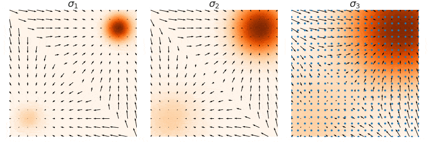
3.5. 如何解决流形分布的问题？

• 研究者们 [7] 提出的方案，是利用噪声对数据点进行扰动，并在这些带噪的数据点上训练基于分数的模型。当噪声的幅度足够大时，它能够填充数据低密度的区域，从而提高估计得分的准确性。至于噪声的分布方差，由于数据集的差异性过大，所以选取从小到大的一组方差序列 { σ 1 , σ 2 , ⋯   , σ L } \{\sigma_1,\sigma_2,\cdots,\sigma_L\} {σ1​,σ2​,⋯,σL​}，通过与原始数据分布进行卷积：$$p_{{\sigma }_i}(\mathbf{x})=\int p(\mathbf{y})\mathcal{N}(\mathbf{x};\mathbf{y},{\sigma }_i^2\mathbf{I})d\mathbf{y}$$ 其中 $\mathcal{N}(\mathbf{x};\mathbf{y},{\sigma }_i^2\mathbf{I})$ 是一个以 $\mathbf{y}$ 为均值、${\sigma }_i^2$ 为方差的高斯分布核。它代表了加在数据上的噪声。至于卷积操作，在代码中只需要从训练集中抽取一个样本 $\text{y}$，再加上相应强度的噪声即可 $\text{y}+{\sigma }_i\text{z}\sim p_{{\sigma }_i}(\text{x})$。
• 自然我们也需要重构一下前面设定的模型训练目标和训练损失函数。我们定义了噪声条件评分模型 Noise Conditional Score-Based Model，也即 $s_{\theta }(\text{x},i)$。而损失函数同样沿用 Fisher Divergence 的思路，公式定义如下：$$\mathcal{J}(\theta )=\sum _{i=1}^N\lambda (i){\mathbb{E}}_{p_{{\sigma }_i}(\text{x})}[\frac{1}{2}||s_{\theta }(\text{x},i)-{\nabla }_{\text{x}}\log p_{{\sigma }_i}(\text{x}))|{|}_2^2]$$ 其中加权系数 $\lambda (i)\propto {\sigma }_i^2$，这么做的目的是为了平衡不同噪声尺度下的损失函数，可以从下面这个维度来理解。假设添加噪声之后的 $\text{x}$ 是满足高斯分布的，那么有：$$p(\mathbf{x}|\mathbf{y})=\mathcal{N}(\mathbf{x};\mathbf{y},{\sigma }_i^2\mathbf{I})=\frac{1}{(2\pi {\sigma }_i^2{)}^{d/2}}\exp \left(-\frac{\Vert \mathbf{x}-\mathbf{y}{\Vert }_2^2}{2{\sigma }_i^2}\right)$$ 取对数后：$$\log p(\mathbf{x}|\mathbf{y})=\underset{\text{常数 }C}{\underbrace{-\frac{d}{2}\log (2\pi {\sigma }_i^2)}}-\frac{\Vert \mathbf{x}-\mathbf{y}{\Vert }_2^2}{2{\sigma }_i^2}$$ 利用链式法则，注意到 ${\nabla }_{\mathbf{x}}\Vert \mathbf{x}-\mathbf{y}{\Vert }_2^2=2(\mathbf{x}-\mathbf{y})$：$$\begin{array}{rl}{\nabla }_{\mathbf{x}}\log p(\mathbf{x}|\mathbf{y})& =0-\frac{1}{2{\sigma }_i^2}\cdot {\nabla }_{\mathbf{x}}(\mathbf{x}-\mathbf{y}{)}^T(\mathbf{x}-\mathbf{y})\\ & =-\frac{1}{2{\sigma }_i^2}\cdot 2(\mathbf{x}-\mathbf{y})=-\frac{\mathbf{x}-\mathbf{y}}{{\sigma }_i^2}\end{array}$$ 因为我们知道 $\mathbf{x}=\mathbf{y}+{\sigma }_i\mathbf{z}$（其中 $\mathbf{z}\sim \mathcal{N}(0,\mathbf{I})$），代入上式即可知道条件 score 的 L2 范数期望 $\mathbb{E}[\Vert {\nabla }_{\mathbf{x}}\log p(\mathbf{x}|\mathbf{y}){\Vert }^2]=\frac{d}{{\sigma }_i^2}$（$d$ 为数据维度），所以 $\lambda (i)\propto {\sigma }_i^2$ 的选取恰好能抵消这个量级差异，使得不同噪声尺度下的损失贡献大致均衡：$${\nabla }_{\mathbf{x}}\log p(\mathbf{x}|\mathbf{y})=-\frac{(\mathbf{y}+{\sigma }_i\mathbf{z})-\mathbf{y}}{{\sigma }_i^2}=-\frac{{\sigma }_i\mathbf{z}}{{\sigma }_i^2}=-\frac{\mathbf{z}}{{\sigma }_i}$$ 但是这里面需要注意的一点是，我们之所以可以用条件分布来估计边缘分布，主要是因为在期望意义上，优化 “模型与条件分布评分的距离”等价于优化“模型与边缘分布评分的距离” ，数学表达式如下：$${\mathbb{E}}_{p_{{\sigma }_i}(\mathbf{x},\mathbf{y})}\left[\Vert {\mathbf{s}}_{\theta }(\mathbf{x},i)-{\nabla }_{\mathbf{x}}\log p(\mathbf{x}|\mathbf{y}){\Vert }_2^2\right]={\mathbb{E}}_{p_{{\sigma }_i}(\mathbf{x})}\left[\Vert {\mathbf{s}}_{\theta }(\mathbf{x},i)-{\nabla }_{\mathbf{x}}\log p_{{\sigma }_i}(\mathbf{x}){\Vert }_2^2\right]+C$$

3.6. 退火朗之万动力学采样

• 针对于前文构造的噪声条件评分模型，我们也应该相应的为之调整一下采样的模式，称之为退火朗之万动力学采样 Annealed Langevin Dynamics。在此所谓的退火，就表示模型会先在较大层面的噪声中确定宏观的轮廓和区域，随后随着噪声的波动越来越小，逐渐锁定迭代到最优的位置。
  1. 第一步，先从纯噪声中随机初始化一个起始点 ${\mathbf{x}}_L^0\sim \mathcal{N}(0,{\sigma }_L^2\mathbf{I})$，此时的 $\mathbf{x}$ 看起来就是完全的随机白噪声。
  2. 第二步，我们考虑从大噪声到小噪声，$i=L,L-1,\dots ,1$，利用当前噪声尺度计算采样的步长 ${\alpha }_i=ϵ\cdot {\sigma }_i^2/{\sigma }_L^2$。
  3. 第三步，对于时间步 $t=1,2,...,T$ 运行下面迭代公式：$${\mathbf{x}}_t={\mathbf{x}}_{t-1}+\frac{{\alpha }_i}{2}{\mathbf{s}}_{\theta }({\mathbf{x}}_{t-1},i)+\sqrt{{\alpha }_i}{\mathbf{z}}_t$$

---

Appendix

Appendix A：Score Matching 到显式目标的严格推导

• 下面我们的目标是证明：$${\mathcal{J}}_{\text{Fisher}}(\theta )={\mathbb{E}}_{p(\mathbf{x})}\left[\frac{1}{2}\Vert s_{\theta }(\mathbf{x})-{\nabla }_{\mathbf{x}}\log p(\mathbf{x}){\Vert }^2\right]⟺{\mathcal{J}}_{\text{ESM}}(\theta )={\mathbb{E}}_{p(\mathbf{x})}\left[\frac{1}{2}\Vert s_{\theta }(\mathbf{x}){\Vert }^2+\nabla \cdot s_{\theta }(\mathbf{x})\right]$$二者只差与 $\theta$ 无关的常数项。为避免符号冗余，以下记 $p(\mathbf{x})\equiv p_{\text{data}}(\mathbf{x})$，${\mathbf{s}}_{\theta }(\mathbf{x})\equiv s_{\theta }(\mathbf{x})$。

• 首先展开平方项：$${\mathcal{J}}_{\text{Fisher}}(\theta )={\mathbb{E}}_p\left[\frac{1}{2}\Vert {\mathbf{s}}_{\theta }{\Vert }^2-{\mathbf{s}}_{\theta }^{\top }\nabla \log p+\frac{1}{2}\Vert \nabla \log p{\Vert }^2\right].$$ 其中最后一项$$C_p\triangleq \frac{1}{2}{\mathbb{E}}_p\Vert \nabla \log p{\Vert }^2$$与模型参数 $\theta$ 无关，可视作常数。关键在交叉项：$$I(\theta )={\mathbb{E}}_p\left[{\mathbf{s}}_{\theta }^{\top }\nabla \log p\right]=\int {\mathbf{s}}_{\theta }(\mathbf{x}{)}^{\top }\nabla p(\mathbf{x})d\mathbf{x}.$$

• 利用散度恒等式我们可以得到：$$\nabla \cdot \left(p{\mathbf{s}}_{\theta }\right)={\mathbf{s}}_{\theta }^{\top }\nabla p+p\nabla \cdot {\mathbf{s}}_{\theta }⟹{\mathbf{s}}_{\theta }^{\top }\nabla p=\nabla \cdot \left(p{\mathbf{s}}_{\theta }\right)-p\nabla \cdot {\mathbf{s}}_{\theta }.$$代回积分得：$$I(\theta )=\int \nabla \cdot \left(p{\mathbf{s}}_{\theta }\right)d\mathbf{x}-\int p\nabla \cdot {\mathbf{s}}_{\theta }d\mathbf{x}.$$若满足常见边界条件（如 $p(\mathbf{x}){\mathbf{s}}_{\theta }(\mathbf{x})$ 在无穷远处衰减足够快），由散度定理有$$\int \nabla \cdot \left(p{\mathbf{s}}_{\theta }\right)d\mathbf{x}=0,$$因此$$I(\theta )=-{\mathbb{E}}_p\left[\nabla \cdot {\mathbf{s}}_{\theta }(\mathbf{x})\right].$$ 所以我们最终得到：$${\mathcal{J}}_{\text{Fisher}}(\theta )={\mathbb{E}}_p\left[\frac{1}{2}\Vert {\mathbf{s}}_{\theta }{\Vert }^2+\nabla \cdot {\mathbf{s}}_{\theta }\right]+C_p.$$忽略常数 $C_p$ 即得显式得分匹配目标：$$\boxed{{\mathcal{J}}_{\text{ESM}}(\theta )={\mathbb{E}}_p\left[\frac{1}{2}\Vert {\mathbf{s}}_{\theta }(\mathbf{x}){\Vert }^2+\mathrm{tr}({\nabla }_{\mathbf{x}}{\mathbf{s}}_{\theta }(\mathbf{x}))\right]}.$$解释：该式不再显式依赖未知的 $\nabla \log p$，但代价是需要计算散度（Jacobian 迹），这正是高维场景下 ESM 难以直接工程化的根源。

Appendix B：DSM 等价性与 DDPM 的噪声预测目标

• 记加噪核$$q_{\sigma }(\tilde{\mathbf{x}}\mid \mathbf{x})=\mathcal{N}(\tilde{\mathbf{x}};\mathbf{x},{\sigma }^2\mathbf{I}),q_{\sigma }(\tilde{\mathbf{x}})=\int q_{\sigma }(\tilde{\mathbf{x}}\mid \mathbf{x})p(\mathbf{x})d\mathbf{x}.$$ DSM 目标是$${\mathcal{J}}_{\text{DSM}}(\theta )={\mathbb{E}}_{p(\mathbf{x})q_{\sigma }(\tilde{\mathbf{x}}\mid \mathbf{x})}\left[\frac{1}{2}{\Vert s_{\theta }(\tilde{\mathbf{x}})-{\nabla }_{\tilde{\mathbf{x}}}\log q_{\sigma }(\tilde{\mathbf{x}}\mid \mathbf{x})\Vert }^2\right].$$

• 假设$$\mathbf{u}(\tilde{\mathbf{x}},\mathbf{x})\triangleq {\nabla }_{\tilde{\mathbf{x}}}\log q_{\sigma }(\tilde{\mathbf{x}}\mid \mathbf{x}),\bar{\mathbf{u}}(\tilde{\mathbf{x}})\triangleq \mathbb{E}[\mathbf{u}(\tilde{\mathbf{x}},\mathbf{x})\mid \tilde{\mathbf{x}}].$$对平方项做条件方差分解：$$\mathbb{E}\Vert s_{\theta }-\mathbf{u}{\Vert }^2=\mathbb{E}\Vert s_{\theta }-\bar{\mathbf{u}}{\Vert }^2+\mathbb{E}\Vert \mathbf{u}-\bar{\mathbf{u}}{\Vert }^2.$$ 第二项与 $\theta$ 无关，因此最优解由第一项决定。所以此时只需证明$$\bar{\mathbf{u}}(\tilde{\mathbf{x}})={\nabla }_{\tilde{\mathbf{x}}}\log q_{\sigma }(\tilde{\mathbf{x}}).$$ 由 Bayes 与求导交换可得下式，两边除以 $q_{\sigma }(\tilde{\mathbf{x}})$ 即得结论。：$${\nabla }_{\tilde{\mathbf{x}}}{q}_{\sigma }(\tilde{\mathbf{x}})=\int {\nabla }_{\tilde{\mathbf{x}}}{q}_{\sigma }(\tilde{\mathbf{x}}\mid \mathbf{x})p(\mathbf{x})d\mathbf{x}=\int q_{\sigma }(\tilde{\mathbf{x}}\mid \mathbf{x})\mathbf{u}(\tilde{\mathbf{x}},\mathbf{x})p(\mathbf{x})d\mathbf{x},$$

• 所以 DSM 实际优化的是
  $${\mathbb{E}}_{q_{\sigma }(\tilde{\mathbf{x}})}\left[\frac{1}{2}\Vert s_{\theta }(\tilde{\mathbf{x}})-\nabla \log q_{\sigma }(\tilde{\mathbf{x}}){\Vert }^2\right]+\text{const}.$$

• 对高斯核有解析 target：$${\nabla }_{\tilde{\mathbf{x}}}\log q_{\sigma }(\tilde{\mathbf{x}}\mid \mathbf{x})=-\frac{\tilde{\mathbf{x}}-\mathbf{x}}{{\sigma }^2}.$$令 $\tilde{\mathbf{x}}=\mathbf{x}+\sigma \mathbf{z}$（$\mathbf{z}\sim \mathcal{N}(0,\mathbf{I})$），则$${\mathcal{J}}_{\text{DSM}}(\theta )={\mathbb{E}}_{p(\mathbf{x}),\mathbf{z}}\left[\frac{1}{2}{\Vert s_{\theta }(\mathbf{x}+\sigma \mathbf{z})+\frac{\mathbf{z}}{\sigma }\Vert }^2\right].$$

• DDPM 的 $ϵ$-prediction 与之对应关系：$${\mathbf{x}}_t=\sqrt{{\bar{\alpha }}_t}{\mathbf{x}}_0+\sqrt{1-{\bar{\alpha }}_t}\mathbf{ϵ}\Rightarrow {\nabla }_{{\mathbf{x}}_t}\log q({\mathbf{x}}_t\mid {\mathbf{x}}_0)=-\frac{\mathbf{ϵ}}{\sqrt{1-{\bar{\alpha }}_t}}.$$因此常见参数化$$s_{\theta }({\mathbf{x}}_t,t)=-\frac{{ϵ}_{\theta }({\mathbf{x}}_t,t)}{\sqrt{1-{\bar{\alpha }}_t}}$$正是 DSM 形式在离散时间上的实现。

---

Reference

[4] Hyvärinen, A. (2005). Estimation of Non-Normalized Statistical Models by Score Matching. JMLR, 6, 695–709.

[5] Vincent, P. (2011). A Connection Between Score Matching and Denoising Autoencoders. Neural Computation, 23(7), 1661–1674.

[6] Song, Y., Garg, S., Shi, J., & Ermon, S. (2020). Sliced Score Matching: A Scalable Approach to Density and Score Estimation. UAI 2020.

[7] Song, Y., & Ermon, S. (2019). Generative Modeling by Estimating Gradients of the Data Distribution. NeurIPS 2019.