🏆 本文收录于专栏 《YOLOv11实战：从入门到深度优化》。
本专栏围绕 YOLOv11 的改进、训练、部署与工程优化 展开，系统梳理并复现当前主流的 YOLOv11 实战案例与优化方案，内容目前已覆盖 分类、检测、分割、追踪、关键点、OBB 检测 等多个方向。

与常见“只给代码、不讲原理”的教程不同，这个专栏更关注 模型为什么这样改、训练为什么这样配、部署为什么这样做，以及出问题后应该如何定位与修正。
如果你希望自己不仅能把项目跑起来，还能进一步具备 调参、优化、迁移和工程落地 的能力，那么这套内容会更适合作为系统学习 YOLOv11 的参考。

专栏整体坚持 持续更新 + 深度解析 + 工程导向 的写作思路，不仅关注模型结构本身，也关注训练策略、损失函数设计、推理加速、部署适配以及真实项目中的问题排查。

✨ 当前专栏限时优惠中：一次订阅，终身有效，后续更新内容均可免费解锁 👉 点此查看专栏详情

🎯 本文定位：计算机视觉 × YOLOv11 零基础入门实战
📅 预计阅读时间：60～90分钟
⭐ 难度等级：⭐⭐☆☆☆（基础级）
🔧 技术栈：Ultralytics YOLO11 | Python v3.9+ | PyTorch v2.0+ | torchvision v0.9+ | Ultralytics v8.x | CUDA v11.8+

📖 上期回顾｜模型推理与性能测试全流程

在上一节《YOLOv11【第一章：零基础入门篇·第4节】一文搞懂，模型推理与性能测试全流程！》内容中，我们深入探讨了 YOLOv11 模型推理与性能测试的完整流程。主要涵盖以下核心内容：

• 推理环境配置：讲解了如何在 CPU / GPU 环境下配置推理运行时，包括 CUDA 版本匹配、PyTorch 推理模式（torch.no_grad()）的使用技巧。
• 图像预处理流程：详细介绍了图像归一化、Letterbox 缩放填充策略、颜色通道转换（BGR→RGB）及 Tensor 维度变换等标准化预处理步骤。
• 推理接口调用：从 Python API 调用、CLI 命令行批量推理、视频流实时推理三个维度系统演示了 YOLOv11 的多种调用方式。
• 后处理解析：深入剖析了 NMS（非极大值抑制）的原理与参数调优，以及检测框坐标解码（xywh → xyxy）的完整逻辑。
• 性能基准测试：使用 time、torch.cuda.Event 等工具对推理速度进行精准计时，并通过 FPS 指标对比不同硬件、不同模型规格（n/s/m/l/x）的性能差异。

💡 核心收获：读者掌握了从原始图像输入到最终检测结果输出的完整推理管线，并能独立完成推理性能基准测试。这为本节的模型验证与量化评估奠定了工程基础。

一、为什么需要模型验证与评估？

在深度学习项目中，训练一个模型只是起点，如何客观、全面地衡量模型的好坏才是决定项目成败的关键环节。很多初学者在训练完模型后，仅凭肉眼观察推理结果就下结论，这种主观判断往往存在严重的偏差。

想象一个场景：你训练了一个行人检测模型，在几张测试图像上看起来效果不错，但实际部署后误检率极高。这就是因为缺乏系统的量化评估——没有数字就没有方向。

1.1 评估的三大核心价值

① 量化模型能力边界

通过 mAP、Precision、Recall 等指标，我们能精确知道模型在哪些类别上表现好、哪些类别存在瓶颈，而不是凭直觉判断。

② 指导模型迭代优化

评估结果是模型改进的"罗盘"：如果 Recall 低，说明模型漏检严重，需要降低置信度阈值或增加正样本数量；如果 Precision 低，说明误检多，需要提高阈值或加强负样本训练。

③ 横向对比与选型

在多个候选模型（如 YOLOv11n vs YOLOv11s vs YOLOv11m）之间进行公平比较，必须有统一的评估标准和测试集，才能做出客观的模型选型决策。

1.2 验证集 vs 测试集

这是一个常见的概念混淆点，必须厘清：

训练集 (Train Set)     → 用于反向传播、更新模型参数
验证集 (Val Set)       → 训练过程中监控泛化性能、调整超参数（有数据泄露风险）
测试集 (Test Set)      → 训练完成后最终评估，模拟真实部署场景（完全隔离）

在 YOLOv11 的标准工作流中，val 命令默认使用验证集进行评估，但最终发论文或汇报时应使用独立测试集。

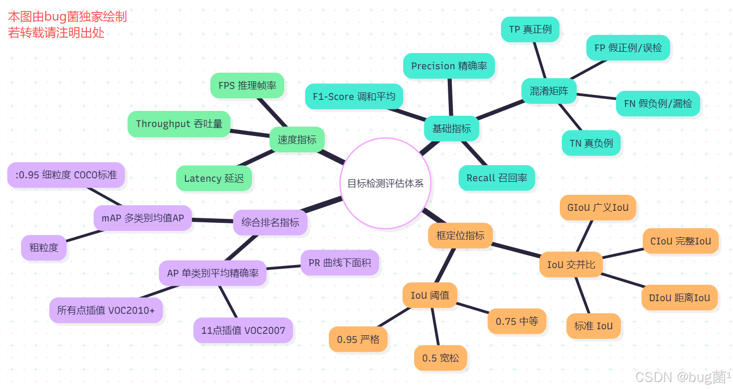
二、目标检测评估指标体系全解

目标检测的评估比图像分类复杂得多，因为它同时涉及定位精度和分类精度两个维度。下面我们从最基础的概念逐步构建完整的评估体系。

2.1 混淆矩阵与基础指标

混淆矩阵（Confusion Matrix）是所有分类与检测任务评估的基石。对于二分类问题（以"是否检测到目标"为例），混淆矩阵定义如下：

                        预测为正 (Positive)    预测为负 (Negative)
真实为正 (Positive)         TP（真正例）           FN（假负例/漏检）
真实为负 (Negative)         FP（假正例/误检）        TN（真负例）

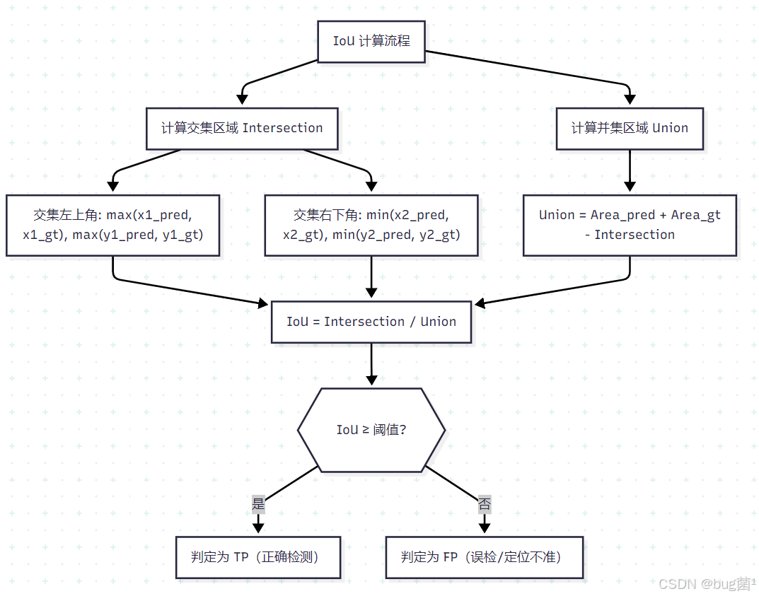
在目标检测中，判定一个预测框是 TP 还是 FP，不仅要看类别是否正确，还要看定位是否准确（通过 IoU 阈值判定）。

基础指标定义：

指标	公式	含义
Precision（精确率）	TP / (TP + FP)	预测为正的样本中真正为正的比例（衡量误检）
Recall（召回率）	TP / (TP + FN)	真实为正的样本中被检测到的比例（衡量漏检）
F1-Score	2×P×R / (P+R)	Precision 与 Recall 的调和平均
Accuracy（准确率）	(TP+TN) / All	整体正确率（目标检测中几乎不用）

⚠️ 注意：在目标检测领域，Accuracy 几乎没有参考价值，因为背景区域（负样本）数量远多于目标区域（正样本），会导致 Accuracy 虚高。

2.2 IoU：检测框质量的核心度量

IoU（Intersection over Union，交并比） 是目标检测中衡量预测框与真实框重叠程度的核心指标，也是判定 TP/FP 的基准。

$$\text{IoU}=\frac{\text{预测框}\cap \text{真实框的面积}}{\text{预测框}\cup \text{真实框的面积}}$$

IoU 阈值的直觉理解：

• IoU = 1.0：预测框与真实框完全重合（理想情况）
• IoU = 0.5：两框重叠面积占并集面积的 50%（PASCAL VOC 标准阈值）
• IoU = 0.75：更严格的定位要求（COCO 标准之一）
• IoU = 0.0：两框完全不重叠

IoU 的变体（进阶了解）：

变体	特点	适用场景
GIoU	引入最小外接矩形，解决不重叠时梯度消失	训练损失函数
DIoU	加入中心点距离惩罚	训练损失函数
CIoU	同时考虑重叠、中心距离、长宽比	YOLOv5/v8/v11 默认损失
SIoU	引入角度信息	部分改进版 YOLO

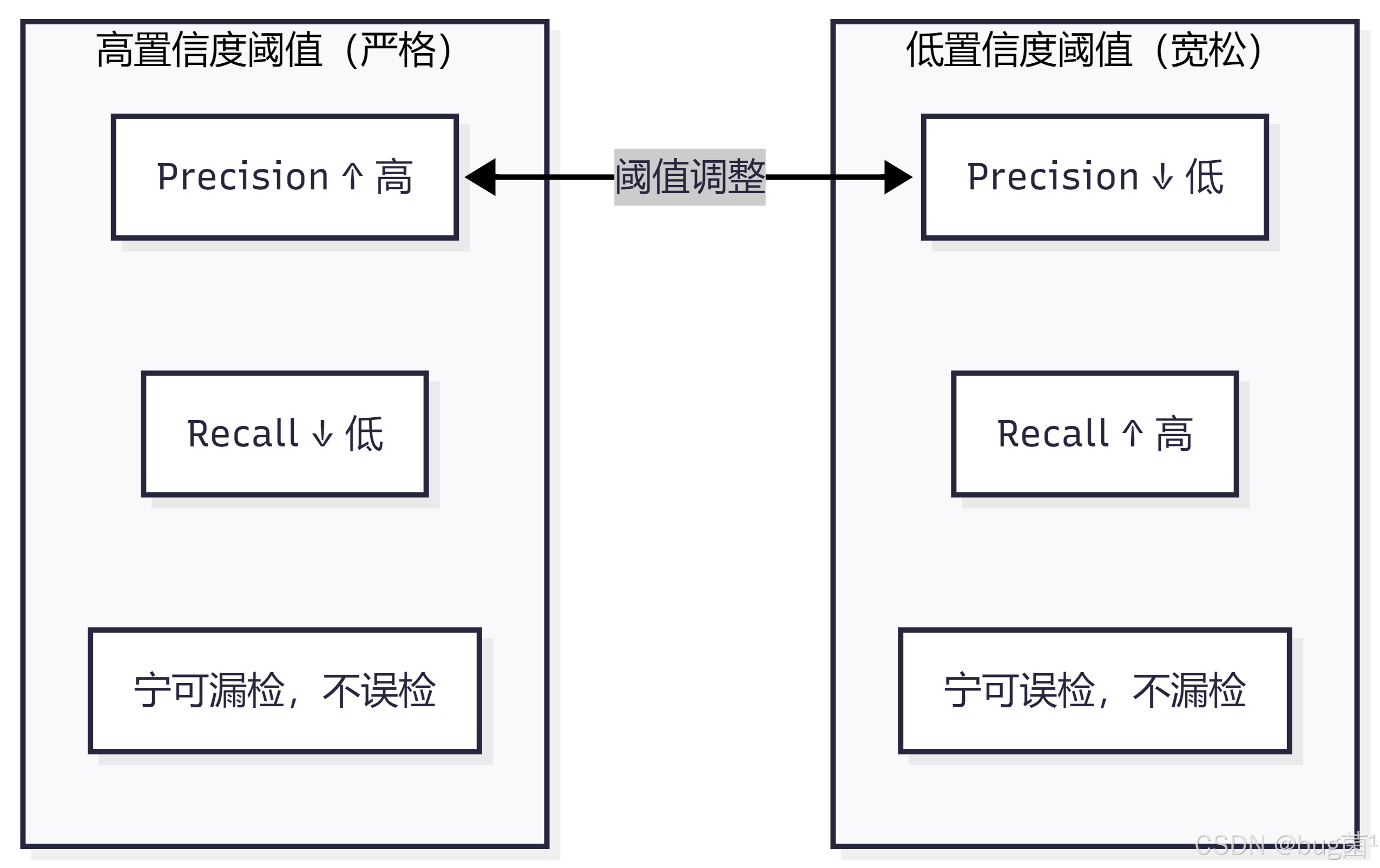
2.3 Precision、Recall 与 F1-Score 深度解析

理解 Precision 和 Recall 的关键在于理解它们的trade-off（权衡关系）。

直觉理解：

• Precision（精确率）：我说检测到的，有多少是真的？——关注误报
• Recall（召回率）：真正存在的目标，我找到了多少？——关注漏报

实际场景中的取舍：

• 🏥 医疗影像检测（漏检代价极大）：更关注 Recall，宁可多检也不漏检
• 🚗 自动驾驶行人检测（两者都重要）：需要平衡 Precision 和 Recall
• 📦 工业质检（误检代价大）：更关注 Precision，减少误报

F1-Score 是 Precision 和 Recall 的调和平均，用于综合评估：

$$F1=\frac{2\times Precision\times Recall}{Precision+Recall}$$

当 Precision = Recall 时，F1 = Precision = Recall，这是最"均衡"的状态。

2.4 PR 曲线与 AP 详解

PR 曲线（Precision-Recall Curve） 是通过改变置信度阈值，描绘 Precision 与 Recall 之间变化关系的曲线。

PR 曲线的生成过程：

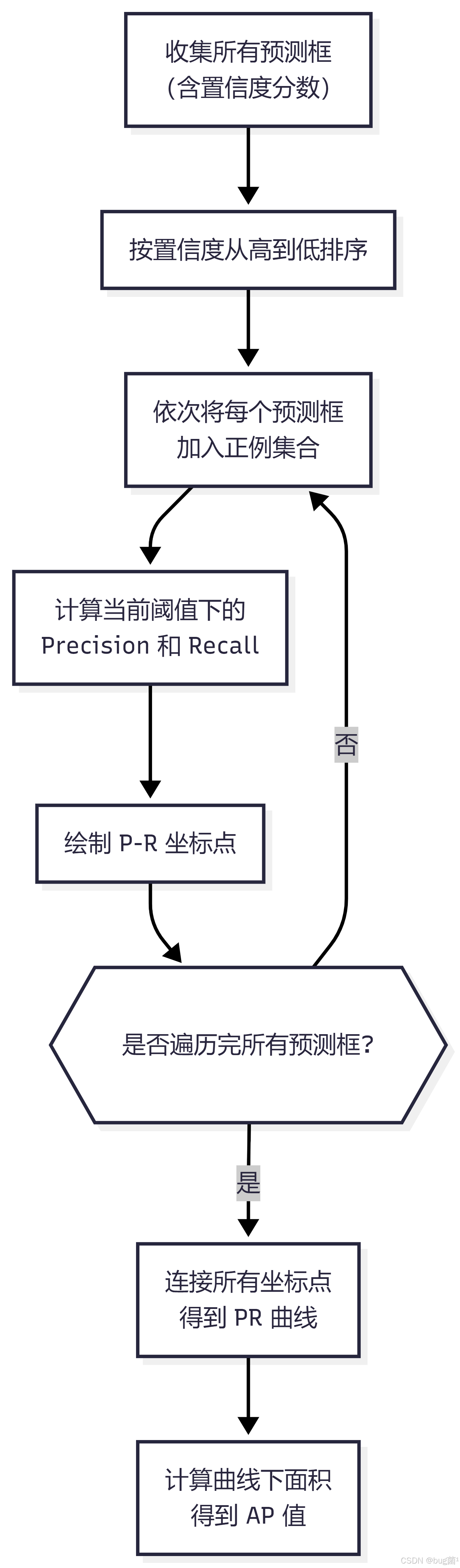
AP（Average Precision，平均精确率） 是 PR 曲线下方的面积，数学上表示为：

$$AP={\int }_0^{1}P(r),dr$$

在实际计算中，通常采用11点插值（PASCAL VOC 2007）或所有点插值（PASCAL VOC 2010+，COCO）。

PR 曲线的解读：

• 曲线越靠近右上角（1,1），模型性能越好
• 曲线下面积（AP）越大越好，最大值为 1.0
• 曲线出现"锯齿"是正常的，因为排序中存在 FP

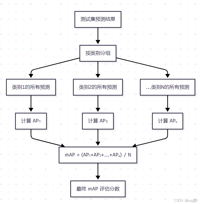
2.5 mAP：目标检测的黄金指标

mAP（mean Average Precision，均值平均精确率） 是目标检测领域最重要的综合评估指标，它对所有类别的 AP 取平均值：

$$mAP=\frac{1}{N}\sum _{i=1}^{N}A{P}_i$$

其中 $N$ 是类别总数，$A{P}_i$ 是第 $i$ 个类别的 AP 值。

mAP 的计算流程图：

2.6 mAP@0.5 vs mAP@0.5:0.95 深度对比

这是 YOLOv11 训练日志中最常见的两个指标，很多初学者对它们的区别一知半解。

指标	全称	IoU 阈值	计算方式	侧重点
mAP@0.5	mAP at IoU=0.50	0.5	单个 IoU 阈值下的 mAP	检测是否正确（粗粒度）
mAP@0.5:0.95	mAP at IoU=0.50:0.05:0.95	0.5, 0.55, …, 0.95（共10个）	10个阈值下 mAP 的平均值	定位精度（细粒度）

mAP@0.5:0.95 的计算：

$$mAP@0.5:0.95=\frac{1}{10}\sum _{t\in 0.5,0.55,0.6,...,0.95}mAP@t$$

💡 选择哪个指标？

• 学术论文、COCO 竞赛：使用 mAP@0.5:0.95（更严格、更全面）
• 工业快速验证：使用 mAP@0.5（直观、计算快）
• 两者都报告是最佳实践

三、YOLOv11 验证流程实战

3.1 val 命令与参数详解

YOLOv11 提供了完善的验证接口，支持 Python API 和 CLI 两种方式。

Python API 验证（推荐）：

# ============================================================
# YOLOv11 模型验证完整示例
# 功能：加载训练好的模型，在验证集上评估性能
# 依赖：ultralytics >= 8.0
# ============================================================

from ultralytics import YOLO
import torch

def run_validation(
    model_path: str,
    data_yaml: str,
    img_size: int = 640,
    batch_size: int = 16,
    conf_threshold: float = 0.001,
    iou_threshold: float = 0.6,
    device: str = None
):
    """
    执行 YOLOv11 模型验证
    
    Args:
        model_path: 训练好的模型权重路径（.pt 文件）
        data_yaml:  数据集配置文件路径（包含 val 路径、类别名称等）
        img_size:   验证时的输入图像尺寸
        batch_size: 验证批次大小（建议 16-32）
        conf_threshold: 置信度阈值（验证时建议设低，如 0.001，让更多框参与计算）
        iou_threshold:  NMS IoU 阈值
        device:     指定设备（None=自动选择，'cpu', '0', '0,1' 等）
    
    Returns:
        results: 包含各项评估指标的结果对象
    """
    
    # 自动检测并选择最优设备
    if device is None:
        device = '0' if torch.cuda.is_available() else 'cpu'
    print(f"🚀 使用设备: {device}")
    
    # 加载模型权重
    # 支持：官方预训练模型名称（如 'yolo11n.pt'）或自定义训练路径
    model = YOLO(model_path)
    print(f"✅ 模型加载成功: {model_path}")
    print(f"   模型类型: {model.info()}")
    
    # 执行验证
    # val() 方法会自动读取 data_yaml 中的 val 路径进行评估
    results = model.val(
        data=data_yaml,          # 数据集配置文件
        imgsz=img_size,          # 输入图像分辨率
        batch=batch_size,        # 批处理大小
        conf=conf_threshold,     # 置信度过滤阈值（验证时设低以获得完整PR曲线）
        iou=iou_threshold,       # NMS IoU 阈值
        device=device,           # 运行设备
        verbose=True,            # 打印详细日志
        save_json=True,          # 保存 COCO 格式 JSON 结果（用于官方评估工具）
        save_hybrid=False,       # 是否保存混合标注（一般不需要）
        plots=True,              # 生成评估可视化图表（PR曲线、混淆矩阵等）
        rect=False,              # 是否使用矩形推理（可加速但影响精度）
        split='val',             # 使用验证集（可选 'test'）
    )
    
    return results


def print_evaluation_report(results):
    """
    格式化打印评估报告
    
    Args:
        results: model.val() 返回的结果对象
    """
    print("\n" + "="*60)
    print("           📊 YOLOv11 模型评估报告")
    print("="*60)
    
    # 整体指标
    # results.box 包含所有检测框相关的评估指标
    box_metrics = results.box
    
    print("\n📌 整体性能指标：")
    print(f"   mAP@0.5        : {box_metrics.map50:.4f}   ({box_metrics.map50*100:.2f}%)")
    print(f"   mAP@0.5:0.95   : {box_metrics.map:.4f}   ({box_metrics.map*100:.2f}%)")
    print(f"   Precision      : {box_metrics.mp:.4f}   ({box_metrics.mp*100:.2f}%)")
    print(f"   Recall         : {box_metrics.mr:.4f}   ({box_metrics.mr*100:.2f}%)")
    
    # 逐类别指标
    print("\n📌 逐类别性能指标：")
    print(f"{'类别':<20} {'Precision':>12} {'Recall':>10} {'AP@0.5':>10} {'AP@.5:.95':>12}")
    print("-" * 66)
    
    # 获取类别名称列表
    names = results.names  # dict: {0: 'person', 1: 'car', ...}
    
    # 遍历每个类别的指标
    # results.box.ap_class_index 包含有效类别的索引
    for i, cls_idx in enumerate(results.box.ap_class_index):
        cls_name = names[cls_idx] if cls_idx in names else f"class_{cls_idx}"
        # ap50: AP at IoU=0.5
        # ap: AP at IoU=0.5:0.95
        ap50 = results.box.ap50[i] if hasattr(results.box, 'ap50') else 0.0
        ap = results.box.ap[i] if hasattr(results.box, 'ap') else 0.0
        # p, r: per-class precision and recall
        p = results.box.p[i] if hasattr(results.box, 'p') else 0.0
        r = results.box.r[i] if hasattr(results.box, 'r') else 0.0
        print(f"  {cls_name:<18} {p:>12.4f} {r:>10.4f} {ap50:>10.4f} {ap:>12.4f}")
    
    print("-" * 66)
    print(f"  {'ALL (mean)':<18} {box_metrics.mp:>12.4f} "
          f"{box_metrics.mr:>10.4f} {box_metrics.map50:>10.4f} {box_metrics.map:>12.4f}")
    
    print("\n" + "="*60)
    print("✅ 评估完成！结果已保存至 runs/val/ 目录")
    print("="*60)


# ---- 主程序入口 ----
if __name__ == "__main__":
    # 示例：验证 COCO 数据集上的 yolo11n 模型
    results = run_validation(
        model_path="yolo11n.pt",          # 模型路径（会自动下载官方预训练模型）
        data_yaml="coco128.yaml",          # 数据集配置（ultralytics 内置示例数据集）
        img_size=640,
        batch_size=16,
        conf_threshold=0.001,             # 验证时置信度尽量低
        iou_threshold=0.6
    )
    
    # 打印格式化报告
    print_evaluation_report(results)

代码解析：

上述代码有几个关键设计值得注意：

1. conf=0.001：验证时置信度阈值要设得很低，这样更多的预测框会参与 PR 曲线的计算，得到的 AP 值更准确。如果阈值设太高（如默认的 0.25），会导致很多低置信度的 TP 被过滤掉，Recall 虚低。

2. save_json=True：保存 COCO 格式的预测结果，可以用官方 pycocotools 进行标准化评估，与其他论文结果对比时更可信。

3. plots=True：自动生成混淆矩阵、PR 曲线、F1 曲线等可视化图表，保存在 runs/val/ 目录下，这是调试的重要工具。

CLI 命令行方式：

# 基础验证命令
yolo val model=yolo11n.pt data=coco128.yaml imgsz=640

# 完整参数验证命令
yolo val \
    model=runs/train/exp/weights/best.pt \
    data=custom_dataset.yaml \
    imgsz=640 \
    batch=16 \
    conf=0.001 \
    iou=0.6 \
    device=0 \
    plots=True \
    save_json=True \
    verbose=True

# 在测试集上评估（注意 split 参数）
yolo val model=best.pt data=custom.yaml split=test

3.2 验证结果解读

运行验证后，YOLOv11 会在终端输出类似以下的结果表格：

                 Class     Images  Instances      P          R      mAP50   mAP50-95
                   all        128        929      0.732      0.665    0.731     0.521
                person        128        254      0.812      0.723    0.805     0.543
                   car        128        116      0.891      0.810    0.873     0.638
               bicycle        128         35      0.654      0.571    0.623     0.412
                ...

字段解析：

字段	含义
Class	类别名称，all 表示所有类别的平均
Images	参与验证的图像数量
Instances	验证集中该类别的真实目标总数
P	Precision（在最优 F1 对应阈值下的精确率）
R	Recall（在最优 F1 对应阈值下的召回率）
mAP50	mAP at IoU=0.5
mAP50-95	mAP at IoU=0.5:0.05:0.95

💡 重要提示：表格中报告的 P 和 R 是在最优置信度阈值（即 F1 最大时对应的阈值）下计算的，并非固定阈值（如 0.5）下的值。这是 YOLOv11/Ultralytics 的计算惯例。

3.3 验证输出文件解读

runs/val/exp/
├── confusion_matrix.png          # 混淆矩阵（归一化）
├── confusion_matrix_normalized.png  # 归一化混淆矩阵
├── PR_curve.png                  # 整体 PR 曲线
├── P_curve.png                   # Precision-Confidence 曲线  
├── R_curve.png                   # Recall-Confidence 曲线
├── F1_curve.png                  # F1-Confidence 曲线（找最优阈值的关键！）
└── predictions.json              # COCO 格式预测结果（save_json=True 时生成）

F1 曲线的重要性：F1_curve.png 横轴是置信度阈值，纵轴是 F1 值。曲线峰值对应的横坐标就是最优置信度阈值，这是模型部署时选择阈值的重要依据。

四、自定义评估指标代码实现

理解评估指标的最好方式是亲手实现它们。下面我们从头手写完整的评估代码，不依赖任何第三方评估库。

4.1 手写 IoU 计算器

# ============================================================
# 文件名：iou_calculator.py
# 功能：实现多种 IoU 变体的计算，包含完整的中文注释
# 支持：标准IoU、GIoU、DIoU、CIoU
# ============================================================

import numpy as np
import torch
import matplotlib.pyplot as plt
import matplotlib.patches as patches


def calculate_iou_numpy(box1: np.ndarray, box2: np.ndarray) -> float:
    """
    计算两个边界框的 IoU（使用 NumPy，适合单对框计算）
    
    Args:
        box1: 格式为 [x1, y1, x2, y2] 的数组（左上角+右下角坐标）
        box2: 格式为 [x1, y1, x2, y2] 的数组
    
    Returns:
        iou: IoU 值，范围 [0, 1]
    
    示例:
        box1 = [100, 100, 300, 300]  # 预测框
        box2 = [150, 150, 350, 350]  # 真实框
        iou = calculate_iou_numpy(box1, box2)  # 约 0.25
    """
    # ---- 第一步：计算交集区域的坐标 ----
    # 交集左上角 = 两框左上角的最大值（取更靠右下的那个）
    inter_x1 = max(box1[0], box2[0])
    inter_y1 = max(box1[1], box2[1])
    # 交集右下角 = 两框右下角的最小值（取更靠左上的那个）
    inter_x2 = min(box1[2], box2[2])
    inter_y2 = min(box1[3], box2[3])
    
    # ---- 第二步：计算交集面积 ----
    # 如果 inter_x2 <= inter_x1 或 inter_y2 <= inter_y1，说明两框不相交
    inter_w = max(0, inter_x2 - inter_x1)  # 交集宽度，不能为负
    inter_h = max(0, inter_y2 - inter_y1)  # 交集高度，不能为负
    inter_area = inter_w * inter_h
    
    # ---- 第三步：计算各自面积 ----
    area1 = (box1[2] - box1[0]) * (box1[3] - box1[1])  # 预测框面积
    area2 = (box2[2] - box2[0]) * (box2[3] - box2[1])  # 真实框面积
    
    # ---- 第四步：计算并集面积（避免重复计算交集）----
    union_area = area1 + area2 - inter_area
    
    # ---- 第五步：计算 IoU，添加极小值避免除零 ----
    iou = inter_area / (union_area + 1e-7)
    
    return iou


def calculate_iou_batch(boxes1: torch.Tensor, boxes2: torch.Tensor) -> torch.Tensor:
    """
    批量计算两组边界框之间的 IoU 矩阵（使用 PyTorch，GPU加速）
    
    Args:
        boxes1: shape [N, 4]，格式 [x1, y1, x2, y2]
        boxes2: shape [M, 4]，格式 [x1, y1, x2, y2]
    
    Returns:
        iou_matrix: shape [N, M]，boxes1[i] 与 boxes2[j] 的 IoU 值
    
    注意：
        使用广播机制实现向量化计算，避免 Python 循环，效率极高
    """
    # 扩维以支持广播：[N,4] -> [N,1,4]，[M,4] -> [1,M,4]
    boxes1 = boxes1.unsqueeze(1)  # [N, 1, 4]
    boxes2 = boxes2.unsqueeze(0)  # [1, M, 4]
    
    # 计算交集坐标（广播后自动对所有 N×M 对进行计算）
    inter_x1 = torch.max(boxes1[..., 0], boxes2[..., 0])  # [N, M]
    inter_y1 = torch.max(boxes1[..., 1], boxes2[..., 1])
    inter_x2 = torch.min(boxes1[..., 2], boxes2[..., 2])
    inter_y2 = torch.min(boxes1[..., 3], boxes2[..., 3])
    
    # 计算交集面积（clamp 保证非负）
    inter_w = (inter_x2 - inter_x1).clamp(min=0)
    inter_h = (inter_y2 - inter_y1).clamp(min=0)
    inter_area = inter_w * inter_h  # [N, M]
    
    # 计算各自面积
    area1 = ((boxes1[..., 2] - boxes1[..., 0]) * 
             (boxes1[..., 3] - boxes1[..., 1]))  # [N, 1]
    area2 = ((boxes2[..., 2] - boxes2[..., 0]) * 
             (boxes2[..., 3] - boxes2[..., 1]))  # [1, M]
    
    # 并集面积
    union_area = area1 + area2 - inter_area  # [N, M]
    
    # IoU 矩阵
    iou_matrix = inter_area / (union_area + 1e-7)
    
    return iou_matrix


def visualize_iou(box1, box2, iou_value):
    """
    可视化两个边界框及其 IoU
    
    Args:
        box1: [x1, y1, x2, y2] 预测框坐标
        box2: [x1, y1, x2, y2] 真实框坐标
        iou_value: 已计算的 IoU 值
    """
    fig, ax = plt.subplots(1, 1, figsize=(7, 6))
    ax.set_xlim(0, 500)
    ax.set_ylim(0, 500)
    ax.invert_yaxis()  # 图像坐标系 y 轴向下
    
    # 绘制预测框（蓝色）
    pred_rect = patches.Rectangle(
        (box1[0], box1[1]),
        box1[2] - box1[0], box1[3] - box1[1],
        linewidth=2, edgecolor='blue', facecolor='blue', alpha=0.2,
        label=f'Predicted Box'
    )
    ax.add_patch(pred_rect)
    
    # 绘制真实框（绿色）
    gt_rect = patches.Rectangle(
        (box2[0], box2[1]),
        box2[2] - box2[0], box2[3] - box2[1],
        linewidth=2, edgecolor='green', facecolor='green', alpha=0.2,
        label=f'Ground Truth Box'
    )
    ax.add_patch(gt_rect)
    
    # 绘制交集框（红色）
    inter_x1 = max(box1[0], box2[0])
    inter_y1 = max(box1[1], box2[1])
    inter_x2 = min(box1[2], box2[2])
    inter_y2 = min(box1[3], box2[3])
    
    if inter_x2 > inter_x1 and inter_y2 > inter_y1:
        inter_rect = patches.Rectangle(
            (inter_x1, inter_y1),
            inter_x2 - inter_x1, inter_y2 - inter_y1,
            linewidth=2, edgecolor='red', facecolor='red', alpha=0.4,
            label='Intersection'
        )
        ax.add_patch(inter_rect)
    
    ax.set_title(f'IoU Visualization\nIoU = {iou_value:.4f}', fontsize=14, fontweight='bold')
    ax.legend(fontsize=11)
    ax.set_xlabel('X Coordinate')
    ax.set_ylabel('Y Coordinate')
    ax.grid(True, alpha=0.3)
    plt.tight_layout()
    plt.savefig('iou_visualization.png', dpi=150, bbox_inches='tight')
    plt.show()
    print("✅ IoU 可视化图已保存：iou_visualization.png")


# ---- 单元测试 ----
if __name__ == "__main__":
    print("=" * 50)
    print("   IoU 计算器测试")
    print("=" * 50)
    
    # 测试用例1：部分重叠
    box_pred = np.array([100, 100, 300, 300])  # 预测框
    box_gt   = np.array([150, 150, 350, 350])  # 真实框
    iou = calculate_iou_numpy(box_pred, box_gt)
    print(f"\n测试1 - 部分重叠:")
    print(f"  预测框: {box_pred}")
    print(f"  真实框: {box_gt}")
    print(f"  IoU = {iou:.4f}（约 0.25，交集面积150²=22500，并集=60000-22500+60000=90000）")
    
    # 测试用例2：完全包含
    box_pred2 = np.array([50, 50, 400, 400])
    box_gt2   = np.array([100, 100, 300, 300])
    iou2 = calculate_iou_numpy(box_pred2, box_gt2)
    print(f"\n测试2 - 预测框包含真实框:")
    print(f"  IoU = {iou2:.4f}")
    
    # 测试用例3：完全不重叠
    box_pred3 = np.array([0, 0, 100, 100])
    box_gt3   = np.array([200, 200, 300, 300])
    iou3 = calculate_iou_numpy(box_pred3, box_gt3)
    print(f"\n测试3 - 完全不重叠:")
    print(f"  IoU = {iou3:.4f}（期望: 0.0000）")
    
    # 测试用例4：批量 IoU 矩阵
    print("\n测试4 - 批量 IoU 矩阵（2个预测框 vs 3个真实框）:")
    preds = torch.tensor([[100,100,300,300], [200,200,400,400]], dtype=torch.float32)
    gts   = torch.tensor([[150,150,350,350], [50,50,250,250], [250,250,450,450]], dtype=torch.float32)
    iou_matrix = calculate_iou_batch(preds, gts)
    print(f"  IoU 矩阵 (shape: {iou_matrix.shape}):\n{iou_matrix}")
    
    # 可视化
    visualize_iou(box_pred.tolist(), box_gt.tolist(), iou)

代码解析：

• calculate_iou_numpy 使用纯 NumPy 逐步计算，逻辑清晰，适合教学和理解原理。
• calculate_iou_batch 使用 PyTorch 广播机制，一次性计算 N×M 个 IoU 值，这是 YOLOv11 内部 NMS 和 mAP 计算的核心技术。理解广播机制是掌握深度学习矩阵运算的关键。
• clamp(min=0) 用于处理不相交情况（交集宽高为负数的边界情况）。

4.2 手写 PR 曲线与 AP 计算

# ============================================================
# 文件名：pr_curve_calculator.py  
# 功能：从预测结果手动计算 PR 曲线和 AP 值
# 方法：所有点插值（VOC 2010+，与 COCO 标准一致）
# ============================================================

import numpy as np
import matplotlib.pyplot as plt
from typing import List, Tuple


def compute_ap_from_pr(recalls: np.ndarray, precisions: np.ndarray) -> float:
    """
    从 PR 曲线计算 AP（使用所有点插值法，VOC 2010+）
    
    核心思想：对 PR 曲线进行单调递减处理后，计算曲线下面积
    
    Args:
        recalls:    召回率数组（从小到大排列）
        precisions: 精确率数组（对应每个召回率值）
    
    Returns:
        ap: Average Precision 值，范围 [0, 1]
    
    算法步骤：
        1. 在两端补 0（使曲线从原点出发，延伸到 recall=1.0）
        2. 对 precision 做单调递减处理（取右侧最大值，消除锯齿）
        3. 找到 recall 变化的位置，用矩形面积近似计算曲线下面积
    """
    # 步骤1：在首尾补充边界点，确保 PR 曲线起点和终点正确
    # np.concatenate 拼接数组
    recalls_ext    = np.concatenate([[0.0], recalls, [1.0]])
    precisions_ext = np.concatenate([[1.0], precisions, [0.0]])
    
    # 步骤2：单调递减处理（从右往左取最大值）
    # np.maximum.accumulate 是累积最大值操作
    # [::-1] 表示数组翻转（从右到左）
    precisions_ext = np.maximum.accumulate(precisions_ext[::-1])[::-1]
    
    # 步骤3：找 recall 发生变化的位置
    # np.diff 计算相邻元素之差
    # np.where 返回满足条件的索引
    change_points = np.where(np.diff(recalls_ext) != 0)[0]
    
    # 步骤4：用矩形面积近似 PR 曲线下面积
    # 每个矩形的宽 = recall 的变化量（delta_r）
    # 每个矩形的高 = 该位置的 precision 值
    ap = np.sum(
        (recalls_ext[change_points + 1] - recalls_ext[change_points]) * 
        precisions_ext[change_points + 1]
    )
    
    return float(ap)


def compute_pr_curve(
    pred_scores: np.ndarray,      # 每个预测框的置信度分数
    pred_labels: np.ndarray,      # 每个预测框的预测类别
    pred_boxes:  np.ndarray,      # 每个预测框的坐标 [N, 4]
    gt_labels:   List[np.ndarray],# 每张图的真实类别列表
    gt_boxes:    List[np.ndarray],# 每张图的真实框坐标列表
    target_class: int,            # 要计算 AP 的目标类别 ID
    iou_threshold: float = 0.5    # IoU 阈值
) -> Tuple[np.ndarray, np.ndarray, float]:
    """
    计算指定类别的 PR 曲线和 AP 值
    
    Args:
        pred_scores:   预测置信度数组，shape [N]
        pred_labels:   预测类别数组，shape [N]
        pred_boxes:    预测框坐标数组，shape [N, 4]，格式 [x1,y1,x2,y2]
        gt_labels:     真实类别列表，每个元素对应一张图片的标注
        gt_boxes:      真实框坐标列表，每个元素对应一张图片的标注
        target_class:  目标类别 ID
        iou_threshold: 判断 TP 的 IoU 阈值
    
    Returns:
        recalls:    召回率数组
        precisions: 精确率数组
        ap:         AP 值
    """
    
    # ---- 第一步：统计该类别的真实目标总数 ----
    total_gt = sum(
        np.sum(labels == target_class) 
        for labels in gt_labels
    )
    
    if total_gt == 0:
        print(f"⚠️ 类别 {target_class} 没有真实目标，AP=0")
        return np.array([0.0]), np.array([0.0]), 0.0
    
    # ---- 第二步：筛选该类别的预测框 ----
    # 找到预测类别等于目标类别的预测框
    class_mask = (pred_labels == target_class)
    cls_scores = pred_scores[class_mask]   # 筛选后的置信度
    cls_boxes  = pred_boxes[class_mask]    # 筛选后的预测框坐标
    
    if len(cls_scores) == 0:
        # 没有任何预测框，召回率为0
        return np.array([0.0]), np.array([0.0]), 0.0
    
    # ---- 第三步：按置信度从高到低排序 ----
    sorted_indices = np.argsort(-cls_scores)  # 降序排列
    cls_scores = cls_scores[sorted_indices]
    cls_boxes  = cls_boxes[sorted_indices]
    
    # ---- 第四步：逐一判断每个预测框是 TP 还是 FP ----
    tp_list = []  # 存储每个预测框是否为 TP（1）或 FP（0）
    
    # 记录每张图片中已被匹配的真实框（防止一个 GT 被多次匹配）
    # gt_matched[img_idx][gt_idx] = True 表示该 GT 已被匹配
    gt_matched = [
        np.zeros(np.sum(labels == target_class), dtype=bool)
        for labels in gt_labels
    ]
    
    # 注意：这里简化处理，假设所有预测都来自同一张图
    # 实际使用时需要每个预测框关联到其所属图片 ID
    # 为演示目的，此处对全部预测框与全部 GT 框做匹配
    all_gt_boxes = np.concatenate(
        [boxes[labels == target_class] for boxes, labels in zip(gt_boxes, gt_labels)]
        if any(np.sum(labels == target_class) > 0 for labels in gt_labels)
        else [np.empty((0, 4))]
    )
    all_gt_matched = np.zeros(len(all_gt_boxes), dtype=bool)
    
    for pred_box in cls_boxes:
        if len(all_gt_boxes) == 0:
            # 没有真实框，全部预测为 FP
            tp_list.append(0)
            continue
        
        # 计算该预测框与所有真实框的 IoU
        ious = np.array([
            calculate_iou_numpy(pred_box, gt_box) 
            for gt_box in all_gt_boxes
        ])
        
        # 找最大 IoU 对应的真实框
        max_iou_idx = np.argmax(ious)
        max_iou     = ious[max_iou_idx]
        
        if max_iou >= iou_threshold and not all_gt_matched[max_iou_idx]:
            # 满足条件且该 GT 尚未被匹配 → TP
            tp_list.append(1)
            all_gt_matched[max_iou_idx] = True
        else:
            # IoU 不足或 GT 已被匹配 → FP
            tp_list.append(0)
    
    # ---- 第五步：计算累积 TP 和 FP ----
    tp_array = np.array(tp_list)
    cumulative_tp = np.cumsum(tp_array)          # 累积 TP 数量
    cumulative_fp = np.cumsum(1 - tp_array)      # 累积 FP 数量
    
    # ---- 第六步：计算 Precision 和 Recall ----
    recalls    = cumulative_tp / (total_gt + 1e-7)
    precisions = cumulative_tp / (cumulative_tp + cumulative_fp + 1e-7)
    
    # ---- 第七步：计算 AP ----
    ap = compute_ap_from_pr(recalls, precisions)
    
    return recalls, precisions, ap


def plot_pr_curve(recalls, precisions, ap, class_name="Object", save_path=None):
    """
    绘制 PR 曲线
    
    Args:
        recalls:    召回率数组
        precisions: 精确率数组
        ap:         AP 值（用于标注在图表上）
        class_name: 类别名称
        save_path:  保存路径（为 None 则直接显示）
    """
    plt.figure(figsize=(8, 6))
    
    # 绘制 PR 曲线
    plt.step(recalls, precisions, color='royalblue', alpha=0.8, 
             where='post', linewidth=2, label=f'PR Curve (AP={ap:.4f})')
    
    # 填充曲线下面积
    plt.fill_between(recalls, precisions, alpha=0.15, color='royalblue', step='post')
    
    # 标注 AP 值
    plt.annotate(
        f'AP = {ap:.4f}',
        xy=(0.6, 0.8), fontsize=13, color='darkblue',
        bbox=dict(boxstyle='round,pad=0.3', facecolor='lightyellow', edgecolor='gray')
    )
    
    plt.xlabel('Recall', fontsize=13)
    plt.ylabel('Precision', fontsize=13)
    plt.title(f'Precision-Recall Curve - Class: {class_name}', fontsize=14, fontweight='bold')
    plt.xlim([0.0, 1.05])
    plt.ylim([0.0, 1.05])
    plt.legend(fontsize=12)
    plt.grid(True, alpha=0.3)
    plt.tight_layout()
    
    if save_path:
        plt.savefig(save_path, dpi=150, bbox_inches='tight')
        print(f"✅ PR 曲线已保存：{save_path}")
    plt.show()


# ---- 辅助函数（复用上一节的计算） ----
def calculate_iou_numpy(box1, box2):
    """简化版 IoU 计算（复用函数）"""
    ix1, iy1 = max(box1[0], box2[0]), max(box1[1], box2[1])
    ix2, iy2 = min(box1[2], box2[2]), min(box1[3], box2[3])
    inter = max(0, ix2-ix1) * max(0, iy2-iy1)
    a1 = (box1[2]-box1[0]) * (box1[3]-box1[1])
    a2 = (box2[2]-box2[0]) * (box2[3]-box2[1])
    return inter / (a1 + a2 - inter + 1e-7)


# ---- 模拟测试 ----
if __name__ == "__main__":
    np.random.seed(42)  # 固定随机种子，确保可复现
    
    print("=" * 55)
    print("   PR 曲线与 AP 计算演示（类别0 = 'person'）")
    print("=" * 55)
    
    # 模拟生成预测框：10个预测，包含不同置信度和不同类别
    n_preds = 10
    pred_scores = np.array([0.95, 0.88, 0.82, 0.75, 0.68, 0.60, 0.55, 0.48, 0.35, 0.20])
    pred_labels = np.array([0, 0, 1, 0, 0, 1, 0, 0, 1, 0])  # 0=person，1=car
    pred_boxes  = np.array([
        [100, 100, 300, 350],  # 置信度 0.95，与 GT0 重叠高 → TP
        [200, 150, 380, 400],  # 置信度 0.88，与 GT1 重叠高 → TP
        [50,  50,  200, 200],  # 置信度 0.82，car 类
        [100, 100, 310, 360],  # 置信度 0.75，与 GT0 重叠但 GT0 已匹配 → FP（重复）
        [400, 400, 500, 500],  # 置信度 0.68，无对应 GT → FP（误检）
        [150, 150, 320, 380],  # 置信度 0.60，car 类
        [210, 160, 375, 395],  # 置信度 0.55，与 GT1 重叠，但 GT1 已匹配 → FP
        [10,  10,  120, 150],  # 置信度 0.48，无对应 GT → FP（误检）
        [300, 300, 450, 480],  # 置信度 0.35，car 类
        [190, 140, 370, 390],  # 置信度 0.20，与 GT1 重叠，但已匹配 → FP
    ], dtype=float)
    
    # 模拟真实标注（假设只有一张图片，两个 person 目标）
    gt_labels = [np.array([0, 0])]  # 两个 person
    gt_boxes  = [np.array([
        [105, 105, 298, 345],  # GT0：person
        [205, 155, 375, 398],  # GT1：person
    ], dtype=float)]
    
    # 计算 person 类（class_id=0）的 PR 曲线和 AP
    recalls, precisions, ap = compute_pr_curve(
        pred_scores, pred_labels, pred_boxes,
        gt_labels, gt_boxes,
        target_class=0,
        iou_threshold=0.5
    )
    
    print(f"\n📊 PR 曲线数据点（前10个）:")
    print(f"  {'Recall':>10}  {'Precision':>12}")
    print("  " + "-"*25)
    for r, p in zip(recalls[:10], precisions[:10]):
        print(f"  {r:>10.4f}  {p:>12.4f}")
    
    print(f"\n🎯 AP@0.5 = {ap:.4f}  ({ap*100:.2f}%)")
    
    # 绘制 PR 曲线
    plot_pr_curve(recalls, precisions, ap, class_name='person', 
                  save_path='pr_curve_person.png')

代码解析：

1. compute_ap_from_pr 的核心技巧：单调递减处理（np.maximum.accumulate）是消除 PR 曲线锯齿的关键步骤。在实际排序过程中，遇到 FP 时 Precision 会下降，但标准 AP 计算规定：某个 Recall 值处的 Precision 应取该 Recall 值之后所有点中 Precision 的最大值。

2. GT 匹配防止重复：all_gt_matched 数组记录已被匹配的真实框，确保一个 GT 只能匹配一个预测框（取置信度最高的）。这是目标检测评估与图像分类评估的重要区别。

3. np.cumsum：累积求和是高效计算累积 TP/FP 的关键操作，避免了低效的循环计算。

4.3 手写完整 mAP 计算器

# ============================================================
# 文件名：map_calculator.py
# 功能：完整的 mAP 计算器，支持 mAP@0.5 和 mAP@0.5:0.95
# 适用：PASCAL VOC / COCO 风格的目标检测评估
# ============================================================

import numpy as np
import matplotlib.pyplot as plt
from collections import defaultdict
from typing import Dict, List, Tuple


class DetectionEvaluator:
    """
    目标检测完整评估器
    支持多类别、多图片、多 IoU 阈值的 mAP 计算
    
    使用示例:
        evaluator = DetectionEvaluator(num_classes=3, 
                                        class_names=['cat','dog','bird'])
        # 逐张图片添加预测和真实标注
        evaluator.add_predictions(image_id=0, pred_boxes=..., pred_scores=..., pred_classes=...)
        evaluator.add_ground_truths(image_id=0, gt_boxes=..., gt_classes=...)
        # 计算 mAP
        results = evaluator.compute_map()
    """
    
    def __init__(self, num_classes: int, class_names: List[str] = None):
        """
        初始化评估器
        
        Args:
            num_classes: 类别总数
            class_names: 类别名称列表（可选，用于打印报告）
        """
        self.num_classes = num_classes
        self.class_names = class_names or [f'class_{i}' for i in range(num_classes)]
        
        # 存储所有图片的预测结果
        # 格式：{image_id: {'boxes': [...], 'scores': [...], 'classes': [...]}}
        self.predictions: Dict = defaultdict(lambda: {'boxes': [], 'scores': [], 'classes': []})
        
        # 存储所有图片的真实标注
        # 格式：{image_id: {'boxes': [...], 'classes': [...]}}
        self.ground_truths: Dict = defaultdict(lambda: {'boxes': [], 'classes': []})
        
        self.image_ids = set()  # 已添加数据的图片 ID 集合
    
    def add_predictions(
        self, 
        image_id: int, 
        pred_boxes: np.ndarray,   # shape [N, 4]，格式 [x1,y1,x2,y2]
        pred_scores: np.ndarray,  # shape [N]，置信度
        pred_classes: np.ndarray  # shape [N]，预测类别 ID
    ):
        """添加一张图片的预测结果"""
        self.predictions[image_id]['boxes']   = np.array(pred_boxes,   dtype=float)
        self.predictions[image_id]['scores']  = np.array(pred_scores,  dtype=float)
        self.predictions[image_id]['classes'] = np.array(pred_classes, dtype=int)
        self.image_ids.add(image_id)
    
    def add_ground_truths(
        self, 
        image_id: int, 
        gt_boxes: np.ndarray,    # shape [M, 4]，格式 [x1,y1,x2,y2]
        gt_classes: np.ndarray   # shape [M]，真实类别 ID
    ):
        """添加一张图片的真实标注"""
        self.ground_truths[image_id]['boxes']   = np.array(gt_boxes,   dtype=float)
        self.ground_truths[image_id]['classes'] = np.array(gt_classes, dtype=int)
        self.image_ids.add(image_id)
    
    def _compute_iou(self, box1: np.ndarray, box2: np.ndarray) -> float:
        """计算两个框的 IoU（内部方法）"""
        ix1, iy1 = max(box1[0], box2[0]), max(box1[1], box2[1])
        ix2, iy2 = min(box1[2], box2[2]), min(box1[3], box2[3])
        inter = max(0.0, ix2-ix1) * max(0.0, iy2-iy1)
        a1 = (box1[2]-box1[0]) * (box1[3]-box1[1])
        a2 = (box2[2]-box2[0]) * (box2[3]-box2[1])
        return inter / (a1 + a2 - inter + 1e-9)
    
    def _compute_ap_for_class(
        self, 
        class_id: int, 
        iou_threshold: float
    ) -> Tuple[np.ndarray, np.ndarray, float]:
        """
        计算单个类别在指定 IoU 阈值下的 AP
        
        核心流程：
        1. 收集该类别在所有图片中的预测框，按置信度排序
        2. 逐一与对应图片的 GT 框匹配（使用 IoU 阈值判定 TP/FP）
        3. 计算累积 PR，调用 AP 计算函数
        """
        
        # ---- 收集所有图片中该类别的预测框 ----
        all_preds = []  # 每个元素：(image_id, score, box)
        
        for img_id in self.image_ids:
            pred = self.predictions[img_id]
            if len(pred['classes']) == 0:
                continue
            
            # 筛选当前类别的预测
            cls_mask = (pred['classes'] == class_id)
            cls_scores = pred['scores'][cls_mask]
            cls_boxes  = pred['boxes'][cls_mask] if len(pred['boxes']) > 0 else np.empty((0, 4))
            
            for score, box in zip(cls_scores, cls_boxes):
                all_preds.append((img_id, float(score), box))
        
        # ---- 统计该类别的真实框总数 ----
        total_gt = 0
        for img_id in self.image_ids:
            gt = self.ground_truths[img_id]
            if len(gt['classes']) > 0:
                total_gt += int(np.sum(gt['classes'] == class_id))
        
        if total_gt == 0:
            return np.array([0.0]), np.array([1.0]), 0.0
        
        if len(all_preds) == 0:
            return np.array([0.0]), np.array([0.0]), 0.0
        
        # ---- 按置信度从高到低排序 ----
        all_preds.sort(key=lambda x: -x[1])
        
        # ---- 记录每张图片 GT 的匹配状态 ----
        # gt_matched_status[img_id] 是长度等于该图片该类别 GT 数量的布尔数组
        gt_matched_status = {}
        for img_id in self.image_ids:
            gt = self.ground_truths[img_id]
            if len(gt['classes']) > 0:
                n_cls_gt = int(np.sum(gt['classes'] == class_id))
                gt_matched_status[img_id] = np.zeros(n_cls_gt, dtype=bool)
        
        # ---- 逐一判断 TP / FP ----
        tp_arr = np.zeros(len(all_preds))
        fp_arr = np.zeros(len(all_preds))
        
        for pred_idx, (img_id, score, pred_box) in enumerate(all_preds):
            gt = self.ground_truths[img_id]
            
            if len(gt['classes']) == 0:
                fp_arr[pred_idx] = 1  # 该图片无 GT → FP
                continue
            
            # 获取该图片中该类别的所有 GT 框
            cls_gt_mask  = (gt['classes'] == class_id)
            cls_gt_boxes = gt['boxes'][cls_gt_mask] if len(gt['boxes']) > 0 else np.empty((0, 4))
            
            if len(cls_gt_boxes) == 0:
                fp_arr[pred_idx] = 1  # 该图片无该类别 GT → FP
                continue
            
            # 计算与所有 GT 的 IoU，找最大匹配
            ious = np.array([self._compute_iou(pred_box, gt_box) for gt_box in cls_gt_boxes])
            best_match_idx = int(np.argmax(ious))
            best_iou       = ious[best_match_idx]
            
            matched_status = gt_matched_status.get(img_id, np.array([]))
            
            if (best_iou >= iou_threshold and 
                len(matched_status) > best_match_idx and 
                not matched_status[best_match_idx]):
                # 匹配成功，标记为 TP，并将该 GT 置为已匹配
                tp_arr[pred_idx] = 1
                gt_matched_status[img_id][best_match_idx] = True
            else:
                # IoU 不足或 GT 已匹配 → FP
                fp_arr[pred_idx] = 1
        
        # ---- 计算累积 TP/FP 和 PR 曲线 ----
        cum_tp = np.cumsum(tp_arr)
        cum_fp = np.cumsum(fp_arr)
        
        recalls    = cum_tp / (total_gt + 1e-9)
        precisions = cum_tp / (cum_tp + cum_fp + 1e-9)
        
        # ---- 计算 AP ----
        # 在首尾补充边界点
        r_full = np.concatenate([[0.0], recalls,    [1.0]])
        p_full = np.concatenate([[1.0], precisions, [0.0]])
        
        # 单调递减处理
        p_full = np.maximum.accumulate(p_full[::-1])[::-1]
        
        # 计算面积
        change_pts = np.where(np.diff(r_full) != 0)[0]
        ap = float(np.sum((r_full[change_pts+1] - r_full[change_pts]) * p_full[change_pts+1]))
        
        return recalls, precisions, ap
    
    def compute_map(
        self, 
        iou_thresholds: List[float] = None
    ) -> Dict:
        """
        计算完整的 mAP 报告
        
        Args:
            iou_thresholds: IoU 阈值列表
                           默认：[0.5]（mAP@0.5）
                           COCO：[0.5, 0.55, 0.6, ..., 0.95]（mAP@0.5:0.95）
        
        Returns:
            results: 包含 per-class AP、mAP@0.5、mAP@0.5:0.95 等指标的字典
        """
        if iou_thresholds is None:
            # 默认使用 COCO 标准（10个 IoU 阈值）
            iou_thresholds = np.arange(0.5, 1.0, 0.05).tolist()  # [0.5, 0.55, ..., 0.95]
        
        results = {
            'per_class_ap50':      {},   # 每个类别的 AP@0.5
            'per_class_ap50_95':   {},   # 每个类别的 AP@0.5:0.95
            'per_class_pr_curves': {},   # 每个类别的 PR 曲线数据
            'map50':    0.0,             # 整体 mAP@0.5
            'map50_95': 0.0,             # 整体 mAP@0.5:0.95
        }
        
        all_ap50     = []
        all_ap50_95  = []
        
        for class_id in range(self.num_classes):
            class_name = self.class_names[class_id]
            
            # 计算 AP@0.5
            recalls, precisions, ap50 = self._compute_ap_for_class(class_id, iou_threshold=0.5)
            results['per_class_ap50'][class_name]      = ap50
            results['per_class_pr_curves'][class_name] = (recalls, precisions)
            all_ap50.append(ap50)
            
            # 计算 AP@0.5:0.95（对多个 IoU 阈值取平均）
            ap_per_threshold = []
            for iou_t in iou_thresholds:
                _, _, ap_t = self._compute_ap_for_class(class_id, iou_threshold=iou_t)
                ap_per_threshold.append(ap_t)
            ap50_95 = float(np.mean(ap_per_threshold))
            results['per_class_ap50_95'][class_name] = ap50_95
            all_ap50_95.append(ap50_95)
        
        # 计算整体 mAP（对所有类别取平均）
        results['map50']    = float(np.mean(all_ap50))
        results['map50_95'] = float(np.mean(all_ap50_95))
        
        return results
    
    def print_report(self, results: Dict):
        """打印格式化评估报告"""
        print("\n" + "="*68)
        print("              🎯 目标检测 mAP 评估报告")
        print("="*68)
        print(f"\n{'类别名称':<20} {'AP@0.5':>12} {'AP@0.5:0.95':>14}")
        print("-" * 48)
        
        for class_name in self.class_names:
            ap50    = results['per_class_ap50'].get(class_name, 0.0)
            ap50_95 = results['per_class_ap50_95'].get(class_name, 0.0)
            print(f"  {class_name:<18} {ap50:>12.4f} {ap50_95:>14.4f}")
        
        print("-" * 48)
        print(f"  {'ALL (mAP)':<18} {results['map50']:>12.4f} {results['map50_95']:>14.4f}")
        print("\n" + "="*68)
        print(f"  ✅ mAP@0.5        = {results['map50']:.4f} ({results['map50']*100:.2f}%)")
        print(f"  ✅ mAP@0.5:0.95   = {results['map50_95']:.4f} ({results['map50_95']*100:.2f}%)")
        print("="*68)
    
    def plot_all_pr_curves(self, results: Dict, save_path: str = None):
        """绘制所有类别的 PR 曲线（多子图）"""
        n_cls = self.num_classes
        cols  = min(3, n_cls)
        rows  = (n_cls + cols - 1) // cols
        
        fig, axes = plt.subplots(rows, cols, figsize=(5*cols, 4*rows))
        axes = axes.flatten() if n_cls > 1 else [axes]
        
        colors = plt.cm.Set2(np.linspace(0, 1, n_cls))
        
        for i, class_name in enumerate(self.class_names):
            ax = axes[i]
            recalls, precisions = results['per_class_pr_curves'][class_name]
            ap50 = results['per_class_ap50'][class_name]
            
            ax.step(recalls, precisions, color=colors[i], alpha=0.9, 
                    where='post', linewidth=2)
            ax.fill_between(recalls, precisions, alpha=0.15, 
                            color=colors[i], step='post')
            ax.set_title(f'{class_name}\nAP@0.5={ap50:.3f}', fontsize=11, fontweight='bold')
            ax.set_xlabel('Recall', fontsize=10)
            ax.set_ylabel('Precision', fontsize=10)
            ax.set_xlim([0.0, 1.05])
            ax.set_ylim([0.0, 1.05])
            ax.grid(True, alpha=0.3)
        
        # 隐藏多余的子图
        for j in range(n_cls, len(axes)):
            axes[j].set_visible(False)
        
        # 添加总标题
        fig.suptitle(
            f'PR Curves for All Classes\n'
            f'mAP@0.5={results["map50"]:.4f}  |  mAP@0.5:0.95={results["map50_95"]:.4f}',
            fontsize=13, fontweight='bold', y=1.02
        )
        
        plt.tight_layout()
        if save_path:
            plt.savefig(save_path, dpi=150, bbox_inches='tight')
            print(f"✅ 所有类别 PR 曲线已保存：{save_path}")
        plt.show()


# ===================== 主程序测试 =====================
if __name__ == "__main__":
    np.random.seed(2024)
    
    print("=" * 60)
    print("   完整 mAP 计算器演示（3类别 × 5张图片）")
    print("=" * 60)
    
    # 初始化评估器
    evaluator = DetectionEvaluator(
        num_classes=3,
        class_names=['cat', 'dog', 'bird']
    )
    
    # ---- 模拟 5 张图片的标注和预测 ----
    # 图片0：包含1只猫、1只狗
    evaluator.add_ground_truths(
        image_id=0,
        gt_boxes=np.array([[50,50,200,200],[250,100,400,300]], dtype=float),
        gt_classes=np.array([0, 1])  # cat, dog
    )
    evaluator.add_predictions(
        image_id=0,
        pred_boxes=np.array([[55,55,198,195],[255,105,398,295],[300,300,450,450]], dtype=float),
        pred_scores=np.array([0.92, 0.87, 0.45]),
        pred_classes=np.array([0, 1, 0])  # 前两个正确，第三个误检
    )
    
    # 图片1：包含2只鸟
    evaluator.add_ground_truths(
        image_id=1,
        gt_boxes=np.array([[30,30,150,180],[200,50,320,200]], dtype=float),
        gt_classes=np.array([2, 2])  # bird, bird
    )
    evaluator.add_predictions(
        image_id=1,
        pred_boxes=np.array([[35,35,148,175],[205,55,318,198]], dtype=float),
        pred_scores=np.array([0.85, 0.78]),
        pred_classes=np.array([2, 2])  # 两个都正确
    )
    
    # 图片2：包含1只猫（模型漏检）
    evaluator.add_ground_truths(
        image_id=2,
        gt_boxes=np.array([[100,100,300,300]], dtype=float),
        gt_classes=np.array([0])  # cat
    )
    evaluator.add_predictions(
        image_id=2,
        pred_boxes=np.array([[80,80,260,260]], dtype=float),
        pred_scores=np.array([0.31]),  # 低置信度
        pred_classes=np.array([0])
    )
    
    # 图片3：包含1只狗（预测框定位偏差大）
    evaluator.add_ground_truths(
        image_id=3,
        gt_boxes=np.array([[200,200,400,400]], dtype=float),
        gt_classes=np.array([1])  # dog
    )
    evaluator.add_predictions(
        image_id=3,
        pred_boxes=np.array([[300,300,500,500]], dtype=float),  # IoU 低
        pred_scores=np.array([0.76]),
        pred_classes=np.array([1])
    )
    
    # 图片4：无目标（模型有误检）
    evaluator.add_ground_truths(
        image_id=4,
        gt_boxes=np.empty((0, 4), dtype=float),
        gt_classes=np.array([])
    )
    evaluator.add_predictions(
        image_id=4,
        pred_boxes=np.array([[50,50,150,150]], dtype=float),
        pred_scores=np.array([0.62]),
        pred_classes=np.array([1])  # 误检的 dog
    )
    
    # ---- 计算 mAP ----
    # COCO 标准：10个 IoU 阈值 [0.5, 0.55, ..., 0.95]
    iou_thresholds = np.arange(0.5, 1.0, 0.05).tolist()
    results = evaluator.compute_map(iou_thresholds=iou_thresholds)
    
    # 打印报告
    evaluator.print_report(results)
    
    # 绘制所有类别 PR 曲线
    evaluator.plot_all_pr_curves(results, save_path='all_pr_curves.png')

代码解析：

1. DetectionEvaluator 类的设计思路：采用面向对象设计，将数据存储、匹配逻辑、AP 计算、可视化分离到不同方法中，符合单一职责原则，便于扩展和维护。

2. defaultdict 的使用：避免了手动初始化字典的繁琐操作，defaultdict(lambda: {...}) 在首次访问不存在的键时自动创建默认值。

3. GT 匹配的跨图片独立性：每张图片的 GT 匹配状态相互独立，gt_matched_status[img_id] 是按图片隔离的，确保不同图片的预测框不会争抢同一个 GT。

4. mAP@0.5:0.95 的计算：通过循环调用 _compute_ap_for_class 10次（对应10个 IoU 阈值），取平均值。这是 COCO 评估标准的精髓——同时考察粗粒度（IoU=0.5）和细粒度（IoU=0.95）的定位精度。

五、多模型对比评估实战

在实际项目中，我们常常需要在多个模型规格之间进行横向比较，以找到性能与速度的最优平衡点。

# ============================================================
# 文件名：model_comparison.py
# 功能：对比多个 YOLOv11 变体的评估结果
# 可视化：柱状图对比 mAP50、mAP50-95、FPS
# ============================================================

import matplotlib.pyplot as plt
import matplotlib.gridspec as gridspec
import numpy as np


def compare_yolo_variants():
    """
    对比 YOLOv11 五种规格的性能指标
    数据来源：Ultralytics 官方公布的 COCO val2017 基准测试结果
    （数值为参考值，实际以官方最新文档为准）
    """
    
    # ---- 基准测试数据（基于 COCO val2017 数据集）----
    # 注：速度测试环境为 NVIDIA A100 GPU，TensorRT FP16
    models = ['YOLOv11n', 'YOLOv11s', 'YOLOv11m', 'YOLOv11l', 'YOLOv11x']
    
    # 各模型关键指标
    metrics = {
        'mAP50':    [55.8, 61.5, 64.2, 66.1, 67.0],  # mAP@0.5（%）
        'mAP50_95': [39.5, 47.0, 51.5, 53.4, 54.7],  # mAP@0.5:0.95（%）
        'params_M': [2.6,  9.4,  20.1, 25.3, 56.9],  # 参数量（百万）
        'flops_G':  [6.5,  21.5, 68.0, 86.9, 194.9], # 计算量（GFLOPs）
        'fps':      [242,  161,  94,   57,   31],     # 推理速度（FPS，A100 TRT FP16）
        'model_mb': [5.4,  18.4, 39.5, 49.0, 109.3], # 模型文件大小（MB）
    }
    
    colors = ['#2196F3', '#4CAF50', '#FF9800', '#9C27B0', '#F44336']
    
    # ---- 创建多子图布局 ----
    fig = plt.figure(figsize=(18, 12))
    gs  = gridspec.GridSpec(2, 3, figure=fig, hspace=0.4, wspace=0.35)
    
    # 子图1：mAP@0.5 对比
    ax1 = fig.add_subplot(gs[0, 0])
    bars1 = ax1.bar(models, metrics['mAP50'], color=colors, alpha=0.85, edgecolor='white', linewidth=1.2)
    ax1.set_title('mAP@0.5 Comparison', fontsize=12, fontweight='bold')
    ax1.set_ylabel('mAP@0.5 (%)', fontsize=10)
    ax1.set_ylim(50, 72)
    ax1.tick_params(axis='x', rotation=25)
    for bar, val in zip(bars1, metrics['mAP50']):
        ax1.text(bar.get_x() + bar.get_width()/2, bar.get_height() + 0.2,
                 f'{val}%', ha='center', va='bottom', fontsize=9, fontweight='bold')
    ax1.grid(axis='y', alpha=0.3)
    
    # 子图2：mAP@0.5:0.95 对比
    ax2 = fig.add_subplot(gs[0, 1])
    bars2 = ax2.bar(models, metrics['mAP50_95'], color=colors, alpha=0.85, edgecolor='white', linewidth=1.2)
    ax2.set_title('mAP@0.5:0.95 Comparison', fontsize=12, fontweight='bold')
    ax2.set_ylabel('mAP@0.5:0.95 (%)', fontsize=10)
    ax2.set_ylim(30, 60)
    ax2.tick_params(axis='x', rotation=25)
    for bar, val in zip(bars2, metrics['mAP50_95']):
        ax2.text(bar.get_x() + bar.get_width()/2, bar.get_height() + 0.2,
                 f'{val}%', ha='center', va='bottom', fontsize=9, fontweight='bold')
    ax2.grid(axis='y', alpha=0.3)
    
    # 子图3：推理速度（FPS）对比
    ax3 = fig.add_subplot(gs[0, 2])
    bars3 = ax3.bar(models, metrics['fps'], color=colors, alpha=0.85, edgecolor='white', linewidth=1.2)
    ax3.set_title('Inference Speed (FPS)', fontsize=12, fontweight='bold')
    ax3.set_ylabel('FPS (A100, TRT FP16)', fontsize=10)
    ax3.tick_params(axis='x', rotation=25)
    for bar, val in zip(bars3, metrics['fps']):
        ax3.text(bar.get_x() + bar.get_width()/2, bar.get_height() + 2,
                 f'{val}', ha='center', va='bottom', fontsize=9, fontweight='bold')
    ax3.grid(axis='y', alpha=0.3)
    
    # 子图4：参数量对比
    ax4 = fig.add_subplot(gs[1, 0])
    bars4 = ax4.bar(models, metrics['params_M'], color=colors, alpha=0.85, edgecolor='white', linewidth=1.2)
    ax4.set_title('Model Parameters (M)', fontsize=12, fontweight='bold')
    ax4.set_ylabel('Parameters (Million)', fontsize=10)
    ax4.tick_params(axis='x', rotation=25)
    for bar, val in zip(bars4, metrics['params_M']):
        ax4.text(bar.get_x() + bar.get_width()/2, bar.get_height() + 0.5,
                 f'{val}M', ha='center', va='bottom', fontsize=9, fontweight='bold')
    ax4.grid(axis='y', alpha=0.3)
    
    # 子图5：性能-速度 散点图（帕累托前沿）
    ax5 = fig.add_subplot(gs[1, 1])
    for i, (model, fps, map_val) in enumerate(zip(models, metrics['fps'], metrics['mAP50_95'])):
        ax5.scatter(fps, map_val, s=200, color=colors[i], zorder=5, edgecolors='white', linewidth=1.5)
        ax5.annotate(model, (fps, map_val), 
                     textcoords='offset points', xytext=(8, 4),
                     fontsize=9, fontweight='bold', color=colors[i])
    # 帕累托前沿连线
    sorted_pts = sorted(zip(metrics['fps'], metrics['mAP50_95']))
    fps_s, map_s = zip(*sorted_pts)
    ax5.plot(fps_s, map_s, '--', color='gray', alpha=0.5, linewidth=1.5, label='Pareto Frontier')
    ax5.set_title('Speed-Accuracy Trade-off', fontsize=12, fontweight='bold')
    ax5.set_xlabel('Inference Speed (FPS)', fontsize=10)
    ax5.set_ylabel('mAP@0.5:0.95 (%)', fontsize=10)
    ax5.legend(fontsize=9)
    ax5.grid(True, alpha=0.3)
    
    # 子图6：综合雷达图（归一化评分）
    ax6 = fig.add_subplot(gs[1, 2], polar=True)
    
    # 选取前3个模型做雷达对比（避免图形过于拥挤）
    radar_models = ['YOLOv11n', 'YOLOv11m', 'YOLOv11x']
    radar_indices = [0, 2, 4]
    categories = ['mAP50', 'mAP50_95', 'Speed', 'Compact', 'FLOPs_Eff']
    N = len(categories)
    
    # 归一化各指标（0-1）
    def normalize(arr):
        mn, mx = min(arr), max(arr)
        return [(x - mn) / (mx - mn + 1e-9) for x in arr]
    
    norm_map50    = normalize(metrics['mAP50'])
    norm_map95    = normalize(metrics['mAP50_95'])
    norm_fps      = normalize(metrics['fps'])
    norm_compact  = normalize([1/p for p in metrics['params_M']])   # 参数量越少越好
    norm_flops    = normalize([1/f for f in metrics['flops_G']])    # 计算量越少越好
    
    angles = np.linspace(0, 2*np.pi, N, endpoint=False).tolist()
    angles += angles[:1]  # 闭合雷达图
    
    for idx, (m_idx, m_name) in enumerate(zip(radar_indices, radar_models)):
        values = [
            norm_map50[m_idx], norm_map95[m_idx],
            norm_fps[m_idx],   norm_compact[m_idx], norm_flops[m_idx]
        ]
        values += values[:1]  # 闭合
        ax6.plot(angles, values, 'o-', linewidth=2, 
                 color=colors[m_idx], label=m_name, alpha=0.9)
        ax6.fill(angles, values, alpha=0.12, color=colors[m_idx])
    
    ax6.set_xticks(angles[:-1])
    ax6.set_xticklabels(categories, fontsize=9)
    ax6.set_ylim(0, 1)
    ax6.set_title('Normalized Radar Chart\n(n / m / x)', fontsize=11, 
                  fontweight='bold', pad=15)
    ax6.legend(loc='lower right', bbox_to_anchor=(1.35, -0.1), fontsize=9)
    ax6.grid(True, alpha=0.4)
    
    # 总标题
    fig.suptitle('YOLOv11 Model Variants Comparison\n(COCO val2017 Benchmark)', 
                 fontsize=15, fontweight='bold', y=1.01)
    
    plt.savefig('yolov11_comparison.png', dpi=150, bbox_inches='tight')
    plt.show()
    print("✅ 模型对比图已保存：yolov11_comparison.png")
    
    # 打印对比表格
    print("\n" + "="*80)
    print(f"{'模型':<12} {'mAP50':>8} {'mAP50-95':>10} {'FPS':>8} {'参数量':>10} {'模型大小':>10}")
    print("-" * 80)
    for i, model in enumerate(models):
        print(f"  {model:<10} {metrics['mAP50'][i]:>7.1f}% {metrics['mAP50_95'][i]:>9.1f}%"
              f" {metrics['fps'][i]:>7}  {metrics['params_M'][i]:>7.1f}M {metrics['model_mb'][i]:>8.1f}MB")
    print("="*80)


if __name__ == "__main__":
    compare_yolo_variants()

代码解析：

这段代码的核心亮点是**帕累托前沿（Pareto Frontier）**的概念。在速度-精度散点图中，帕累托前沿是一条"不能同时提升速度又提升精度"的边界线。位于帕累托前沿上的模型都是"最优的"——在相同速度下精度最高，或在相同精度下速度最快。工程实践中，模型选型就是在帕累托前沿上根据业务需求找到最合适的点。

雷达图归一化技巧：由于不同指标量纲不同（FPS 几百，mAP 小数），必须先归一化到 [0,1] 区间才能在雷达图上有意义地对比。注意对于"越小越好"的指标（如参数量），取倒数再归一化。

六、评估结果可视化进阶

6.1 混淆矩阵可视化

混淆矩阵不仅能看出整体分类准确率，更能揭示类别间的混淆关系——哪些类别容易被误判成哪些类别。

# ============================================================
# 文件名：confusion_matrix_viz.py
# 功能：目标检测混淆矩阵计算与可视化
# ============================================================

import numpy as np
import matplotlib.pyplot as plt
import seaborn as sns
from typing import List


def compute_detection_confusion_matrix(
    pred_classes:  np.ndarray,      # 所有预测框的类别
    pred_scores:   np.ndarray,      # 所有预测框的置信度
    pred_boxes:    np.ndarray,      # 所有预测框坐标 [N, 4]
    gt_classes_list:  List[np.ndarray],  # 每张图片的真实类别
    gt_boxes_list:    List[np.ndarray],  # 每张图片的真实框坐标
    num_classes:   int,
    iou_threshold: float = 0.5,
    conf_threshold: float = 0.25
) -> np.ndarray:
    """
    计算目标检测的混淆矩阵
    
    注意：检测任务的混淆矩阵与分类任务不同
    - 行：真实类别（+ "Background" 行表示漏检）
    - 列：预测类别（+ "Background" 列表示误检）
    - matrix[i][j]: 真实类别 i 被预测为类别 j 的次数
    - matrix[i][BG]: 真实类别 i 未被检测到（漏检）
    - matrix[BG][j]: 类别 j 被误检的次数
    
    Args:
        num_classes:   目标类别数（不含背景）
        iou_threshold: 判定匹配的 IoU 阈值
        conf_threshold: 置信度过滤阈值
    
    Returns:
        cm: shape [num_classes+1, num_classes+1] 的混淆矩阵
            最后一行/列为背景（Background）
    """
    # 背景类 ID = num_classes（最后一个索引）
    bg_idx = num_classes
    # 矩阵大小：num_classes + 1（含背景）
    cm = np.zeros((num_classes + 1, num_classes + 1), dtype=int)
    
    # 按置信度阈值过滤低置信度预测
    conf_mask = pred_scores >= conf_threshold
    pred_classes_f = pred_classes[conf_mask]
    pred_scores_f  = pred_scores[conf_mask]
    pred_boxes_f   = pred_boxes[conf_mask]
    
    # 遍历每张图片
    for img_idx, (gt_cls, gt_box) in enumerate(zip(gt_classes_list, gt_boxes_list)):
        # 简化：假设 pred 和 gt 的 img 对应关系由外部保证
        # 实际使用时需要按 image_id 筛选预测框
        pass
    
    # ---- 简化演示：假设只有一张图片 ----
    # 将所有 GT 和 pred 视为来自同一场景
    all_gt_cls = np.concatenate(gt_classes_list) if gt_classes_list else np.array([])
    all_gt_box = np.concatenate(gt_boxes_list)   if gt_boxes_list   else np.empty((0,4))
    
    gt_matched = np.zeros(len(all_gt_cls), dtype=bool)
    
    # 遍历每个预测框（按置信度从高到低）
    sorted_idx = np.argsort(-pred_scores_f)
    for idx in sorted_idx:
        pred_cls = int(pred_classes_f[idx])
        pred_box = pred_boxes_f[idx]
        
        if len(all_gt_box) == 0:
            # 无 GT → 误检（背景误检为 pred_cls）
            cm[bg_idx][pred_cls] += 1
            continue
        
        # 计算与所有 GT 的 IoU
        ious = np.array([_iou(pred_box, gt_b) for gt_b in all_gt_box])
        best_idx = int(np.argmax(ious))
        best_iou = ious[best_idx]
        
        if best_iou >= iou_threshold:
            true_cls = int(all_gt_cls[best_idx])
            if not gt_matched[best_idx]:
                # 成功匹配：记录真实类别 → 预测类别
                cm[true_cls][pred_cls] += 1
                gt_matched[best_idx] = True
            else:
                # 重复匹配（GT 已被匹配）→ 误检
                cm[bg_idx][pred_cls] += 1
        else:
            # IoU 不足 → 误检
            cm[bg_idx][pred_cls] += 1
    
    # 未被匹配的 GT → 漏检（真实类别 → 背景）
    for gt_idx, matched in enumerate(gt_matched):
        if not matched:
            true_cls = int(all_gt_cls[gt_idx])
            cm[true_cls][bg_idx] += 1
    
    return cm


def _iou(box1, box2):
    """内部 IoU 辅助函数"""
    ix1, iy1 = max(box1[0], box2[0]), max(box1[1], box2[1])
    ix2, iy2 = min(box1[2], box2[2]), min(box1[3], box2[3])
    inter = max(0, ix2-ix1) * max(0, iy2-iy1)
    a1 = (box1[2]-box1[0]) * (box1[3]-box1[1])
    a2 = (box2[2]-box2[0]) * (box2[3]-box2[1])
    return inter / (a1 + a2 - inter + 1e-9)


def plot_confusion_matrix(
    cm: np.ndarray, 
    class_names: List[str],
    normalize: bool = True,
    save_path: str = None
):
    """
    绘制美观的混淆矩阵热力图
    
    Args:
        cm:           混淆矩阵（含背景行/列）
        class_names:  类别名称列表（不含背景）
        normalize:    是否归一化（按行归一化，转化为比例）
        save_path:    保存路径
    """
    all_names = class_names + ['Background']
    n = len(all_names)
    
    if normalize:
        # 按行归一化：每行除以该行的总和（防止零除）
        row_sum = cm.sum(axis=1, keepdims=True)
        cm_plot = np.where(row_sum > 0, cm / row_sum, 0)
        fmt_str = '.2%'
        title_suffix = ' (Normalized by GT)'
    else:
        cm_plot = cm
        fmt_str = 'd'
        title_suffix = ' (Raw Counts)'
    
    fig, ax = plt.subplots(figsize=(max(8, n*1.2), max(6, n*1.0)))
    
    # 使用 seaborn 绘制热力图
    sns.heatmap(
        cm_plot, annot=True, fmt=fmt_str,
        cmap='Blues', ax=ax,
        xticklabels=all_names,
        yticklabels=all_names,
        linewidths=0.5, linecolor='white',
        cbar_kws={'shrink': 0.8},
        annot_kws={'size': 10}
    )
    
    # 高亮对角线（正确预测）
    for i in range(n):
        ax.add_patch(plt.Rectangle((i, i), 1, 1, fill=False, 
                                    edgecolor='darkgreen', lw=2.5))
    
    ax.set_title(f'Detection Confusion Matrix{title_suffix}', 
                 fontsize=13, fontweight='bold', pad=12)
    ax.set_xlabel('Predicted Class', fontsize=11)
    ax.set_ylabel('True Class', fontsize=11)
    ax.tick_params(axis='x', rotation=35)
    ax.tick_params(axis='y', rotation=0)
    
    plt.tight_layout()
    if save_path:
        plt.savefig(save_path, dpi=150, bbox_inches='tight')
        print(f"✅ 混淆矩阵已保存：{save_path}")
    plt.show()


if __name__ == "__main__":
    # 模拟混淆矩阵数据（3类 + 背景）
    # 手动构造一个有代表性的混淆矩阵进行演示
    # 行/列顺序：[cat(0), dog(1), bird(2), Background]
    cm_demo = np.array([
        [45,  3,  0,  7],   # cat: 45 正确, 3误判为dog, 7漏检
        [ 2, 38,  1,  4],   # dog: 38 正确, 2误判为cat, 1误判为bird, 4漏检
        [ 0,  1, 28,  6],   # bird: 28 正确, 6漏检
        [ 4,  6,  2,  0],   # Background: 4误检为cat, 6误检为dog, 2误检为bird
    ])
    
    class_names = ['cat', 'dog', 'bird']
    
    print("混淆矩阵（原始计数）:")
    print(cm_demo)
    
    # 绘制归一化混淆矩阵
    plot_confusion_matrix(cm_demo, class_names, normalize=True, 
                          save_path='confusion_matrix_norm.png')
    
    # 绘制原始计数混淆矩阵
    plot_confusion_matrix(cm_demo, class_names, normalize=False, 
                          save_path='confusion_matrix_raw.png')

代码解析：

混淆矩阵的核心在于按行归一化的理解：归一化后，矩阵的每一行代表"真实类别 i 被预测为各类别的概率分布"，对角线元素就是该类别的召回率（Recall）。如果你发现 cat 行中 dog 列的值很大，说明模型经常把猫误判成狗，需要增加猫/狗的差异性训练数据。

七、常见评估误区与避坑指南

这一节非常重要，很多初学者甚至中级研究者都会踩的坑，我们逐一梳理。

7.1 ❌ 误区一：训练集上评估 = 真实性能

问题：用训练集数据进行 val 验证，得到极高的 mAP（如 98%），误以为模型很强。

真相：这是严重的数据泄露问题。模型已经"见过"训练集数据，高 mAP 只代表过拟合，不代表泛化能力。

正确做法：始终使用独立的验证集/测试集评估，确保与训练集无交集。

7.2 ❌ 误区二：忽视置信度阈值对 P/R 的影响

问题：调整了 conf 阈值，发现 Precision 和 Recall 剧烈变化，搞不清哪个才是"真实性能"。

真相：Precision 和 Recall 都是阈值的函数，没有"真实值"之说。mAP 是对所有阈值积分，才是与阈值无关的稳定指标。

正确做法：报告 mAP（与阈值无关）；如果需要报告 P 和 R，必须同时说明所用的置信度阈值。

7.3 ❌ 误区三：mAP@0.5 高 ≠ 实际部署效果好

问题：mAP@0.5 = 0.92，但部署后检测框经常偏移，用户抱怨。

真相：mAP@0.5 只要求预测框与 GT 的 IoU 超过 0.5，这对于很多应用场景（如精确定位、测量类应用）来说标准太低。

正确做法：根据实际应用对定位精度的要求，同时报告 mAP@0.5:0.95；对于高精度场景，可额外报告 mAP@0.75。

7.4 ❌ 误区四：用小批量测试结论代替全集评估

问题：取100张测试图计算出 mAP，得出结论"模型在该场景效果很好"。

真相：小样本评估方差极大，100张图得出的 mAP 置信区间可能覆盖 ±15% 的范围。

正确做法：使用足够规模的测试集（建议 ≥ 500 张，对于类别不均衡数据每类至少 50 张），并进行多次实验取平均。

7.5 ❌ 误区五：忽视类别不均衡对 mAP 的影响

问题：3个类别，A类1000个样本，B类100个，C类10个。报告的 mAP 很高，但 C 类实际几乎全漏检。

真相：mAP 是各类别 AP 的简单平均，C 类的低 AP 被 A、B 类的高 AP "淹没"了。

正确做法：始终报告逐类别 AP，不仅报告整体 mAP。特别关注样本量少的类别，它们往往是性能瓶颈。

7.6 ❌ 误区六：测试数据分布与训练数据差异大

问题：训练数据以正面角度的目标为主，测试数据包含大量侧面、遮挡、远距离目标，mAP 大幅下降。

真相：这是**分布偏移（Distribution Shift）**问题，不是模型 bug，而是数据收集策略问题。

正确做法：建立与真实部署场景高度一致的测试集；使用数据增强（翻转、旋转、遮挡模拟）提升模型鲁棒性。

八、总结与最佳实践

通过本节的系统学习，我们从零开始构建了完整的目标检测评估知识体系。以下是最重要的知识点梳理：

8.1 评估指标全景图

8.2 评估最佳实践清单

完成一次规范的模型评估，应该按照以下清单逐项检查：

数据准备：

• 测试集与训练集/验证集完全隔离，无数据泄露
• 测试集规模足够（每类 ≥ 50 个实例）
• 测试集分布与真实部署场景一致
• 标注质量经过审核（IoU 标注误差 < 0.05）

评估配置：

• 验证时 conf 阈值设置为 0.001（获得完整 PR 曲线）
• NMS IoU 阈值与训练时保持一致（通常 0.6-0.7）
• 使用正确的 split='val' 或 split='test'
• 图像尺寸与训练时一致（或使用多尺度测试）

结果报告：

• 同时报告 mAP@0.5 和 mAP@0.5:0.95
• 报告逐类别 AP，不只报告整体 mAP
• 报告推理速度（FPS 或延迟），说明硬件环境
• 报告模型参数量和计算量（FLOPs）

可视化：

• 混淆矩阵（识别类别间混淆关系）
• PR 曲线（每个类别分别绘制）
• F1 曲线（确定最优置信度阈值）
• 失败案例分析（FP 和 FN 的典型样本）

8.3 各场景推荐指标

应用场景	首选指标	次选指标	原因
学术论文	mAP@0.5:0.95	mAP@0.5	与 COCO 标准对齐，便于横向比较
工业质检	Precision	Recall	误检代价远大于漏检
医疗辅助诊断	Recall	F1-Score	漏检代价远大于误检
自动驾驶	mAP@0.5:0.95 + FPS	mAP@0.75	既要精准又要实时
边缘设备部署	FPS (on device)	mAP@0.5	速度是硬约束
开放世界检测	AR（平均召回率）	mAP	关注覆盖率而非精度

🔮 下期预告｜YOLOv11 可视化工具深度应用

经过本节对评估指标的深度掌握，你已经能够用数字量化模型的能力边界。但数字有时候是"冷冰冰的"——真正的洞察来自于看见模型在做什么。下一节，我们将深入 YOLOv11 的可视化工具体系，带你"看见"模型的内部世界！

下期核心内容预览：

① 特征图可视化（Feature Map Visualization）
深入 YOLOv11 的 Backbone、Neck（FPN/PAN）各层，可视化中间特征图，直观理解模型在"看"什么、"关注"哪里。

② 梯度加权类激活映射（Grad-CAM）
生成热力图，可视化模型做出预测时关注的图像区域，用于调试误检、理解模型决策依据，是模型可解释性的利器。

③ 注意力权重可视化
YOLOv11 的 C2PSA 模块引入了自注意力机制，我们将可视化注意力权重矩阵，看看 Transformer 头在关注哪些空间位置。

④ 锚框与预测框分布可视化
统计训练集中目标的尺寸分布、长宽比分布，理解 Anchor-Free 检测头的预测原理，为自定义数据集优化提供依据。

⑤ 训练过程动态可视化
整合 TensorBoard 和 Weights & Biases（WandB），实时监控 Loss 曲线、mAP 变化趋势，以及梯度流动情况，快速识别训练异常。

⑥ 错误案例挖掘工具
自动化筛选 FP（误检）和 FN（漏检）的典型案例，结合可视化分析错误模式，指导数据增强策略的制定。

💬 学习心得：评估指标看似枯燥，实则是深度学习中最"诚实"的部分——数字不会说谎。掌握了本节内容，你就有了评判任何目标检测模型好坏的"标准语言"。遇到问题欢迎评论区讨论，我们下节再见！

---

最后，希望本文围绕 YOLOv11 的实战讲解，能在以下几个方面对你有所帮助：

• 🎯 模型精度提升：通过结构改进、损失函数优化、数据增强策略等方案，尽可能提升检测效果与任务表现；
• 🚀 推理速度优化：结合量化、裁剪、蒸馏、部署加速等手段，帮助模型在实际业务场景中跑得更快、更稳；
• 🧩 工程级落地实践：从训练、验证、调参到部署优化，提供可直接复用或稍作修改即可迁移的完整思路与方案。

PS：如果你按文中步骤对 YOLOv11 进行优化后，仍然遇到问题，请不必焦虑或灰心。
YOLOv11 作为新一代目标检测模型，最终效果往往会受到 硬件环境、数据集质量、任务定义、训练配置、部署平台 等多重因素共同影响，因此不同任务之间的最优方案也并不完全相同。
如果你在实践过程中遇到：

• 新的报错 / Bug
• 精度难以提升
• 推理速度不达预期
  欢迎把 报错信息 + 关键配置截图 / 代码片段 粘贴到评论区，我们可以一起分析原因、定位瓶颈，并讨论更可行的优化方向。
  同时，如果你有更优的调参经验、结构改进思路，或者在实际项目中验证过更有效的方案，也非常欢迎分享出来，大家互相启发、共同完善 YOLOv11 的实战打法 🙌
• 当然，部分章节还会结合国内外前沿论文与 AIGC 大模型技术，对主流改进方案进行重构与再设计，内容更贴近真实工程场景，适合有落地需求的开发者深入学习与对标优化。

🧧🧧 文末福利，等你来拿！🧧🧧

文中涉及的多数技术问题，来源于我在 YOLOv11 项目中的一线实践，部分案例也来自网络与读者反馈；如有版权相关问题，欢迎第一时间联系，我会尽快处理（修改或下线）。
  部分思路与排查路径参考了全网技术社区与人工智能问答平台，在此也一并致谢。如果这些内容尚未完全解决你的问题，还请多一点理解——YOLOv11 的优化本身就是一个高度依赖场景与数据的工程问题，不存在“一招通杀”的方案。
  如果你已经在自己的任务中摸索出更高效、更稳定的优化路径，非常鼓励你：

• 在评论区简要分享你的关键思路；
• 或者整理成教程 / 系列文章。
  你的经验，可能正好就是其他开发者卡关许久所缺的那一环 💡

OK，本期关于 YOLOv11 优化与实战应用 的内容就先聊到这里。如果你还想进一步深入：

• 了解更多结构改进与训练技巧；
• 对比不同场景下的部署与加速策略；
• 系统构建一套属于自己的 YOLOv11 调优方法论；
  欢迎继续查看专栏：《YOLOv11实战：从入门到深度优化》。
  也期待这些内容，能在你的项目中真正落地见效，帮你少踩坑、多提效，下期再见 👋

码字不易，如果这篇文章对你有所启发或帮助，欢迎给我来个 一键三连（关注 + 点赞 + 收藏），这是我持续输出高质量内容的核心动力 💪

同时也推荐关注我的公众号 「猿圈奇妙屋」：

• 第一时间获取 YOLOv11 / 目标检测 / 多任务学习 等方向的进阶内容；
• 不定期分享与视觉算法、深度学习相关的最新优化方案与工程实战经验；
• 以及 BAT 等大厂面试题、技术书籍 PDF、工程模板与工具清单等实用资源。
  期待在更多维度上和你一起进步，共同提升算法与工程能力 🔧🧠

🫵 Who am I?

我是专注于 计算机视觉 / 图像识别 / 深度学习工程落地 的讲师 & 技术博主，笔名 bug菌：

• 活跃于 CSDN | 掘金 | InfoQ | 51CTO | 华为云 | 阿里云 | 腾讯云 等技术社区；
• CSDN 博客之星 Top30、华为云多年度十佳博主、掘金多年度人气作者 Top40；
• 掘金、InfoQ、51CTO 等平台签约及优质创作者，51CTO 年度博主 Top12；
• 全网粉丝累计 30w+。

更多系统化的学习路径与实战资料可以从这里进入 👉 点击获取更多精彩内容
硬核技术公众号 「猿圈奇妙屋」 欢迎你的加入，BAT 面经、4000G+ PDF 电子书、简历模版等通通可白嫖，你要做的只是——愿意来拿。

— End —