深度学习实战-基于ResNet50的皮肤病图像分类识别模型
🤵♂️ 个人主页:@艾派森的个人主页
✍🏻作者简介:Python学习者
🐋 希望大家多多支持,我们一起进步!😄
如果文章对你有帮助的话,
欢迎评论 💬点赞👍🏻 收藏 📂加关注+
目录

1.项目背景
随着人工智能技术的快速发展,深度学习在医学影像分析领域的应用日益广泛。皮肤病作为临床中发病率较高的一类疾病,其诊断通常依赖医生的经验判断以及对病灶形态、颜色和纹理特征的综合分析。然而在实际场景中,基层医疗资源分布不均、专业皮肤科医生数量有限,使得部分患者难以及时获得准确诊断。与此同时,移动设备摄像能力的提升和医疗数据的逐步开放,使基于图像的辅助诊断系统具备了现实可行性。在这样的背景下,利用深度卷积神经网络对皮肤病图像进行自动分类,不仅能够为临床提供辅助决策支持,也有助于推动智能医疗应用的落地。
本项目基于 Kaggle 提供的皮肤病图像数据集,围绕痤疮、湿疹、疱疹、潘努病和酒渣鼻五类常见皮肤疾病,构建一个图像分类模型。考虑到医学图像数据规模相对有限且类别间差异细微,项目采用迁移学习策略,引入在 ImageNet 上预训练的 ResNet50 模型进行特征提取与微调,以提升模型在复杂纹理和形态识别方面的表现。通过系统化的数据预处理、数据增强与模型优化设计,本实验旨在实现一个结构清晰、性能稳定的皮肤病图像识别模型,同时验证迁移学习在医学图像分类场景下的有效性,为后续相关研究与应用实践提供参考。
2.数据集介绍
本实验数据集来源于Kaggle,这是一个基于照片对皮肤疾病进行分类的数据集。
Acne - is a chronic inflammatory skin disease.
痤疮——是一种慢性炎症性皮肤病。
Eksim - is a dermatological condition that affects the upper layers of the skin.
湿疹——是一种影响皮肤表层的皮肤疾病。
Herpes - is an infectious disease caused by the herpes simplex virus.
疱疹 ——是一种由单纯疱疹病毒引起的传染病。
Panu - is an inflammatory disease of the subcutaneous fat tissue.
潘努病——是一种皮下脂肪组织的炎症性疾病。
Rosacea - (pink acne) is a chronic non-infectious disease that affects the skin of the face.
酒渣鼻 ——(粉红痤疮)是一种慢性非传染性疾病,影响面部皮肤。
3.技术工具
Python版本:3.9
代码编辑器:jupyter notebook
4.实验过程
4.1导入数据
在深度学习项目中,我们通常需要导入数据处理、可视化、模型构建以及评估等相关库。本项目基于 TensorFlow / Keras 构建 ResNet50 迁移学习模型,同时使用 sklearn 进行模型评估,matplotlib 和 seaborn 进行可视化分析。
# ===============================
# 导入基础标准库
# ===============================

import os                          # 用于文件路径操作
import numpy as np                 # 用于数值计算
import seaborn as sns              # 用于可视化(混淆矩阵等)
import matplotlib.pyplot as plt    # 用于绘图
from collections import Counter    # 用于统计类别数量


# ===============================
# Kaggle 数据集下载工具
# ===============================

import kagglehub                   # 用于自动下载 Kaggle 数据集


# ===============================
# TensorFlow / Keras 深度学习相关库
# ===============================

import tensorflow as tf
from tensorflow.keras import layers                     # 常用神经网络层
from tensorflow.keras.models import Sequential          # 顺序模型
from tensorflow.keras.preprocessing import image_dataset_from_directory  # 从文件夹加载图像数据
from tensorflow.keras.applications.resnet50 import ResNet50               # 导入预训练 ResNet50 模型
from tensorflow.keras.applications.resnet50 import preprocess_input       # ResNet50 专用预处理函数


# ===============================
# 模型评估指标
# ===============================

from sklearn.metrics import classification_report   # 分类报告
from sklearn.metrics import confusion_matrix        # 混淆矩阵


# ===============================
# 忽略警告与日志输出
# ===============================

import warnings
warnings.filterwarnings("ignore")    # 忽略 Python 警告

# 关闭 TensorFlow 冗余日志输出
os.environ['TF_CPP_MIN_LOG_LEVEL'] = '3'
import tensorflow as tf


# ===============================
# 下载 Kaggle 皮肤病数据集
# ===============================

# 自动下载 Kaggle 数据集(首次运行会下载到本地缓存目录)
path = kagglehub.dataset_download("sponishflea/classification-of-skin-diseases")

# 指定训练数据目录
data_dir = os.path.join(path, 'train')


# ===============================
# 设置图像尺寸与批量大小
# ===============================

image_size = (224, 224)   # ResNet50 标准输入尺寸为 224x224
batch_size = 16           # 每批次加载 16 张图像
接着导入训练集和测试集
# ===============================
# 构建训练集
# ===============================
train_ds = image_dataset_from_directory(
data_dir, # 数据目录
image_size=image_size, # 将图片统一缩放为 224x224
batch_size=batch_size, # 每批次 16 张图像
subset='training', # 指定为训练子集
validation_split=0.2, # 20% 数据用于验证
seed=46, # 随机种子,确保可复现
label_mode='int' # 标签以整数形式返回
)
# ===============================
# 构建验证集
# ===============================
val_ds = image_dataset_from_directory(
data_dir,
image_size=image_size,
batch_size=batch_size,
subset='validation', # 指定为验证子集
validation_split=0.2,
seed=46,
label_mode='int'
)
# 获取类别名称列表(自动从文件夹名读取)
class_names = train_ds.class_names
# ===============================
# 从训练集中划分测试集
# ===============================
# 计算测试集大小(取训练集的20%)
test_size = int(len(train_ds) * 0.2)
# 从训练数据中取前 test_size 个 batch 作为测试集
test_ds = train_ds.take(test_size)
# 剩余部分作为新的训练集
train_ds = train_ds.skip(test_size)
# ===============================
# 输出数据集大小
# ===============================
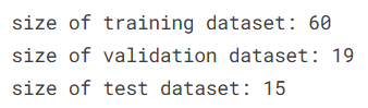
print(f"size of training dataset: {len(train_ds)}") # 训练集批次数
print(f"size of validation dataset: {len(val_ds)}") # 验证集批次数
print(f"size of test dataset: {len(test_ds)}") # 测试集批次数
4.2数据可视化

在模型训练前进行数据可视化分析非常重要。
通过可视化,我们可以:
-
检查类别分布是否均衡(是否存在类别不平衡问题)
-
直观查看图像样本质量
-
验证标签是否正确加载
-
初步理解数据结构
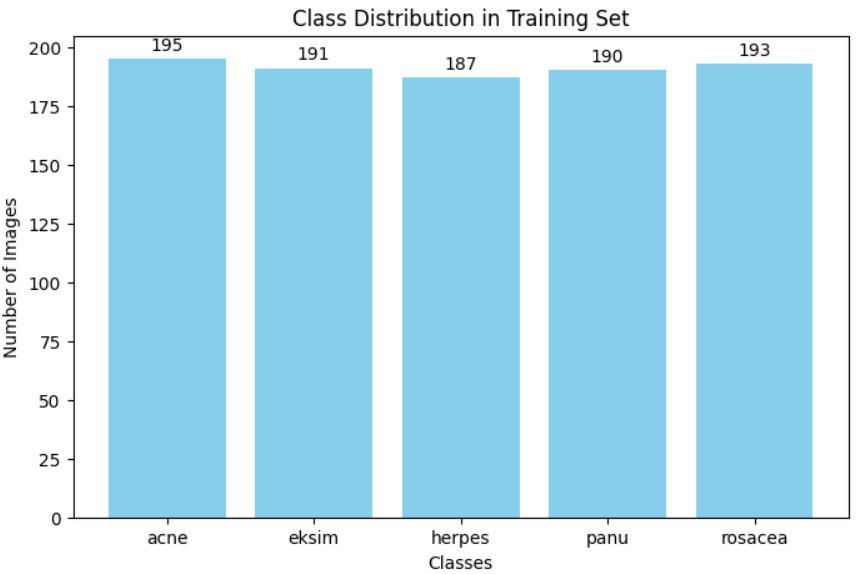
(1)类别分布可视化
本步骤统计训练集中各类别图像数量,并使用柱状图展示类别分布情况。这有助于判断数据是否存在类别不平衡问题(Class Imbalance)。
# ===============================
# 统计训练集中每个类别的样本数量
# ===============================

class_counts = Counter()  # 创建一个计数器对象,用于统计各类别数量

# 遍历训练数据集(按 batch 遍历)
for images, labels in train_ds:
    # labels.numpy() 将 Tensor 转换为 numpy 数组
    # update() 会自动统计每个类别出现的次数
    class_counts.update(labels.numpy())


# ===============================
# 绘制类别分布柱状图
# ===============================

plt.figure(figsize=(8,5))  # 设置图像尺寸

# 根据类别数量绘制柱状图
bars = plt.bar(
    class_names,                                 # x轴:类别名称
    [class_counts[i] for i in range(len(class_names))],  # y轴:对应类别数量
    color='skyblue'                              # 柱状图颜色
)

plt.title("Class Distribution in Training Set")  # 设置标题
plt.xlabel("Classes")                            # x轴标签
plt.ylabel("Number of Images")                   # y轴标签


# ===============================
# 在柱状图上方添加具体数量标签
# ===============================

for bar, count in zip(bars, [class_counts[i] for i in range(len(class_names))]):
    plt.text(
        bar.get_x() + bar.get_width()/2,   # x坐标:柱子中间
        bar.get_height() + 2,              # y坐标:柱子顶部稍微上方
        str(count),                        # 显示具体数值
        ha='center',                       # 水平居中
        va='bottom'                        # 垂直对齐方式
    )

plt.show()  # 显示图像
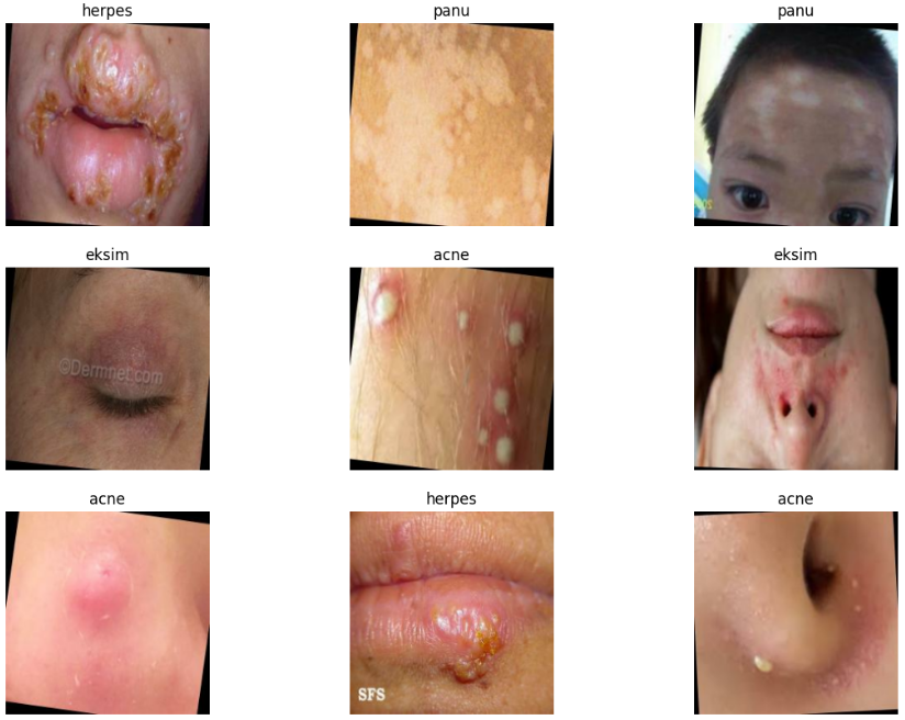
(2)训练样本可视化
本步骤随机展示训练集中一个 batch 的前 9 张图像,并标注其类别名称。
目的:
-
验证图像是否正确读取
-
检查图像尺寸是否正确缩放为 224×224
-
检查标签映射是否正确
# ===============================
# 可视化训练集中部分样本
# ===============================

plt.figure(figsize=(14,10))  # 设置画布大小

# 取训练集中的第一个 batch
for images, labels in train_ds.take(1):

    # 展示前 9 张图片
    for i in range(9):

        plt.subplot(3,3,i+1)  # 创建 3x3 子图布局

        # 将 Tensor 转换为 numpy 并转为 uint8 类型(便于显示)
        plt.imshow(images[i].numpy().astype('uint8'))

        # 显示类别名称
        plt.title(class_names[labels[i].numpy()])

        plt.axis('off')  # 关闭坐标轴


plt.show()  # 显示图像
4.3特征工程
在图像分类任务中,特征工程主要体现在两个方面:
-
迁移学习(Transfer Learning) —— 使用预训练模型提取高质量特征
-
数据增强(Data Augmentation) —— 提升模型泛化能力
-
数据管道优化(Pipeline Optimization) —— 提高训练效率
本实验基于 ImageNet 预训练的 ResNet50 进行迁移学习,并通过“部分冻结”策略进行微调(Fine-tuning),同时加入数据增强操作提升模型鲁棒性。
# ===============================
# 加载预训练 ResNet50 模型
# ===============================

base_model = ResNet50(
    include_top=False,         # 不包含原始全连接分类层(用于迁移学习)
    weights='imagenet',        # 加载 ImageNet 预训练权重
    input_shape=(224, 224, 3)  # 输入图像尺寸 (高, 宽, 通道数)
)


# ===============================
# 冻结前 140 层(迁移学习关键步骤)
# ===============================

# 冻结前 140 层参数(保留 ImageNet 学到的底层特征)
for layer in base_model.layers[:140]:
    layer.trainable = False   # 不参与反向传播更新

# 解冻后面层参数(用于微调)
for layer in base_model.layers[140:]:
    layer.trainable = True    # 参与训练更新
# ===============================
# 数据增强模块
# ===============================

data_augmentation = tf.keras.Sequential([
    layers.RandomFlip("horizontal"),  # 随机水平翻转
    layers.RandomRotation(0.1),       # 随机旋转 ±10%
    layers.RandomZoom(0.1),           # 随机缩放 ±10%
])
# ===============================
# 将数据增强应用到训练数据
# ===============================

train_ds = train_ds.map(
    lambda x, y: (data_augmentation(x, training=True), y)
)
# ===============================
# 提升数据加载性能
# ===============================

train_ds = train_ds.cache().prefetch(buffer_size=tf.data.AUTOTUNE)
val_ds = val_ds.cache().prefetch(buffer_size=tf.data.AUTOTUNE)
# ===============================
# ResNet50 专用归一化层
# ===============================

normalization = layers.Lambda(preprocess_input)
4.4构建模型
本部分基于迁移学习思想构建完整分类模型。模型整体结构为:
-
输入预处理层(ResNet50 专用归一化)
-
预训练 ResNet50 特征提取器
-
全局平均池化层(降维)
-
多层全连接网络(增强非线性表达能力)
-
Dropout 正则化(抑制过拟合)
-
Softmax 输出层(多分类任务)
同时设置:
-
Adam 优化器
-
早停机制(EarlyStopping)
-
学习率自适应衰减(ReduceLROnPlateau)
# ===============================
# 构建完整分类模型
# ===============================

model = Sequential([
    normalization,                # ResNet50 专用预处理层(对输入做归一化处理)
    base_model,                   # 预训练 ResNet50 特征提取网络

    layers.GlobalAveragePooling2D(),  # 全局平均池化层,将特征图转为一维向量
                                     # 相比 Flatten 可减少参数量,降低过拟合风险

    # ===============================
    # 全连接层(增强非线性表达能力)
    # ===============================

    layers.Dense(64, activation='relu'),   # 第一层全连接层
    layers.Dropout(0.3),                   # Dropout 正则化,随机丢弃 30% 神经元

    layers.Dense(128, activation='relu'),  # 第二层全连接层
    layers.Dropout(0.4),                   # 丢弃 40%

    layers.Dense(256, activation='relu'),  # 第三层全连接层
    layers.Dropout(0.4),                   # 丢弃 40%

    layers.Dense(128, activation='relu'),  # 新增一层全连接层(提升特征表达能力)
    layers.Dropout(0.3),                   # 丢弃 30%

    # ===============================
    # 输出层
    # ===============================

    layers.Dense(len(class_names), activation='softmax')
    # 输出节点数 = 类别数量
    # softmax 用于多分类问题,输出各类别概率
])


# ===============================
# 编译模型
# ===============================

model.compile(
    optimizer=tf.keras.optimizers.Adam(learning_rate=1e-3),
    # 使用 Adam 优化器
    # 学习率设置为 0.001(较常用初始学习率)

    loss='sparse_categorical_crossentropy',
    # 多分类损失函数(标签为整数编码时使用)

    metrics=['accuracy']
    # 评估指标:分类准确率
)


# ===============================
# 早停机制(防止过拟合)
# ===============================

early_stop = tf.keras.callbacks.EarlyStopping(
    monitor='val_loss',          # 监控验证集损失
    patience=5,                  # 若连续 5 个 epoch 无提升则停止训练
    restore_best_weights=True    # 恢复到验证集表现最好的权重
)


# ===============================
# 学习率动态衰减
# ===============================

lr_scheduler = tf.keras.callbacks.ReduceLROnPlateau(
    monitor='val_loss',   # 监控验证损失
    factor=0.3,           # 学习率缩小为原来的 0.3 倍
    patience=3,           # 3 个 epoch 无提升则调整学习率
    min_lr=1e-6,          # 最小学习率
    verbose=1             # 输出调整日志
)
技术要点说明
1️⃣ GlobalAveragePooling2D 优势
-
大幅减少参数量
-
避免过多全连接参数导致过拟合
-
在迁移学习中非常常见
2️⃣ 为什么使用多层 Dense + Dropout?
医学图像分类通常存在:
-
类别间细微差异
-
数据量相对有限
增加全连接层可以:
-
提升非线性建模能力
-
提取更高阶组合特征
增加 Dropout 可以:
-
抑制过拟合
-
提升泛化能力
3️⃣ EarlyStopping + ReduceLROnPlateau 的组合优势
这是工业级训练中非常常见的组合:
-
EarlyStopping:避免无效训练
-
ReduceLROnPlateau:在训练进入平台期时降低学习率
-
两者结合可以显著提升模型收敛效果
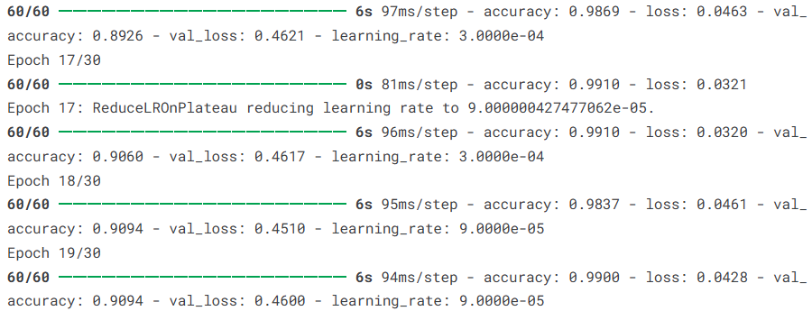
4.5训练模型
在训练过程中,模型会通过反向传播不断更新可训练参数,使损失函数最小化。
本实验设置:
-
最大训练轮数(epochs)为 30
-
使用验证集监控模型泛化能力
-
引入 EarlyStopping 防止过拟合
-
引入 ReduceLROnPlateau 动态调整学习率
# ===============================
# 开始模型训练
# ===============================

history = model.fit(
    train_ds,                 # 训练数据集(tf.data.Dataset 格式)
    epochs=30,                # 最大训练轮数(最多训练 30 个 epoch)
    validation_data=val_ds,   # 验证数据集,用于监控模型泛化能力
    callbacks=[early_stop, lr_scheduler]
    # 回调函数列表:
    # early_stop —— 验证损失不下降时提前停止训练
    # lr_scheduler —— 验证损失进入平台期时降低学习率
)
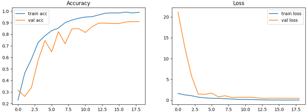
4.6模型评估
本节从多个维度对模型进行系统评估,包括:
-
训练过程可视化(Accuracy / Loss 曲线)
-
测试集整体性能评估
-
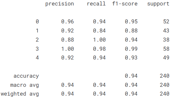
分类报告(Precision / Recall / F1-score)
-
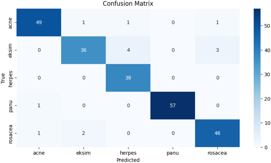
混淆矩阵分析
-
单样本预测可视化
通过这些指标,可以全面衡量模型的拟合情况与泛化能力。
# ===============================
# 1. 训练过程可视化(Accuracy & Loss 曲线)
# ===============================

plt.figure(figsize=(12,4))  # 设置整体画布大小

# ---- 准确率曲线 ----
plt.subplot(1,2,1)  # 1行2列,第1个子图
plt.plot(history.history['accuracy'], label='train acc')       # 训练准确率
plt.plot(history.history['val_accuracy'], label='val acc')     # 验证准确率
plt.title('Accuracy')                                           # 图标题
plt.legend()                                                    # 显示图例

# ---- 损失函数曲线 ----
plt.subplot(1,2,2)  # 第2个子图
plt.plot(history.history['loss'], label='train loss')           # 训练损失
plt.plot(history.history['val_loss'], label='val loss')         # 验证损失
plt.title('Loss')
plt.legend()

plt.show()
# ===============================
# 2. 测试集整体性能评估
# ===============================

# 为测试集添加缓存与预加载机制,提高推理效率
test_ds = test_ds.cache().prefetch(tf.data.AUTOTUNE)

# 在测试集上评估模型性能
test_loss, test_acc = model.evaluate(test_ds)

print("Test accuracy:", test_acc)  # 输出测试集准确率

# ===============================
# 3. 分类报告与混淆矩阵
# ===============================

y_true = []  # 存储真实标签
y_pred = []  # 存储预测标签

# 遍历测试数据集
for images, labels in test_ds:

    predictions = model.predict(images, verbose=0)
    # 得到每个类别的预测概率

    predicted = np.argmax(predictions, axis=1)
    # 取概率最大值对应的类别索引

    y_true.extend(labels.numpy())   # 真实标签
    y_pred.extend(predicted)        # 预测标签


# 生成分类报告(Precision / Recall / F1-score)
cm = classification_report(y_true, y_pred)
print(cm)

# 生成混淆矩阵
cm_matrix = confusion_matrix(y_true, y_pred)


# 可视化混淆矩阵
plt.figure(figsize=(10,5))
sns.heatmap(cm_matrix, annot=True, fmt='d', cmap='Blues',
            xticklabels=class_names, yticklabels=class_names)
plt.xlabel('Predicted')
plt.ylabel('True')
plt.title('Confusion Matrix')
plt.show()
# ===============================
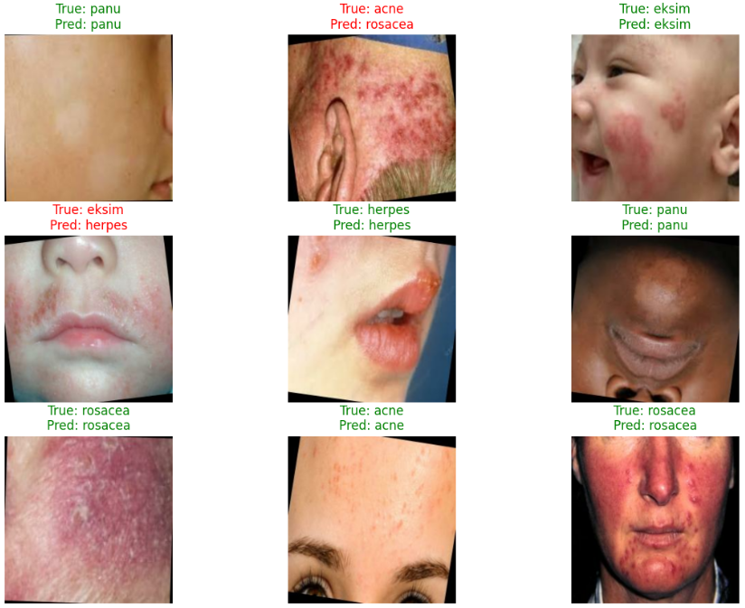
# 4. 测试样本预测可视化
# ===============================
plt.figure(figsize=(14, 10))
# 取测试集中的一个 batch
for images, labels in test_ds.take(1):
predictions = model.predict(images, verbose=0)
predicted_labels = np.argmax(predictions, axis=1)
for i in range(9): # 显示前 9 张图片
plt.subplot(3, 3, i+1)
plt.imshow(images[i].numpy().astype('uint8'))
true_label = class_names[labels[i].numpy()] # 真实标签
pred_label = class_names[predicted_labels[i]] # 预测标签
# 预测正确显示绿色,错误显示红色
color = 'green' if predicted_labels[i] == labels[i].numpy() else 'red'
plt.title(f"True: {true_label}\nPred: {pred_label}", color=color)
plt.axis('off')
5.总结
本实验基于 Kaggle 皮肤病图像数据集,构建了一个基于 ResNet50 迁移学习的皮肤疾病分类模型,实现了对痤疮(Acne)、湿疹(Eksim)、疱疹(Herpes)、潘努病(Panu)和酒渣鼻(Rosacea)五类皮肤疾病的自动识别。通过加载 ImageNet 预训练权重并采用部分冻结层的微调策略,在有限数据规模下有效提升了特征提取能力;同时结合数据增强、Dropout 正则化、EarlyStopping 以及学习率自适应调整等策略,有效抑制了过拟合并提升了模型的泛化性能。最终模型在测试集上取得了 94.17% 的准确率,macro avg 与 weighted avg 的 precision、recall 和 F1-score 均达到 0.94,整体分类表现稳定,其中对第3类疾病的识别效果尤为突出,而个别类别在召回率上仍存在一定提升空间。从整体实验结果来看,迁移学习在医学图像分类任务中具有较强的适用性和实用价值,本项目完整实现了从数据处理、特征工程、模型构建到性能评估的全流程,为后续进一步优化模型结构或扩展至更复杂医学影像场景奠定了实践基础。
# Standard Libraries
import os
import numpy as np
import seaborn as sns
import matplotlib.pyplot as plt
from collections import Counter

# Kaggle dataset helper
import kagglehub

# TensorFlow / Keras
import tensorflow as tf
from tensorflow.keras import layers
from tensorflow.keras.models import Sequential
from tensorflow.keras.preprocessing import image_dataset_from_directory
from tensorflow.keras.applications.resnet50 import ResNet50
from tensorflow.keras.applications.resnet50 import preprocess_input

# Metrics
from sklearn.metrics import classification_report
from sklearn.metrics import confusion_matrix

# Ignore warnings
import warnings
warnings.filterwarnings("ignore")
# Suppress TensorFlow logs
os.environ['TF_CPP_MIN_LOG_LEVEL'] = '3'
import tensorflow as tf
path = kagglehub.dataset_download("sponishflea/classification-of-skin-diseases")
# Training directory
data_dir=os.path.join(path,'train')

# Image settings
image_size=(224,224)
batch_size=16
# Split into training and validation
train_ds=image_dataset_from_directory(
    data_dir,
    image_size=image_size,
    batch_size=batch_size,
    subset='training',
    validation_split=0.2,
    seed=46,
    label_mode='int'
)
val_ds=image_dataset_from_directory(
    data_dir,
    image_size=image_size,
    batch_size=batch_size,
    subset='validation',
    validation_split=0.2,
    seed=46,
    label_mode='int'
)
class_names=train_ds.class_names
test_size=int(len(train_ds)*0.2)

test_ds=train_ds.take(test_size)
train_ds=train_ds.skip(test_size)
print(f"size of training dataset: { len(train_ds)}")
print(f"size of validation dataset: { len(val_ds)}")
print(f"size of test dataset: { len(test_ds)}")
class_counts = Counter()
for images, labels in train_ds:
    class_counts.update(labels.numpy())
plt.figure(figsize=(8,5))
bars = plt.bar(class_names, [class_counts[i] for i in range(len(class_names))], color='skyblue')
plt.title("Class Distribution in Training Set")
plt.xlabel("Classes")
plt.ylabel("Number of Images")

# Add counts on top of bars
for bar, count in zip(bars, [class_counts[i] for i in range(len(class_names))]):
    plt.text(bar.get_x() + bar.get_width()/2, bar.get_height() + 2, str(count), ha='center', va='bottom')

plt.show()
plt.figure(figsize=(14,10))

for images, labels in train_ds.take(1):
    for i in range(9):
        plt.subplot(3,3,i+1)
        plt.imshow(images[i].numpy().astype('uint8'))
        plt.title(class_names[labels[i].numpy()])
        plt.axis('off')

plt.show()
base_model = ResNet50(
    include_top=False,
    weights='imagenet',
    input_shape=(224, 224, 3)
)

for layer in base_model.layers[:140]:
    layer.trainable = False
for layer in base_model.layers[140:]:
    layer.trainable = True

data_augmentation = tf.keras.Sequential([
    layers.RandomFlip("horizontal"),
    layers.RandomRotation(0.1),
    layers.RandomZoom(0.1),
])

train_ds = train_ds.map(
    lambda x, y: (data_augmentation(x, training=True), y)
)
train_ds = train_ds.cache().prefetch(buffer_size=tf.data.AUTOTUNE)
val_ds = val_ds.cache().prefetch(buffer_size=tf.data.AUTOTUNE)
normalization = layers.Lambda(preprocess_input)
model = Sequential([
    normalization,
    base_model,
    layers.GlobalAveragePooling2D(),

    # Fully connected layers with more Dropout
    layers.Dense(64, activation='relu'),
    layers.Dropout(0.3),      # increased dropout

    layers.Dense(128, activation='relu'),
    layers.Dropout(0.4),

    layers.Dense(256, activation='relu'),
    layers.Dropout(0.4),

    layers.Dense(128, activation='relu'),  # added one more layer
    layers.Dropout(0.3),

    layers.Dense(len(class_names), activation='softmax')
])

model.compile(
    optimizer=tf.keras.optimizers.Adam(learning_rate=1e-3),
    loss='sparse_categorical_crossentropy',
    metrics=['accuracy']
)
early_stop = tf.keras.callbacks.EarlyStopping(
    monitor='val_loss',
    patience=5,
    restore_best_weights=True
)

lr_scheduler = tf.keras.callbacks.ReduceLROnPlateau(
    monitor='val_loss',
    factor=0.3,
    patience=3,
    min_lr=1e-6,
    verbose=1
)
history = model.fit(
    train_ds,
    epochs=30,
    validation_data=val_ds,
    callbacks=[early_stop, lr_scheduler]
)
plt.figure(figsize=(12,4))

plt.subplot(1,2,1)
plt.plot(history.history['accuracy'], label='train acc')
plt.plot(history.history['val_accuracy'], label='val acc')
plt.title('Accuracy')
plt.legend()

plt.subplot(1,2,2)
plt.plot(history.history['loss'], label='train loss')
plt.plot(history.history['val_loss'], label='val loss')
plt.title('Loss')
plt.legend()

plt.show()
test_ds = test_ds.cache().prefetch(tf.data.AUTOTUNE)

test_loss, test_acc = model.evaluate(test_ds)
print("Test accuracy:", test_acc)
y_true = []
y_pred = []

for images, labels in test_ds:
    predictions = model.predict(images,verbose=0)
    predicted = np.argmax(predictions, axis=1)

    y_true.extend(labels.numpy())
    y_pred.extend(predicted)

cm=classification_report(y_true,y_pred)
print(cm)
cm_matrix = confusion_matrix(y_true, y_pred)

plt.figure(figsize=(10,5))
sns.heatmap(cm_matrix, annot=True, fmt='d', cmap='Blues',
            xticklabels=class_names, yticklabels=class_names)
plt.xlabel('Predicted')
plt.ylabel('True')
plt.title('Confusion Matrix')
plt.show()
plt.figure(figsize=(14, 10))
for images, labels in test_ds.take(1):
    predictions = model.predict(images, verbose=0)
    predicted_labels = np.argmax(predictions, axis=1)

    for i in range(9):  # Display first 9 images
        plt.subplot(3, 3, i+1)
        plt.imshow(images[i].numpy().astype('uint8'))

        true_label = class_names[labels[i].numpy()]
        pred_label = class_names[predicted_labels[i]]

        color = 'green' if predicted_labels[i] == labels[i].numpy() else 'red'
        plt.title(f"True: {true_label}\nPred: {pred_label}", color=color)

        plt.axis('off')
plt.show()
资料获取,更多粉丝福利,关注下方公众号获取


AtomGit 是由开放原子开源基金会联合 CSDN 等生态伙伴共同推出的新一代开源与人工智能协作平台。平台坚持“开放、中立、公益”的理念,把代码托管、模型共享、数据集托管、智能体开发体验和算力服务整合在一起,为开发者提供从开发、训练到部署的一站式体验。
更多推荐


 22
22 0
0- 0


 已为社区贡献6条内容

所有评论(0)