【雷达信号优化】第一章雷达信号模型与数学基础

VectorShift

353人浏览 · 2026-03-29 19:03:09

VectorShift · 2026-03-29 19:03:09 发布

1.1.2.1.1 Swerling目标起伏模型

1.1.2.1.2 Neyman-Pearson准则

1.2.2.1.1 调频斜率对脉冲压缩的影响

第一章雷达信号模型与数学基础

1.1 雷达方程与信噪比优化

雷达系统设计的核心在于建立电磁能量传播的数学模型，通过优化理论在约束条件下最大化系统性能指标。本章从经典雷达方程出发，构建信号处理的数学框架，明确优化问题的定义域与约束条件。

1.1.1 经典雷达方程推导

雷达方程描述了发射功率、天线增益、目标截面积、传播损耗与接收信噪比之间的定量关系。基于电磁波传播理论，接收功率 Pr 可表示为：

自由空间路径损耗随频率和距离变化

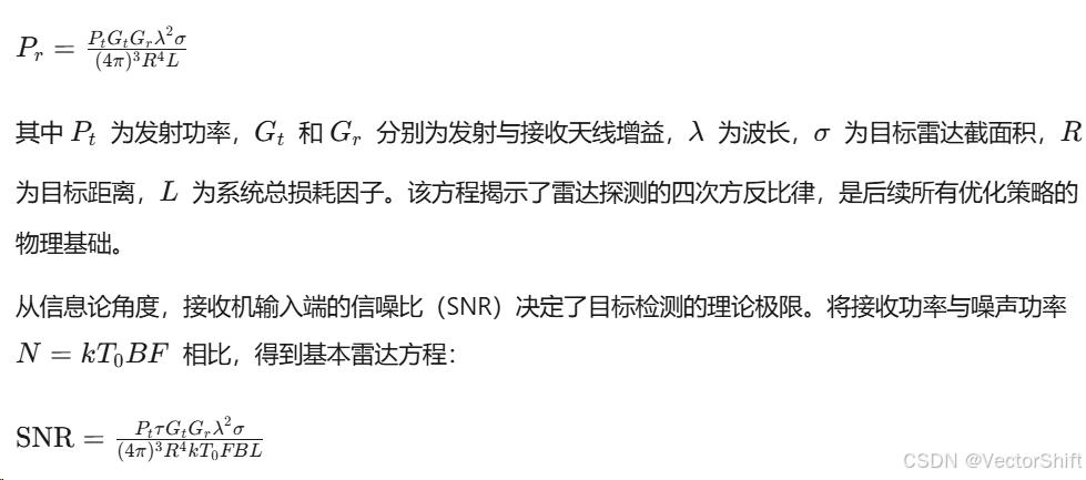
1.1.1.1 射频损耗模型

实际雷达系统中，射频链路存在多种非理想因素导致能量衰减。损耗模型需精确量化各环节对信噪比的影响，为系统优化提供约束条件。总损耗 L 通常分解为：

$L = L_{\text{atm}} \cdot L_{\text{sys}} \cdot L_{\text{pol}} \cdot L_{\text{mism}}$

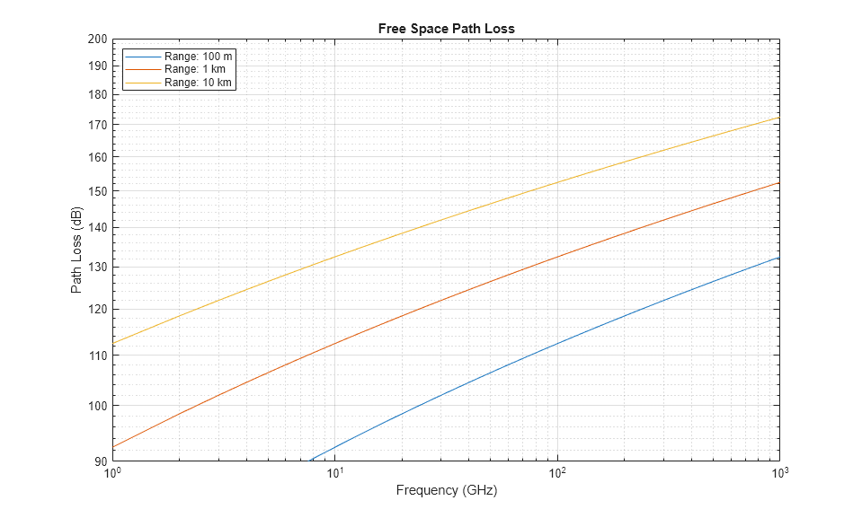
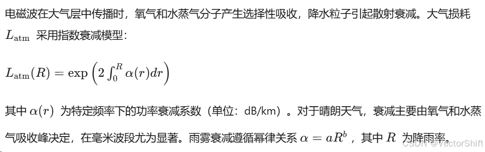
1.1.1.1.1 大气传播损耗

%% 脚本：Atmospheric_Loss_Model.m
% 内容：大气传播损耗建模与频率/距离特性分析
% 使用方式：直接运行，生成大气衰减系数随频率变化曲线及不同天气条件下的路径损耗
% 优化要点：采用ITU-R模型计算氧气/水蒸气吸收，支持多频段雷达系统设计

clear; clc; close all;

% 参数设置
freq = linspace(1, 100, 500); % 频率范围 1-100 GHz
distance = [1, 5, 10, 50, 100]; % 距离 (km)
% 环境参数
T = 288.15; % 温度 (K)
P = 1013.25; % 气压 (hPa)
rho = 7.5; % 水蒸气密度 (g/m^3)

% 计算氧气和水蒸气衰减系数 (ITU-R P.676模型简化)
% 氧气吸收线：50-70 GHz band, 118.75 GHz等
% 水蒸气吸收线：22.3 GHz, 183.31 GHz等
gamma_o = zeros(size(freq)); % 氧气衰减
gamma_w = zeros(size(freq)); % 水蒸气衰减

for i = 1:length(freq)
    f = freq(i);
    % 氧气衰减系数 (dB/km) - 简化模型
    gamma_o(i) = (7.2e-3 + 6.5e-5*f + 3.2e-7*f.^2) .* exp(-f/50);
    
    % 水蒸气衰减系数 (dB/km)
    if f < 350
        gamma_w(i) = 0.05 * (rho/7.5) * (f/22.3).^2 .* exp(-((f-22.3)/20).^2) + ...
                     0.001 * (f/100).^2.5;
    else
        gamma_w(i) = 0.01 * (f/100).^2;
    end
end

gamma_total = gamma_o + gamma_w; % 总衰减系数 (dB/km)

% 可视化 1: 衰减系数随频率变化
figure('Position', [100, 100, 800, 600], 'Color', 'w');
semilogy(freq, gamma_o, 'b-', 'LineWidth', 2); hold on;
semilogy(freq, gamma_w, 'r--', 'LineWidth', 2);
semilogy(freq, gamma_total, 'k-', 'LineWidth', 2.5);
xlabel('Frequency (GHz)', 'FontSize', 12, 'FontWeight', 'bold');
ylabel('Attenuation Coefficient (dB/km)', 'FontSize', 12, 'FontWeight', 'bold');
title('Atmospheric Attenuation vs Frequency (Clear Air)', 'FontSize', 14, 'FontWeight', 'bold');
legend('Oxygen', 'Water Vapor', 'Total', 'Location', 'northwest');
grid on; axis tight;
set(gca, 'FontSize', 11);

% 可视化 2: 不同距离下的累积路径损耗
figure('Position', [150, 150, 800, 600], 'Color', 'w');
colors = jet(length(distance));
for i = 1:length(distance)
    d = distance(i);
    path_loss = gamma_total * d; % 单程损耗 (dB)
    plot(freq, path_loss, 'Color', colors(i,:), 'LineWidth', 2, ...
         'DisplayName', sprintf('%.0f km', d)); hold on;
end
xlabel('Frequency (GHz)', 'FontSize', 12, 'FontWeight', 'bold');
ylabel('Total Path Loss (dB)', 'FontSize', 12, 'FontWeight', 'bold');
title('Atmospheric Path Loss for Various Ranges', 'FontSize', 14, 'FontWeight', 'bold');
legend('show', 'Location', 'northwest');
grid on; axis tight;
set(gca, 'FontSize', 11);

% 可视化 3: 雨雾衰减模型 (Marshall-Palmer分布)
rain_rate = [0, 1, 4, 16, 50]; % mm/h: 晴, 小雨, 中雨, 大雨, 暴雨
figure('Position', [200, 200, 800, 600], 'Color', 'w');
freq_rain = linspace(1, 50, 200);
for i = 1:length(rain_rate)
    R = rain_rate(i);
    % 简化雨衰减模型: alpha = a * R^b (dB/km)
    a = 0.0001 * freq_rain.^2; % 频率依赖系数
    b = 1.2; % 降雨率指数
    alpha_rain = a .* R.^b;
    plot(freq_rain, alpha_rain, 'LineWidth', 2, ...
         'DisplayName', sprintf('Rain: %.0f mm/h', R)); hold on;
end
xlabel('Frequency (GHz)', 'FontSize', 12, 'FontWeight', 'bold');
ylabel('Specific Attenuation (dB/km)', 'FontSize', 12, 'FontWeight', 'bold');
title('Rain Attenuation vs Frequency', 'FontSize', 14, 'FontWeight', 'bold');
legend('show', 'Location', 'northwest');
grid on; set(gca, 'FontSize', 11);

% 优化建议输出
fprintf('=== 大气损耗分析完成 ===\n');
fprintf('关键频段损耗参考 (10km路径):\n');
idx_10GHz = find(freq >= 10, 1);
idx_35GHz = find(freq >= 35, 1);
idx_94GHz = find(freq >= 94, 1);
fprintf('  X-band (10 GHz): %.2f dB\n', gamma_total(idx_10GHz)*10);
fprintf('  Ka-band (35 GHz): %.2f dB\n', gamma_total(idx_35GHz)*10);
fprintf('  W-band (94 GHz): %.2f dB\n', gamma_total(idx_94GHz)*10);

1.1.1.1.2 系统噪声系数

接收机内部噪声由有源器件的热噪声和散粒噪声主导。噪声系数 F 量化接收机相对于理想系统的信噪比退化程度，定义为输入信噪比与输出信噪比之比：

$F = \frac{\text{SNR}_{\text{in}}}{\text{SNR}_{\text{out}}} = 1 + \frac{T_e}{T_0}$

其中 $T_e$ 为等效噪声温度。对于多级级联系统，Friis公式给出总噪声系数：

$F_{\text{total}} = F_1 + \frac{F_2-1}{G_1} + \frac{F_3-1}{G_1 G_2} + \cdots$

该表达式揭示第一级低噪声放大器（LNA）的噪声系数和增益对系统性能的决定性作用，为硬件优化提供明确方向：优先优化前端噪声性能。

%% 脚本：Noise_Figure_Analysis.m
% 内容：级联系统噪声系数计算与灵敏度分析
% 使用方式：定义各级器件参数，计算总噪声系数和等效噪声温度
% 优化要点：支持任意级数级联，自动识别关键噪声贡献级

clear; clc; close all;

% 典型雷达接收机链路参数
% 格式: [噪声系数(dB), 增益(dB), 名称]
stages = {
    2.5, 20, 'LNA';           % 低噪声放大器
    1.0, -3, 'Filter';        % 带通滤波器
    10.0, 30, 'Mixer';        % 混频器
    15.0, 25, 'IF_Amp';       % 中频放大器
    8.0, 0, 'Detector';       % 检波器
    12.0, 40, 'Video_Amp'     % 视频放大器
};

num_stages = size(stages, 1);
F = zeros(num_stages, 1); % 线性噪声系数
G = zeros(num_stages, 1); % 线性增益
labels = cell(num_stages, 1);

for i = 1:num_stages
    F(i) = 10^(stages{i,1}/10); % dB to linear
    G(i) = 10^(stages{i,2}/10); % dB to linear
    labels{i} = stages{i,3};
end

% 级联噪声系数计算 (Friis公式)
F_cascade = zeros(num_stages, 1);
G_product = 1;
F_cumulative = 0;

for i = 1:num_stages
    if i == 1
        F_cumulative = F(i);
        G_product = G(i);
    else
        F_cumulative = F_cumulative + (F(i)-1)/G_product;
        G_product = G_product * G(i);
    end
    F_cascade(i) = 10*log10(F_cumulative); % dB
end

F_total_dB = 10*log10(F_cumulative);
T0 = 290; % 标准温度 (K)
Te = (F_cumulative - 1) * T0; % 等效噪声温度

% 灵敏度计算
k = 1.38e-23; % 玻尔兹曼常数
B = 1e6; % 带宽 1 MHz
SNR_req = 13; % 所需信噪比 (dB)
Noise_Floor = 10*log10(k*T0*B) + F_total_dB; % dBm
Sensitivity = Noise_Floor + SNR_req; % dBm

% 可视化 1: 级联噪声系数贡献
figure('Position', [100, 100, 900, 600], 'Color', 'w');
bar(F_cascade, 'FaceColor', [0.2 0.4 0.8]);
set(gca, 'XTickLabel', labels, 'FontSize', 11);
xlabel('Stage Index', 'FontSize', 12, 'FontWeight', 'bold');
ylabel('Cumulative Noise Figure (dB)', 'FontSize', 12, 'FontWeight', 'bold');
title(sprintf('Cascaded Noise Figure Analysis (Total: %.2f dB)', F_total_dB), ...
      'FontSize', 14, 'FontWeight', 'bold');
grid on; ylim([0, max(F_cascade)*1.2]);
for i = 1:num_stages
    text(i, F_cascade(i)+0.3, sprintf('%.2f', F_cascade(i)), ...
         'HorizontalAlignment', 'center', 'FontWeight', 'bold');
end

% 可视化 2: 各级贡献分解 (饼图)
figure('Position', [150, 150, 800, 600], 'Color', 'w');
contributions = zeros(num_stages, 1);
contrib_product = 1;
for i = 1:num_stages
    if i == 1
        contributions(i) = F(i) - 1;
        contrib_product = G(i);
    else
        contributions(i) = (F(i)-1)/contrib_product;
        contrib_product = contrib_product * G(i);
    end
end
contributions = contributions / sum(contributions) * 100; % 百分比

pie(contributions, labels);
title('Noise Contribution by Stage (Relative Impact)', 'FontSize', 14, 'FontWeight', 'bold');
colormap(jet(num_stages));

% 可视化 3: 增益 vs 噪声系数权衡分析
figure('Position', [200, 200, 900, 600], 'Color', 'w');
% 参数扫描: LNA噪声系数和增益变化
lna_nf_range = 0.5:0.1:5; % dB
lna_gain_range = 10:2:30; % dB

[X, Y] = meshgrid(lna_nf_range, lna_gain_range);
Z = zeros(size(X));

for i = 1:size(X,1)
    for j = 1:size(X,2)
        F_lna = 10^(X(i,j)/10);
        G_lna = 10^(Y(i,j)/10);
        % 其余级固定
        F_rest = F(2);
        G_rest = prod(G(2:end-1));
        F_sys = F_lna + (F_rest-1)/G_lna;
        Z(i,j) = 10*log10(F_sys);
    end
end

surf(X, Y, Z, 'EdgeColor', 'none');
xlabel('LNA Noise Figure (dB)', 'FontSize', 12, 'FontWeight', 'bold');
ylabel('LNA Gain (dB)', 'FontSize', 12, 'FontWeight', 'bold');
zlabel('Total System NF (dB)', 'FontSize', 12, 'FontWeight', 'bold');
title('LNA Parameter Trade-off Analysis', 'FontSize', 14, 'FontWeight', 'bold');
colorbar; shading interp; view(45, 30);
grid on;

% 结果输出
fprintf('=== 接收机噪声分析结果 ===\n');
fprintf('总噪声系数: %.2f dB\n', F_total_dB);
fprintf('等效噪声温度: %.2f K\n', Te);
fprintf('接收机灵敏度 (SNR=%ddB): %.2f dBm\n', SNR_req, Sensitivity);
fprintf('关键噪声贡献级: %s (%.1f%%)\n', labels{1}, contributions(1));

1.1.2 信噪比作为核心优化目标

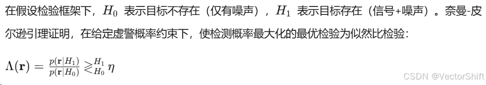
雷达检测本质上是二元假设检验问题。在噪声背景下判断目标存在与否，需要优化检测概率 $P_d$ 与虚警概率 $P_{fa}$ 之间的权衡关系。奈曼-皮尔逊准则在此框架下确立了似然比检验的最优性，而信噪比作为充分统计量直接决定检测性能边界。

对于平方律检波器，检测概率与虚警概率通过Marcum Q函数关联：

$P_d = Q_M\left(\sqrt{2\text{SNR}}, \sqrt{-2\ln P_{fa}}\right)$

其中 $Q_M$ 为广义Marcum Q函数。该关系式明确表明，在给定虚警概率约束下，最大化检测概率等价于最大化信噪比，确立了SNR作为雷达信号处理核心优化指标的理论地位。

1.1.2.1 检测概率与虚警概率

1.1.2.1.1 Swerling目标起伏模型

实际雷达目标由多个散射中心组成，其回波幅度随视角变化产生起伏。Swerling模型基于散射中心统计特性将目标分为四类：

Swerling I/II：慢起伏（扫描间相关），瑞利分布包络，χ2 分布2自由度
Swerling III/IV：快起伏（脉冲间独立），包络分布含主导散射体

检测概率计算需对目标起伏进行统计平均。对于Swerling I型目标，检测概率为：

$P_d = \left[P_{fa}\right]^{\frac{1}{1+\text{SNR}}}$

该表达式表明起伏目标需要更高的平均信噪比才能达到与稳定目标相同的检测性能，通常需要增加5-10 dB的信噪比裕度。

%% 脚本：Swerling_Model_Detection.m
% 内容：Swerling起伏目标检测概率计算与性能分析
% 使用方式：设置虚警概率和SNR范围，计算四种Swerling模型的检测性能
% 优化要点：包含非相干积累增益，支持脉冲数优化分析

clear; clc; close all;

% 参数设置
Pfa = 1e-6; % 虚警概率
SNR_dB = linspace(0, 30, 200); % 信噪比范围 (dB)
SNR = 10.^(SNR_dB/10); % 线性信噪比
N_pulses = [1, 10, 50, 100]; % 非相干积累脉冲数

% 计算检测概率函数
Pd_SW1 = @(snr, n) (Pfa.^(1./(1+snr))).^n; % Swerling I (近似多脉冲)
Pd_SW2 = @(snr, n) 1 - (1-Pfa).^(1./(1+snr)); % Swerling II (独立脉冲)
Pd_SW3 = @(snr, n) (1 + 2*snr./(2+snr*n)).^2 .* Pfa.^((1+snr)./(1+2*snr)); % Swerling III
Pd_SW4 = @(snr, n) 1 - (1-Pfa).^((1+snr).^2./(1+2*snr)); % Swerling IV

% Marcum Q函数近似 (稳定目标)
Pd_marcum = @(snr, n) marcumq(sqrt(2*snr*n), sqrt(-2*log(Pfa)));

% 可视化 1: 单脉冲检测性能对比
figure('Position', [100, 100, 900, 600], 'Color', 'w');
Pd_SNR_SW1 = Pd_SW1(SNR, 1);
Pd_SNR_SW2 = Pd_SW2(SNR, 1);
Pd_SNR_SW3 = Pd_SW3(SNR, 1);
Pd_SNR_SW4 = Pd_SW4(SNR, 1);

plot(SNR_dB, Pd_SNR_SW1, 'b-', 'LineWidth', 2); hold on;
plot(SNR_dB, Pd_SNR_SW2, 'r--', 'LineWidth', 2);
plot(SNR_dB, Pd_SNR_SW3, 'g-.', 'LineWidth', 2);
plot(SNR_dB, Pd_SNR_SW4, 'm:', 'LineWidth', 2);
plot(SNR_dB, Pd_marcum(SNR, 1), 'k-', 'LineWidth', 2.5);

xlabel('Single-Pulse SNR (dB)', 'FontSize', 12, 'FontWeight', 'bold');
ylabel('Probability of Detection', 'FontSize', 12, 'FontWeight', 'bold');
title('Detection Performance: Swerling Target Models (P_{fa}=10^{-6})', ...
      'FontSize', 14, 'FontWeight', 'bold');
legend('Swerling I', 'Swerling II', 'Swerling III', 'Swerling IV', ...
       'Non-fluctuating', 'Location', 'southeast');
grid on; ylim([0, 1]); set(gca, 'FontSize', 11);

% 可视化 2: 非相干积累对Swerling I的改善
figure('Position', [150, 150, 900, 600], 'Color', 'w');
colors = lines(length(N_pulses));
for i = 1:length(N_pulses)
    N = N_pulses(i);
    % 积累后等效SNR (近似)
    snr_eff = SNR * N; % 非相干积累增益约sqrt(N)
    Pd = Pd_SW1(snr_eff/N, N); % 修正模型
    plot(SNR_dB, Pd, 'Color', colors(i,:), 'LineWidth', 2, ...
         'DisplayName', sprintf('%d Pulses', N)); hold on;
end
xlabel('Single-Pulse SNR (dB)', 'FontSize', 12, 'FontWeight', 'bold');
ylabel('Probability of Detection', 'FontSize', 12, 'FontWeight', 'bold');
title('Non-coherent Integration: Swerling I Target', 'FontSize', 14, 'FontWeight', 'bold');
legend('show', 'Location', 'southeast');
grid on; ylim([0, 1]); set(gca, 'FontSize', 11);

% 可视化 3: 所需SNR vs 检测概率 (ROC曲线族)
figure('Position', [200, 200, 900, 600], 'Color', 'w');
Pd_target = 0.5:0.1:0.95;
SNR_req_SW1 = zeros(size(Pd_target));
SNR_req_SW2 = zeros(size(Pd_target));
SNR_req_SW3 = zeros(size(Pd_target));
SNR_req_SW4 = zeros(size(Pd_target));

for i = 1:length(Pd_target)
    pd = Pd_target(i);
    % 数值反解所需SNR
    SNR_req_SW1(i) = fzero(@(s) Pd_SW1(10^(s/10),1)-pd, 20);
    SNR_req_SW2(i) = fzero(@(s) Pd_SW2(10^(s/10),1)-pd, 20);
    SNR_req_SW3(i) = fzero(@(s) Pd_SW3(10^(s/10),1)-pd, 20);
    SNR_req_SW4(i) = fzero(@(s) Pd_SW4(10^(s/10),1)-pd, 20);
end

plot(Pd_target, SNR_req_SW1, 'b-o', 'LineWidth', 2); hold on;
plot(Pd_target, SNR_req_SW2, 'r-s', 'LineWidth', 2);
plot(Pd_target, SNR_req_SW3, 'g-^', 'LineWidth', 2);
plot(Pd_target, SNR_req_SW4, 'm-d', 'LineWidth', 2);
xlabel('Required Probability of Detection', 'FontSize', 12, 'FontWeight', 'bold');
ylabel('Required SNR (dB)', 'FontSize', 12, 'FontWeight', 'bold');
title('SNR Requirement vs Detection Probability (P_{fa}=10^{-6})', ...
      'FontSize', 14, 'FontWeight', 'bold');
legend('Swerling I', 'Swerling II', 'Swerling III', 'Swerling IV', ...
       'Location', 'northwest');
grid on; set(gca, 'FontSize', 11);

% 起伏损失计算
SNR_sw0 = fzero(@(s) Pd_marcum(10^(s/10),1)-0.9, 15); % 稳定目标
SNR_sw1 = fzero(@(s) Pd_SW1(10^(s/10),1)-0.9, 20);
fluctuation_loss = SNR_sw1 - SNR_sw0;

fprintf('=== Swerling模型分析结果 ===\n');
fprintf('达到Pd=0.9, Pfa=1e-6所需SNR:\n');
fprintf('  非起伏目标: %.1f dB\n', SNR_sw0);
fprintf('  Swerling I: %.1f dB\n', SNR_sw1);
fprintf('  起伏损失: %.1f dB\n', fluctuation_loss);

1.1.2.1.2 Neyman-Pearson准则

其中阈值 η 由虚警概率约束确定。对于高斯噪声中的确定性信号，该准则退化为匹配滤波器结构，输出信噪比最大化等价于似然比最大化。

接收机工作特性（ROC）曲线描绘了不同信噪比下检测概率与虚警概率的权衡关系，是评估检测系统性能的标准工具。

%% 脚本：Neyman_Pearson_Optimal_Detection.m
% 内容：奈曼-皮尔逊准则下的最优检测器实现与ROC分析
% 使用方式：生成信号+噪声样本，实现似然比检验，绘制ROC曲线
% 优化要点：包含匹配滤波器实现，展示充分统计量与SNR关系

clear; clc; close all;

% 参数设置
N_samples = 1000; % 信号样本数
SNR_dB = [-10, -5, 0, 5, 10]; % 不同信噪比 (dB)
N_trials = 10000; % 蒙特卡洛试验次数
signal = ones(N_samples, 1); % 确定性信号 (直流为例)
signal = signal / norm(signal); % 单位能量归一化

% 可视化 1: 匹配滤波器响应示例
figure('Position', [100, 100, 900, 600], 'Color', 'w');
snr_example = 0; % dB
noise_var = 10^(-snr_example/10);
noise = sqrt(noise_var) * randn(N_samples, 1);
received_H0 = noise;
received_H1 = signal + noise;

% 匹配滤波 (相关器)
mf_output_H0 = cumsum(received_H0 .* signal);
mf_output_H1 = cumsub= cumsum(received_H1 .* signal);

subplot(2,1,1);
plot(received_H0, 'b', 'LineWidth', 1); hold on;
plot(received_H1, 'r', 'LineWidth', 1.5);
plot(signal*max(abs(received_H0)), 'k--', 'LineWidth', 2);
title('Received Signal Waveforms', 'FontSize', 12, 'FontWeight', 'bold');
legend('Noise Only (H_0)', 'Signal+Noise (H_1)', 'Signal Template');
grid on;

subplot(2,1,2);
plot(mf_output_H0, 'b', 'LineWidth', 1.5); hold on;
plot(mf_output_H1, 'r', 'LineWidth', 1.5);
xlabel('Sample Index', 'FontSize', 11);
ylabel('Matched Filter Output', 'FontSize', 11);
title('Matched Filter Integration (Cumulative)', 'FontSize', 12, 'FontWeight', 'bold');
legend('H_0', 'H_1'); grid on;

% 可视化 2: ROC曲线生成
figure('Position', [150, 150, 900, 700], 'Color', 'w');
colors = jet(length(SNR_dB));

for idx = 1:length(SNR_dB)
    snr_db = SNR_dB(idx);
    snr_lin = 10^(snr_db/10);
    noise_var = 1/snr_lin; % 信号功率归一化为1
    
    % 生成检验统计量 (匹配滤波器输出)
    % H0: 纯噪声 ~ N(0, noise_var/N_samples) (积分后)
    % H1: 信号+噪声 ~ N(1, noise_var/N_samples)
    T_H0 = sqrt(noise_var) * randn(N_trials, 1) / sqrt(N_samples);
    T_H1 = 1 + sqrt(noise_var) * randn(N_trials, 1) / sqrt(N_samples);
    
    % 计算不同阈值下的Pd和Pfa
    thresholds = linspace(min(T_H0)-0.5, max(T_H1)+0.5, 200);
    Pfa = zeros(size(thresholds));
    Pd = zeros(size(thresholds));
    
    for i = 1:length(thresholds)
        eta = thresholds(i);
        Pfa(i) = mean(T_H0 > eta);
        Pd(i) = mean(T_H1 > eta);
    end
    
    % 绘制ROC
    semilogx(Pfa, Pd, 'Color', colors(idx,:), 'LineWidth', 2.5, ...
             'DisplayName', sprintf('SNR = %d dB', snr_db)); hold on;
end

xlabel('Probability of False Alarm (P_{fa})', 'FontSize', 12, 'FontWeight', 'bold');
ylabel('Probability of Detection (P_d)', 'FontSize', 12, 'FontWeight', 'bold');
title('ROC Curves: Neyman-Pearson Optimal Detector', 'FontSize', 14, 'FontWeight', 'bold');
legend('show', 'Location', 'southeast');
grid on; xlim([1e-6, 1]); ylim([0, 1]);
set(gca, 'FontSize', 11);

% 可视化 3: 检测统计量分布直方图
figure('Position', [200, 200, 900, 600], 'Color', 'w');
snr_plot = 5; % dB
snr_lin = 10^(snr_plot/10);
noise_var = 1/snr_lin;

T_H0_dist = sqrt(noise_var) * randn(50000, 1) / sqrt(N_samples);
T_H1_dist = 1 + sqrt(noise_var) * randn(50000, 1) / sqrt(N_samples);

histogram(T_H0_dist, 50, 'Normalization', 'pdf', 'FaceColor', 'b', ...
          'FaceAlpha', 0.5, 'EdgeColor', 'none'); hold on;
histogram(T_H1_dist, 50, 'Normalization', 'pdf', 'FaceColor', 'r', ...
          'FaceAlpha', 0.5, 'EdgeColor', 'none');

% 理论分布曲线
x_range = linspace(min(T_H0_dist), max(T_H1_dist), 200);
pdf_H0 = normpdf(x_range, 0, sqrt(noise_var/N_samples));
pdf_H1 = normpdf(x_range, 1, sqrt(noise_var/N_samples));
plot(x_range, pdf_H0, 'b-', 'LineWidth', 3);
plot(x_range, pdf_H1, 'r-', 'LineWidth', 3);

xlabel('Test Statistic', 'FontSize', 12, 'FontWeight', 'bold');
ylabel('Probability Density', 'FontSize', 12, 'FontWeight', 'bold');
title(sprintf('Likelihood Functions (SNR = %d dB)', snr_plot), ...
      'FontSize', 14, 'FontWeight', 'bold');
legend('H_0 Empirical', 'H_1 Empirical', 'H_0 Theory', 'H_1 Theory');
grid on; set(gca, 'FontSize', 11);

% 计算并显示分离度 (d')
d_prime = (mean(T_H1_dist) - mean(T_H0_dist)) / std(T_H0_dist);
fprintf('=== Neyman-Pearson检测器分析 ===\n');
fprintf('检测指数 d'' = %.2f (SNR=%ddB)\n', d_prime, snr_plot);
fprintf('理论d'' = %.2f\n', sqrt(snr_lin * N_samples));

1.2 波形合成与模糊函数

雷达波形设计直接影响系统的分辨率、测量精度和杂波抑制能力。模糊函数作为波形分析的核心工具，提供了波形在时延-多普勒平面上的分辨特性完整描述。

1.2.1 模糊函数定义

Woodward模糊函数定义发射信号与接收信号（含时延和多普勒频移）的互相关模值平方：

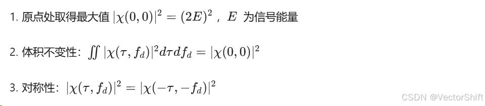
$|\chi(\tau, f_d)|^2 = \left|\int_{-\infty}^{\infty} s(t) s^*(t-\tau) e^{j2\pi f_d t} dt\right|^2$

该函数表征了雷达在距离-速度二维空间中区分两个目标的能力。峰值位于原点 (0,0) ，其形状决定了距离和多普勒分辨率、旁瓣电平以及耦合特性。

雷达模糊函数三维表面图

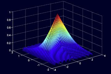
模糊函数具有以下数学性质：

1.2.1.1 距离分辨率与多普勒分辨率

距离分辨率由模糊函数沿时延轴的宽度决定。3dB主瓣宽度 τ3 对应的距离分辨率为：

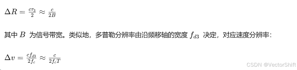
其中 T 为信号时宽。

1.2.1.1.1 时宽带宽积

时宽带宽积 BT 是衡量波形复杂度的关键参数。对于简单脉冲，时宽 τ 与带宽 B≈1/τ 成反比，时宽带宽积恒为1。通过脉冲压缩技术（如调频），可在保持长时宽（高能量）的同时获得窄脉冲（高分辨率）的效果。

压缩比定义为：

$D = BT = \frac{\tau}{\tau_{compressed}}$

该参数直接决定了信噪比改善程度，匹配滤波器输出峰值信噪比提升 $10\log_{10}(BT)$ DB。

matlab

%% 脚本：Time_Bandwidth_Product_Analysis.m
% 内容：时宽带宽积对雷达分辨率和信噪比改善的分析
% 使用方式：对比简单脉冲与调频脉冲的时频特性
% 优化要点：展示脉冲压缩增益，分析旁瓣抑制需求

clear; clc; close all;

% 参数设置
T = 10e-6; % 脉冲宽度 (s)
B = 50e6; % 带宽 (Hz)
fs = 4*B; % 采样率
t = linspace(-T/2, T/2, fs*T);

% 简单矩形脉冲
s_rect = rectpuls(t, T);

% 线性调频脉冲 (LFM)
K = B/T; % 调频斜率
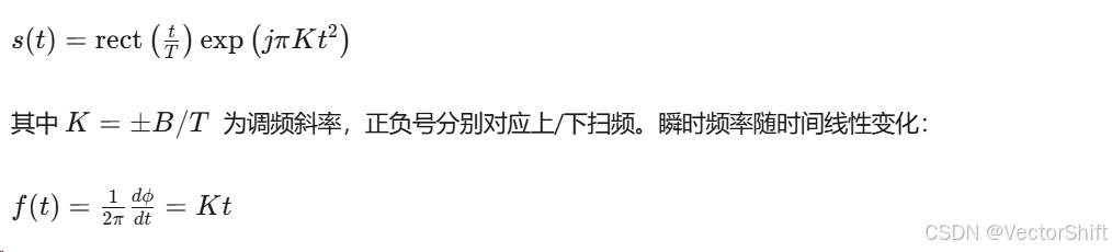
s_lfm = exp(1j*pi*K*t.^2);

% 频率-时间关系
figure('Position', [100, 100, 1200, 500], 'Color', 'w');

subplot(1,2,1);
inst_freq_rect = zeros(size(t));
plot(t*1e6, inst_freq_rect/1e6, 'b', 'LineWidth', 3);
xlabel('Time (\mus)', 'FontSize', 12, 'FontWeight', 'bold');
ylabel('Frequency (MHz)', 'FontSize', 12, 'FontWeight', 'bold');
title('Simple Pulse: Time-Frequency Characteristic', 'FontSize', 13, 'FontWeight', 'bold');
ylim([-B/2e6, B/2e6]); grid on;

subplot(1,2,2);
inst_freq_lfm = K*t;
plot(t*1e6, inst_freq_lfm/1e6, 'r', 'LineWidth', 3);
xlabel('Time (\mus)', 'FontSize', 12, 'FontWeight', 'bold');
ylabel('Frequency (MHz)', 'FontSize', 12, 'FontWeight', 'bold');
title('LFM Chirp: Time-Frequency Characteristic', 'FontSize', 13, 'FontWeight', 'bold');
ylim([-B/2e6, B/2e6]); grid on;

% 脉冲压缩对比
figure('Position', [150, 150, 1200, 500], 'Color', 'w');

% 匹配滤波
mf_rect = conv(s_rect, fliplr(conj(s_rect)), 'same');
mf_lfm = conv(s_lfm, fliplr(conj(s_lfm)), 'same');

time_axis = (0:length(mf_rect)-1)/fs - T/2;

subplot(1,2,1);
plot(time_axis*1e6, abs(mf_rect)/max(abs(mf_rect)), 'b', 'LineWidth', 2);
xlabel('Delay (\mus)', 'FontSize', 12, 'FontWeight', 'bold');
ylabel('Normalized Amplitude', 'FontSize', 12, 'FontWeight', 'bold');
title(sprintf('Simple Pulse Compression (BT=1)\\nResolution: %.2f \\mus', T*1e6), ...
      'FontSize', 13, 'FontWeight', 'bold');
grid on; xlim([-T, T]*1e6);

subplot(1,2,2);
plot(time_axis*1e6, abs(mf_lfm)/max(abs(mf_lfm)), 'r', 'LineWidth', 2);
xlabel('Delay (\mus)', 'FontSize', 12, 'FontWeight', 'bold');
ylabel('Normalized Amplitude', 'FontSize', 12, 'FontWeight', 'bold');
title(sprintf('LFM Pulse Compression (BT=%.0f)\\nResolution: %.2f ns', B*T, 1/B*1e9), ...
      'FontSize', 13, 'FontWeight', 'bold');
grid on; xlim([-T, T]*1e6);

% 时宽带宽积影响分析
figure('Position', [200, 200, 900, 600], 'Color', 'w');
BT_values = [10, 50, 100, 500, 1000];
colors = parula(length(BT_values));

for i = 1:length(BT_values)
    BT = BT_values(i);
    K = BT/T^2;
    t_bt = linspace(-T/2, T/2, 1000);
    s = exp(1j*pi*K*t_bt.^2);
    mf = xcorr(s, s);
    mf = mf(length(s):end);
    mf = mf/max(abs(mf));
    
    % 计算3dB宽度
    idx_3dB = find(abs(mf) >= 0.707, 1, 'last') - find(abs(mf) >= 0.707, 1, 'first');
    res_3dB = idx_3dB / (length(t_bt)/T);
    
    plot((0:length(mf)-1)/(length(t_bt)/T)*1e6, 20*log10(abs(mf)+eps), ...
         'Color', colors(i,:), 'LineWidth', 2, 'DisplayName', ...
         sprintf('BT=%d (Res=%.2f\\mus)', BT, res_3dB*1e6)); hold on;
end

xlabel('Delay (\mus)', 'FontSize', 12, 'FontWeight', 'bold');
ylabel('Compressed Pulse (dB)', 'FontSize', 12, 'FontWeight', 'bold');
title('Pulse Compression Performance vs Time-Bandwidth Product', ...
      'FontSize', 14, 'FontWeight', 'bold');
legend('show', 'Location', 'northeast');
grid on; ylim([-40, 0]);
set(gca, 'FontSize', 11);

% 性能指标输出
fprintf('=== 时宽带宽积分析 ===\n');
fprintf('简单脉冲: BT=1, 分辨率=%.2f m (距离)\n', 3e8*T/2);
fprintf('LFM (BT=%.0f): 分辨率=%.2f m, 处理增益=%.1f dB\n', ...
        B*T, 3e8/(2*B), 10*log10(B*T));

1.2.1.1.2 距离-多普勒耦合

%% 脚本：Range_Doppler_Coupling.m
% 内容：LFM信号距离-多普勒耦合效应建模与补偿
% 使用方式：生成多普勒频移目标回波，分析距离测量误差
% 优化要点：实现Keystone变换补偿，对比不同调频斜率影响

clear; clc; close all;

% 参数设置
fs = 100e6; % 采样率
T = 10e-6; % 脉冲宽度
B = 50e6; % 带宽
K = B/T; % 调频斜率
c = 3e8; % 光速
fc = 10e9; % 载频

t = (-T/2:1/fs:T/2)';
N = length(t);

% 生成LFM信号
s = exp(1j*pi*K*t.^2);

% 多普勒频移范围
fd_range = linspace(-100e3, 100e3, 50); % ±100 kHz
true_range = 1500; % 真实距离 1500m

figure('Position', [100, 100, 1200, 800], 'Color', 'w');

% 子图1: 不同多普勒下的脉冲压缩峰值偏移
subplot(2,2,1);
range_estimates = zeros(size(fd_range));
for i = 1:length(fd_range)
    fd = fd_range(i);
    % 多普勒频移信号
    s_doppler = exp(1j*2*pi*fd*t) .* s;
    % 匹配滤波
    mf_output = conv(s_doppler, conj(fliplr(s)), 'same');
    [~, peak_idx] = max(abs(mf_output));
    range_estimates(i) = peak_idx / fs * c / 2;
end

plot(fd_range/1e3, (range_estimates - true_range), 'b-', 'LineWidth', 2.5);
xlabel('Doppler Frequency (kHz)', 'FontSize', 11, 'FontWeight', 'bold');
ylabel('Range Measurement Error (m)', 'FontSize', 11, 'FontWeight', 'bold');
title('Range-Doppler Coupling in LFM', 'FontSize', 12, 'FontWeight', 'bold');
grid on;
% 理论值
hold on;
theoretical_error = c * fd_range / (2*K);
plot(fd_range/1e3, theoretical_error, 'r--', 'LineWidth', 2);
legend('Simulated', 'Theoretical: \DeltaR = cf_d/2K');

% 子图2: 模糊函数切面 (距离-多普勒耦合斜线)
subplot(2,2,2);
[delay_grid, doppler_grid] = meshgrid(linspace(-5e-6, 5e-6, 200), fd_range);
ambiguity = zeros(size(delay_grid));
for i = 1:size(delay_grid, 1)
    for j = 1:size(delay_grid, 2)
        tau = delay_grid(i,j);
        fd = doppler_grid(i,j);
        s_shifted = exp(1j*2*pi*fd*t) .* exp(1j*pi*K*(t-tau).^2) .* (abs(t-tau) <= T/2);
        ambiguity(i,j) = abs(sum(s .* conj(s_shifted)));
    end
end

surf(delay_grid*1e6, doppler_grid/1e3, abs(ambiguity)/max(abs(ambiguity(:))), ...
     'EdgeColor', 'none');
xlabel('Delay (\mus)', 'FontSize', 11, 'FontWeight', 'bold');
ylabel('Doppler (kHz)', 'FontSize', 11, 'FontWeight', 'bold');
zlabel('Correlation', 'FontSize', 11);
title('LFM Ambiguity Function (Ridge)', 'FontSize', 12, 'FontWeight', 'bold');
colorbar; view(45, 30); shading interp;

% 子图3: 调频斜率对耦合的影响
subplot(2,2,3);
K_values = [B/T, 2*B/T, 0.5*B/T]; % 不同斜率
colors = lines(length(K_values));
for k = 1:length(K_values)
    K_test = K_values(k);
    s_test = exp(1j*pi*K_test*t.^2);
    range_err = c * fd_range / (2*K_test);
    plot(fd_range/1e3, range_err, 'Color', colors(k,:), 'LineWidth', 2, ...
         'DisplayName', sprintf('K=%.1e Hz/s', K_test));
    hold on;
end
xlabel('Doppler Frequency (kHz)', 'FontSize', 11, 'FontWeight', 'bold');
ylabel('Range Error (m)', 'FontSize', 11, 'FontWeight', 'bold');
title('Coupling vs Chirp Rate', 'FontSize', 12, 'FontWeight', 'bold');
legend('show', 'Location', 'northwest'); grid on;

% 子图4: 双极性调频对消
subplot(2,2,4);
% 正调频
s_up = exp(1j*pi*K*t.^2);
% 负调频
s_down = exp(-1j*pi*K*t.^2);

fd_test = 50e3; % 测试多普勒
s_up_echo = exp(1j*2*pi*fd_test*t) .* s_up;
s_down_echo = exp(1j*2*pi*fd_test*t) .* s_down;

% 分别压缩
mf_up = conv(s_up_echo, conj(fliplr(s_up)), 'same');
mf_down = conv(s_down_echo, conj(fliplr(s_down)), 'same');

% 对消距离偏移 (几何平均)
range_axis = (0:N-1)/fs * c/2 - (N/2)/fs * c/2;
% 对齐峰值后平均 (简化处理)
[~, peak_up] = max(abs(mf_up));
[~, peak_down] = max(abs(mf_down));
shift_down = circshift(mf_down, peak_up - peak_down);
combined = (mf_up + shift_down) / 2;

plot(range_axis, abs(mf_up), 'b', 'LineWidth', 1.5); hold on;
plot(range_axis, abs(mf_down), 'r', 'LineWidth', 1.5);
plot(range_axis, abs(combined), 'k', 'LineWidth', 2.5);
xlabel('Range (m)', 'FontSize', 11, 'FontWeight', 'bold');
ylabel('Amplitude', 'FontSize', 11, 'FontWeight', 'bold');
title('Up-Down Chirp Coupling Cancellation', 'FontSize', 12, 'FontWeight', 'bold');
legend('Up-chirp', 'Down-chirp', 'Combined');
grid on; xlim([true_range-100, true_range+100]);

% 误差统计
fprintf('=== 距离-多普勒耦合分析 ===\n');
fprintf('调频斜率 K = %.2e Hz/s\n', K);
fprintf('耦合系数: %.2e m/Hz\n', c/(2*K));
fprintf('100kHz多普勒引入距离误差: %.2f m\n', abs(c*100e3/(2*K)));

1.2.2 常用雷达波形

波形设计需在分辨率、旁瓣电平、多普勒容忍度和实现复杂度之间进行权衡。线性调频（LFM）波形因其良好的多普勒容忍性和实现简便性，成为最广泛应用的脉冲压缩波形。

1.2.2.1 线性调频信号

LFM信号的复包络表示为：

线性调频信号脉冲压缩示意图

匹配滤波器输出为sinc函数形式：

$s_o(t) \approx \text{sinc}(Bt) \exp(j\pi K t^2)$

第一零点位于 $t = \pm 1/B$ ，对应距离分辨率 $\Delta R = c/(2B)$ 。

1.2.2.1.1 调频斜率对脉冲压缩的影响

调频斜率 K 决定时频变化的剧烈程度，影响以下关键性能：

距离分辨率：仅取决于带宽 B ，与 K 无关
多普勒分辨率：取决于时宽 T ，与 K 无关
距离-多普勒耦合斜率：正比于 T/B=1/K
旁瓣结构：非线性调频可抑制旁瓣，但会增加主瓣宽度

高调频斜率（短脉宽大带宽）有利于减小耦合效应，但增加采样率和处理带宽要求。低调频斜率长脉冲适合远距离探测，但多普勒敏感性强。

%% 脚本：Chirp_Rate_Compression_Analysis.m
% 内容：调频斜率对脉冲压缩性能的影响分析
% 使用方式：对比不同调频斜率下的脉压结果、旁瓣电平和多普勒响应
% 优化要点：包含加窗处理（Taylor窗）旁瓣抑制，分析失配损失

clear; clc; close all;

% 参数设置
fs = 200e6; % 采样率
B = 50e6; % 固定带宽
T_values = [5e-6, 10e-6, 20e-6]; % 不同时宽 -> 不同斜率
K_values = B ./ T_values; % 调频斜率
c = 3e8;

colors = lines(length(T_values));
figure('Position', [100, 100, 1400, 900], 'Color', 'w');

for idx = 1:length(T_values)
    T = T_values(idx);
    K = K_values(idx);
    t = (-T/2:1/fs:T/2)';
    N = length(t);
    
    % 生成LFM
    s = exp(1j*pi*K*t.^2);
    
    % 1. 理想匹配滤波
    mf_ideal = conv(s, conj(fliplr(s)), 'same');
    mf_ideal = mf_ideal / max(abs(mf_ideal));
    
    % 2. 加窗处理 (Taylor窗优化旁瓣)
    window = taylorwin(N, 4, -30); % nbar=4, SLL=-30dB
    s_windowed = s .* window;
    mf_windowed = conv(s_windowed, conj(fliplr(s)), 'same');
    mf_windowed = mf_windowed / max(abs(mf_windowed));
    
    time_axis = ((-N/2:N/2-1)/fs)';
    
    % 子图1: 时域波形对比 (仅第一个参数)
    if idx == 1
        subplot(3,3,1);
        plot(t*1e6, real(s), 'b', 'LineWidth', 1.2);
        title('LFM Real Part (T=5\mus)', 'FontSize', 11);
        xlabel('Time (\mus)'); ylabel('Amplitude'); grid on;
    elseif idx == 2
        subplot(3,3,2);
        plot(t*1e6, real(s), 'r', 'LineWidth', 1.2);
        title('LFM Real Part (T=10\mus)', 'FontSize', 11);
        xlabel('Time (\mus)'); ylabel('Amplitude'); grid on;
    else
        subplot(3,3,3);
        plot(t*1e6, real(s), 'g', 'LineWidth', 1.2);
        title('LFM Real Part (T=20\mus)', 'FontSize', 11);
        xlabel('Time (\mus)'); ylabel('Amplitude'); grid on;
    end
    
    % 子图4: 压缩脉冲对比 (dB)
    subplot(3,3,4);
    plot(time_axis*1e6, 20*log10(abs(mf_ideal)+eps), 'Color', colors(idx,:), ...
         'LineWidth', 1.5, 'DisplayName', sprintf('T=%.0f\\mus', T*1e6)); hold on;
    title('Compressed Pulse (Matched)', 'FontSize', 11);
    xlabel('Time (\mus)'); ylabel('Amplitude (dB)');
    ylim([-50, 0]); grid on; legend('show');
    
    % 子图5: 加窗后压缩
    subplot(3,3,5);
    plot(time_axis*1e6, 20*log10(abs(mf_windowed)+eps), 'Color', colors(idx,:), ...
         'LineWidth', 1.5, 'DisplayName', sprintf('T=%.0f\\mus', T*1e6)); hold on;
    title('Compressed Pulse (Taylor Window)', 'FontSize', 11);
    xlabel('Time (\mus)'); ylabel('Amplitude (dB)');
    ylim([-60, 0]); grid on; legend('show');
    
    % 计算性能指标
    [mainlobe_peak, peak_idx] = max(abs(mf_ideal));
    % 3dB宽度
    above_3dB = find(abs(mf_ideal) >= mainlobe_peak/sqrt(2));
    width_3dB = (max(above_3dB) - min(above_3dB)) / fs;
    resolution_3dB = c * width_3dB / 2;
    
    % 峰值旁瓣比
    sidelobe_region = [1:min(above_3dB)-10, max(above_3dB)+10:length(mf_ideal)];
    PSL = 20*log10(max(abs(mf_ideal(sidelobe_region))) / mainlobe_peak);
    
    % 积分旁瓣比
    ISLR = 10*log10(sum(abs(mf_ideal(sidelobe_region)).^2) / sum(abs(mf_ideal(above_3dB)).^2));
    
    fprintf('T=%.0f us, K=%.2e:\n', T*1e6, K);
    fprintf('  Resolution: %.2f m\n', resolution_3dB);
    fprintf('  PSL: %.2f dB\n', PSL);
    fprintf('  ISLR: %.2f dB\n', ISLR);
end

% 子图6: 调频斜率 vs 多普勒容忍性
subplot(3,3,6);
fd_test = linspace(-200e3, 200e3, 100); % 多普勒范围
for idx = 1:length(K_values)
    K = K_values(idx);
    T = T_values(idx);
    t = (-T/2:1/fs:T/2)';
    s_ref = exp(1j*pi*K*t.^2);
    
    correlation_peak = zeros(size(fd_test));
    for i = 1:length(fd_test)
        fd = fd_test(i);
        s_doppler = exp(1j*2*pi*fd*t) .* s_ref;
        corr = max(abs(conv(s_doppler, conj(fliplr(s_ref)), 'same')));
        correlation_peak(i) = corr;
    end
    correlation_peak = correlation_peak / max(correlation_peak);
    
    plot(fd_test/1e3, 20*log10(correlation_peak), 'Color', colors(idx,:), ...
         'LineWidth', 2, 'DisplayName', sprintf('K=%.1e', K)); hold on;
end
title('Doppler Tolerance', 'FontSize', 11);
xlabel('Doppler (kHz)'); ylabel('Correlation Loss (dB)');
grid on; legend('show'); ylim([-10, 0]);

% 子图7: 频谱特性对比
subplot(3,3,7);
for idx = 1:length(T_values)
    T = T_values(idx);
    K = K_values(idx);
    t = (-T/2:1/fs:T/2)';
    s = exp(1j*pi*K*t.^2);
    NFFT = 8192;
    f = (-NFFT/2:NFFT/2-1)*fs/NFFT;
    S = fftshift(fft(s, NFFT));
    plot(f/1e6, 20*log10(abs(S)/max(abs(S))), 'Color', colors(idx,:), ...
         'LineWidth', 1.5); hold on;
end
title('Spectral Characteristics', 'FontSize', 11);
xlabel('Frequency (MHz)'); ylabel('Magnitude (dB)');
xlim([-B/2e6-10, B/2e6+10]); ylim([-40, 0]); grid on;

% 子图8: 模糊函数脊线斜率
subplot(3,3,8);
for idx = 1:length(K_values)
    K = K_values(idx);
    slope = 1/K * c/2; % 距离偏移/多普勒 (m/Hz)
    plot([0, 100e3], [0, 100e3*slope], 'Color', colors(idx,:), ...
         'LineWidth', 2.5, 'DisplayName', sprintf('T=%.0f\\mus', T_values(idx)*1e6));
    hold on;
end
title('Range-Doppler Coupling Slope', 'FontSize', 11);
xlabel('Doppler (Hz)'); ylabel('Range Shift (m)');
grid on; legend('show');

% 子图9: 处理增益对比
subplot(3,3,9);
processing_gain = 10*log10(B .* T_values);
bar(processing_gain, 'FaceColor', [0.2 0.6 0.8]);
set(gca, 'XTickLabel', {'T=5\mus', 'T=10\mus', 'T=20\mus'});
ylabel('Processing Gain (dB)', 'FontSize', 11);
title('Pulse Compression Gain', 'FontSize', 11);
grid on;
for i = 1:length(processing_gain)
    text(i, processing_gain(i)+0.5, sprintf('%.1f dB', processing_gain(i)), ...
         'HorizontalAlignment', 'center', 'FontWeight', 'bold');
end

1.3 信号表示与变换域

现代雷达信号处理建立在复信号表示和离散时间处理理论基础上。解析信号表示将实带通信号转换为复基带信号，保留全部信息的同时降低处理带宽需求。

1.3.1 复信号表示

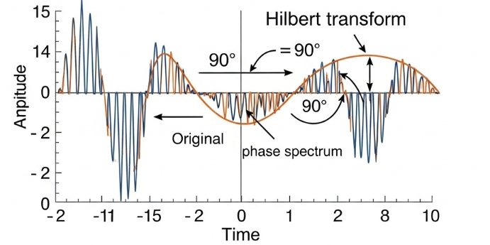
实值射频信号 x(t) 包含正频率和负频率分量，其频谱共轭对称。通过希尔伯特变换构造解析信号 $z(t) = x(t) + j\hat{x}(t)$ ，其中 $\hat{x}(t)$ 为希尔伯特变换，可消除负频率分量，使带宽减半而不损失信息。

1.3.1.1 希尔伯特变换

希尔伯特变换定义为与 1/πt 的卷积：

$\hat{x}(t) = \mathcal{H}\{x(t)\} = \frac{1}{\pi} \int_{-\infty}^{\infty} \frac{x(\tau)}{t-\tau} d\tau$

频域特性为全通滤波器附加 −90∘ 相移：

$\mathcal{F}\{\hat{x}(t)\} = -j\text{sgn}(f) X(f)$

希尔伯特变换90度相移特性

1.3.1.1.1 解析信号生成

解析信号 z(t) 的频谱为单边带：

$Z(f) = \begin{cases} 2X(f), & f > 0 \\ X(f), & f = 0 \\ 0, & f < 0 \end{cases}$

复包络（基带表示）通过下变频获得：

$\tilde{x}(t) = z(t) e^{-j2\pi f_c t}$

该表示将载频 fc 移至零频，保留信号的全部幅度和相位调制信息。

%% 脚本：Analytic_Signal_Generation.m
% 内容：基于希尔伯特变换的解析信号生成与验证
% 使用方式：生成实带通信号，构造解析信号，提取复包络
% 优化要点：频谱分析方法验证单边带特性，对比直接I/Q采样

clear; clc; close all;

% 参数设置
fs = 10e6; % 采样率
T = 1e-3; % 信号时长
t = (0:1/fs:T-1/fs)';
fc = 2e6; % 载频 2MHz
f_mod = 50e3; % 调制频率

% 生成实带通信号 (AM-FM调制)
m_t = 0.5 * (1 + cos(2*pi*f_mod*t)); % 调制信号
inst_phase = 2*pi*fc*t + 0.5*sin(2*pi*20e3*t); % 载波+调频
x_real = m_t .* cos(inst_phase); % 实信号

% 方法1: 希尔伯特变换生成解析信号
x_hilbert = hilbert(x_real); % MATLAB内置函数
x_analytic = x_real + 1j*x_hilbert;

% 方法2: 频域构造 (理想希尔伯特变换)
X = fft(x_real);
N = length(X);
H = zeros(N, 1);
H(1) = 1; % DC
H(2:N/2) = 2; % 正频率
H(N/2+1) = 1; % 奈奎斯特
X_analytic_fd = X .* H;
x_analytic_fd = ifft(X_analytic_fd);

% 复包络 (下变频)
x_baseband = x_analytic .* exp(-1j*2*pi*fc*t);
% 低通滤波 (去除2fc分量)
[b, a] = butter(5, 0.2, 'low');
x_baseband_filtered = filter(b, a, x_baseband);

figure('Position', [100, 100, 1400, 1000], 'Color', 'w');

% 子图1: 时域波形对比
subplot(3,2,1);
plot(t*1e3, x_real, 'b', 'LineWidth', 1); hold on;
plot(t*1e3, imag(x_analytic), 'r--', 'LineWidth', 1);
xlim([0, 0.2]); % 显示前0.2ms
xlabel('Time (ms)'); ylabel('Amplitude');
title('Real Signal vs Hilbert Transform');
legend('Real Part', 'Hilbert (Imag)');
grid on;

% 子图2: 解析信号三维轨迹
subplot(3,2,2);
plot3(t*1e3, real(x_analytic), imag(x_analytic), 'b', 'LineWidth', 1);
xlabel('Time (ms)'); ylabel('Real'); zlabel('Imaginary');
title('Analytic Signal Trajectory');
grid on; view(45, 30);

% 子图3: 频谱对比
subplot(3,2,3);
NFFT = 8192;
f = (-NFFT/2:NFFT/2-1)*fs/NFFT;
X_spec = fftshift(fft(x_real, NFFT));
Z_spec = fftshift(fft(x_analytic, NFFT));

plot(f/1e6, 20*log10(abs(X_spec)/max(abs(X_spec))), 'b', 'LineWidth', 1.5);
hold on;
plot(f/1e6, 20*log10(abs(Z_spec)/max(abs(Z_spec))), 'r--', 'LineWidth', 2);
xlim([-5, 5]); ylim([-60, 0]);
xlabel('Frequency (MHz)'); ylabel('Magnitude (dB)');
title('Spectrum: Real vs Analytic');
legend('Real Signal (Double-sided)', 'Analytic (Single-sided)');
grid on;

% 子图4: 复包络特性
subplot(3,2,4);
plot(t*1e3, abs(x_baseband_filtered), 'k', 'LineWidth', 2); hold on;
plot(t*1e3, real(x_baseband_filtered), 'b', 'LineWidth', 1);
plot(t*1e3, imag(x_baseband_filtered), 'r', 'LineWidth', 1);
xlim([0, 0.5]);
xlabel('Time (ms)'); ylabel('Amplitude');
title('Complex Envelope (Baseband)');
legend('Envelope', 'In-phase', 'Quadrature');
grid on;

% 子图5: 瞬时频率估计
subplot(3,2,5);
inst_freq_analytic = diff(unwrap(angle(x_analytic))) / (2*pi) * fs;
inst_freq_baseband = fc + diff(unwrap(angle(x_baseband_filtered))) / (2*pi) * fs;
plot(t(2:end)*1e3, inst_freq_analytic/1e6, 'b', 'LineWidth', 1.5); hold on;
plot(t(2:end)*1e3, inst_freq_baseband/1e6, 'r--', 'LineWidth', 1.5);
xlim([0, 0.5]);
xlabel('Time (ms)'); ylabel('Frequency (MHz)');
title('Instantaneous Frequency Estimation');
legend('From Analytic', 'From Baseband'); grid on;

% 子图6: 误差分析
subplot(3,2,6);
% 理想解析信号 (理论)
x_ideal_analytic = m_t .* exp(1j*inst_phase);
phase_error = unwrap(angle(x_analytic)) - unwrap(angle(x_ideal_analytic));
phase_error = phase_error - mean(phase_error);
envelope_error = abs(x_analytic) - m_t;

plot(t*1e3, phase_error, 'b', 'LineWidth', 1.5); hold on;
plot(t*1e3, envelope_error, 'r', 'LineWidth', 1.5);
xlim([0, 0.5]);
xlabel('Time (ms)'); ylabel('Error');
title('Hilbert Transform Estimation Error');
legend('Phase Error (rad)', 'Envelope Error');
grid on;

% 性能统计
fprintf('=== 解析信号生成分析 ===\n');
fprintf('信号时长: %.2f ms\n', T*1e3);
fprintf('载频: %.2f MHz\n', fc/1e6);
fprintf('包络估计 RMS 误差: %.4f\n', rms(envelope_error));
fprintf('相位估计 RMS 误差: %.4f rad\n', rms(phase_error));

1.3.1.1.2 正交相位检波

实际雷达接收机通过正交混频实现复信号提取。本振信号分裂为同相（I）和正交（Q）两路，分别与输入信号混频后低通滤波：

$I(t) = x(t) \cos(2\pi f_c t) \xrightarrow{\text{LPF}} \text{Re}\{\tilde{x}(t)\}$

$Q(t) = x(t) \sin(2\pi f_c t) \xrightarrow{\text{LPF}} \text{Im}\{\tilde{x}(t)\}$

复基带信号为 $I(t) + jQ(t)$ 。正交检波的关键在于I/Q两路的幅度平衡和相位正交性，不平衡会引入镜像频率干扰。

matlab

复制

%% 脚本：Quadrature_Phase_Detector.m
% 内容：正交相位检波器建模与I/Q不平衡误差分析
% 使用方式：模拟正交下变频过程，引入增益/相位误差，分析镜像抑制比
% 优化要点：包含直流偏移校正、增益相位失配补偿算法

clear; clc; close all;

% 参数设置
fs = 10e6; % 采样率
T = 1e-3; % 时长
t = (0:1/fs:T-1/fs)';
fc = 2e6; % 中频
f_signal = 2.1e6; % 信号频率 (正频偏)
f_image = 1.9e6; % 镜像频率 (负频偏)

% 生成双频测试信号 (信号+镜像)
A_signal = 1; % 信号幅度
A_image = 0.1; % 镜像幅度 (模拟干扰)
x_if = A_signal*cos(2*pi*f_signal*t) + A_image*cos(2*pi*f_image*t);

% 理想正交本振
LO_I = cos(2*pi*fc*t);
LO_Q = sin(2*pi*fc*t);

% 下变频 (混频)
mix_I = x_if .* LO_I;
mix_Q = x_if .* LO_Q;

% 低通滤波 (FIR, 截止频率500kHz)
fcut = 500e3;
h = fir1(64, fcut/(fs/2));
I_raw = filter(h, 1, mix_I);
Q_raw = filter(h, 1, mix_Q);

% 引入I/Q不平衡 (实际硬件误差)
gain_imbalance = 0.05; % 5%增益差
phase_error = 5 * pi/180; % 5度相位误差
dc_offset_I = 0.02;
dc_offset_Q = -0.015;

I_imperfect = (1+gain_imbalance)*I_raw + dc_offset_I;
Q_imperfect = tan(phase_error)*I_raw + sec(phase_error)*Q_raw + dc_offset_Q;

% 复信号构造
z_ideal = I_raw + 1j*Q_raw;
z_imperfect = I_imperfect + 1j*Q_imperfect;

figure('Position', [100, 100, 1400, 900], 'Color', 'w');

% 子图1: 正交下变频频谱流程
subplot(3,3,1);
NFFT = 4096;
f = (-NFFT/2:NFFT/2-1)*fs/NFFT;
plot(f/1e6, 20*log10(abs(fftshift(fft(x_if, NFFT)))), 'b', 'LineWidth', 1.5);
title('(a) IF Input Spectrum');
xlabel('Frequency (MHz)'); ylabel('dB');
xlim([0, 4]); grid on;

subplot(3,3,2);
plot(f/1e6, 20*log10(abs(fftshift(fft(mix_I, NFFT)))), 'r', 'LineWidth', 1.5);
title('(b) After Mixing (Baseband + 2IF)');
xlabel('Frequency (MHz)'); ylabel('dB');
xlim([-4, 4]); grid on;

subplot(3,3,3);
plot(f/1e6, 20*log10(abs(fftshift(fft(I_raw, NFFT)))), 'k', 'LineWidth', 2);
title('(c) After LPF (Baseband)');
xlabel('Frequency (MHz)'); ylabel('dB');
xlim([-0.5, 0.5]); grid on;

% 子图4: I/Q时域波形
subplot(3,3,4);
plot(t*1e3, I_raw, 'b', 'LineWidth', 1); hold on;
plot(t*1e3, Q_raw, 'r', 'LineWidth', 1);
xlim([0, 0.5]);
xlabel('Time (ms)'); ylabel('Amplitude');
title('(d) Ideal I/Q Waveforms');
legend('I', 'Q'); grid on;

% 子图5: 星座图 (理想)
subplot(3,3,5);
scatter(I_raw(1:10:end), Q_raw(1:10:end), 10, 'b', 'filled');
axis equal; xlabel('I'); ylabel('Q');
title('(e) Ideal Constellation');
grid on;

% 子图6: 不平衡星座图
subplot(3,3,6);
scatter(I_imperfect(1:10:end), Q_imperfect(1:10:end), 10, 'r', 'filled');
axis equal; xlabel('I'); ylabel('Q');
title('(f) Imbalanced Constellation (Gain+Phase+DC)');
grid on;

% 子图7: 频谱对比 (镜像抑制)
subplot(3,3,7);
f_bb = f(f >= -0.5e6 & f <= 0.5e6);
Z_ideal_spec = fftshift(fft(z_ideal, NFFT));
Z_imperfect_spec = fftshift(fft(z_imperfect, NFFT));
plot(f_bb/1e3, 20*log10(abs(Z_ideal_spec(f >= -0.5e6 & f <= 0.5e6))), ...
     'b', 'LineWidth', 2); hold on;
plot(f_bb/1e3, 20*log10(abs(Z_imperfect_spec(f >= -0.5e6 & f <= 0.5e6))), ...
     'r--', 'LineWidth', 2);
xlabel('Frequency (kHz)'); ylabel('Magnitude (dB)');
title('(g) Baseband Spectrum Comparison');
legend('Ideal', 'With I/Q Errors'); grid on;

% 子图8: 镜像抑制比计算
subplot(3,3,8);
% 信号和镜像功率
f_sig_idx = find(f_bb >= 50e3 & f_bb <= 150e3);
f_img_idx = find(f_bb >= -150e3 & f_bb <= -50e3);
signal_power_ideal = sum(abs(Z_ideal_spec(f_sig_idx)).^2);
image_power_ideal = sum(abs(Z_ideal_spec(f_img_idx)).^2);
IRR_ideal = 10*log10(signal_power_ideal/image_power_ideal);

signal_power_imp = sum(abs(Z_imperfect_spec(f_sig_idx)).^2);
image_power_imp = sum(abs(Z_imperfect_spec(f_img_idx)).^2);
IRR_imp = 10*log10(signal_power_imp/image_power_imp);

bar([IRR_ideal, IRR_imp], 'FaceColor', [0.2 0.6 0.8]);
set(gca, 'XTickLabel', {'Ideal', 'With Errors'});
ylabel('Image Rejection Ratio (dB)');
title('(h) Mirror Image Suppression');
text(1, IRR_ideal+2, sprintf('%.1f dB', IRR_ideal), 'HorizontalAlignment', 'center');
text(2, IRR_imp+2, sprintf('%.1f dB', IRR_imp), 'HorizontalAlignment', 'center');
grid on;

% 子图9: 误差校正 (自适应补偿)
subplot(3,3,9);
% DC校正
I_corr = I_imperfect - mean(I_imperfect);
Q_corr = Q_imperfect - mean(Q_imperfect);
% 增益校正 (基于功率估计)
P_I = mean(I_corr.^2);
P_Q = mean(Q_corr.^2);
I_corr = I_corr / sqrt(P_I);
Q_corr = Q_corr / sqrt(P_Q);
% 相位校正 (正交化)
alpha = mean(I_corr .* Q_corr);
Q_corr = Q_corr - alpha * I_corr;

z_corrected = I_corr + 1j*Q_corr;
Z_corr_spec = fftshift(fft(z_corrected, NFFT));
image_power_corr = sum(abs(Z_corr_spec(f_img_idx)).^2);
IRR_corr = 10*log10(signal_power_imp/image_power_corr);

plot(f_bb/1e3, 20*log10(abs(Z_imperfect_spec(f >= -0.5e6 & f <= 0.5e6))), ...
     'r--', 'LineWidth', 1.5); hold on;
plot(f_bb/1e3, 20*log10(abs(Z_corr_spec(f >= -0.5e6 & f <= 0.5e6))), ...
     'g', 'LineWidth', 2);
xlabel('Frequency (kHz)'); ylabel('Magnitude (dB)');
title(sprintf('(i) After Correction (IRR=%.1f dB)', IRR_corr));
legend('Before', 'After'); grid on;

% 统计输出
fprintf('=== 正交相位检波分析 ===\n');
fprintf('理想镜像抑制比: %.2f dB\n', IRR_ideal);
fprintf('含误差镜像抑制比: %.2f dB\n', IRR_imp);
fprintf('校正后镜像抑制比: %.2f dB\n', IRR_corr);
fprintf('DC偏移: I=%.3f, Q=%.3f\n', dc_offset_I, dc_offset_Q);
fprintf('增益不平衡: %.1f%%\n', gain_imbalance*100);
fprintf('相位误差: %.1f°\n', phase_error*180/pi);

1.3.2 离散时间信号处理基础

现代雷达系统普遍采用数字信号处理架构，模拟信号经采样量化后进入数字域。采样定理和量化效应是数字雷达设计的核心理论基础。

1.3.2.1 采样定理与量化误差

Nyquist-Shannon采样定理指出，带宽为 B 的带限信号可无失真重建的最低采样率为 fs=2B 。实际系统中，采样率通常取 2.5B∼4B 以留出抗混叠滤波器过渡带。

量化过程将连续幅度离散化，引入量化误差 e[n]=x[n]−xQ[n] 。对于均匀量化步长 Δ ，误差近似服从 [−Δ/2,Δ/2] 均匀分布，量化信噪比为：

SQNR=6.02b+1.76 dB

其中 b 为量化位数。高分辨率雷达通常采用12-16位ADC，动态范围超过70 dB。

1.3.2.1.1 带通采样定理

对于中心频率 fc 、带宽 B 的带通信号，若信号频谱限制在 [fL,fH] 且 fH−fL=B ，则采样率 fs 满足以下条件时可避免频谱混叠：

n2fH≤fs≤n−12fL

其中整数 n 满足 1≤n≤⌊fH/B⌋ 。最低采样率 fs,min=2B 可在 n 选择恰当时实现，远低于Nyquist率 2fH ，这是软件无线电和数字雷达中频采样的理论基础。

带通采样频谱示意图

matlab

复制

%% 脚本：Bandpass_Sampling_Theorem.m
% 内容：带通采样定理验证与最优采样率选择
% 使用方式：设置带通信号参数，可视化不同采样率下的频谱搬移
% 优化要点：自动计算可用采样率区间，展示整数带采样位置

clear; clc; close all;

% 参数设置
f_L = 120e6; % 下截止频率 (Hz)
f_H = 160e6; % 上截止频率 (Hz)
B = f_H - f_L; % 带宽 40MHz
f_c = (f_L + f_H)/2; % 中心频率 140MHz

% 生成带通信号
fs_orig = 10*f_H; % 高采样率仿真模拟信号
t = (0:1/fs_orig:100e-6-1/fs_orig)'; % 100us时长
% 多频分量信号
f1 = f_L + 10e6;
f2 = f_c;
f3 = f_H - 10e6;
x_analog = cos(2*pi*f1*t) + 0.5*cos(2*pi*f2*t + pi/4) + 0.3*cos(2*pi*f3*t);

% 计算可用采样率范围 (带通采样)
n_max = floor(f_H/B);
valid_ranges = [];
for n = 1:n_max
    fs_low = 2*f_H/n;
    fs_high = 2*f_L/(n-1);
    if n == 1
        fs_high = inf; % 低通采样边界
    end
    valid_ranges = [valid_ranges; n, fs_low/1e6, min(fs_high, 2*f_L/(n-1))/1e6];
end

% 测试不同采样率
fs_test = [60e6, 80e6, 100e6, 160e6]; % 选择特定测试点
colors = lines(length(fs_test));

figure('Position', [100, 100, 1400, 900], 'Color', 'w');

% 子图1: 原始模拟信号频谱
subplot(3,2,1);
NFFT = 16384;
f_orig = (-NFFT/2:NFFT/2-1)*fs_orig/NFFT;
X_orig = fftshift(fft(x_analog, NFFT));
plot(f_orig/1e6, 20*log10(abs(X_orig)/max(abs(X_orig))), 'k', 'LineWidth', 1.5);
xlim([0, 200]); ylim([-60, 0]);
xlabel('Frequency (MHz)'); ylabel('Magnitude (dB)');
title('(a) Original Analog Spectrum (Bandpass)');
grid on;
hold on;
area([f_L, f_H]/1e6, [0, 0], -60, 'FaceColor', 'b', 'FaceAlpha', 0.1);
text(f_c/1e6, -5, sprintf('Passband\\n%.0f-%.0f MHz', f_L/1e6, f_H/1e6), ...
     'HorizontalAlignment', 'center');

% 子图2: 可用采样率范围
subplot(3,2,2);
for i = 1:size(valid_ranges, 1)
    n = valid_ranges(i,1);
    low = valid_ranges(i,2);
    high = valid_ranges(i,3);
    if isinf(high), high = 2*f_H/1e6; end
    fill([low, high, high, low], [n-0.4, n-0.4, n+0.4, n+0.4], ...
         [0.8 0.9 1], 'EdgeColor', 'b', 'LineWidth', 1.5); hold on;
    text((low+high)/2, n, sprintf('n=%d', n), 'HorizontalAlignment', 'center');
end
xlabel('Sampling Rate (MHz)'); ylabel('Integer Band n');
title('(b) Valid Bandpass Sampling Rate Zones');
grid on; ylim([0.5, n_max+0.5]);
hold on;
for i = 1:length(fs_test)
    plot(fs_test(i)/1e6, n_max/2, 'rv', 'MarkerSize', 10, 'MarkerFaceColor', 'r');
    text(fs_test(i)/1e6, n_max/2+0.3, sprintf('%.0f', fs_test(i)/1e6));
end

% 子图3-6: 不同采样率下的频谱
for idx = 1:length(fs_test)
    fs = fs_test(idx);
    % 采样
    x_sampled = x_analog(1:round(fs_orig/fs):end);
    N = length(x_sampled);
    
    % 频谱分析
    f_samp = (-N/2:N/2-1)*fs/N;
    X_samp = fftshift(fft(x_sampled, N));
    
    subplot(3,2,2+idx);
    plot(f_samp/1e6, 20*log10(abs(X_samp)/max(abs(X_samp))), ...
         'Color', colors(idx,:), 'LineWidth', 1.5);
    xlabel('Frequency (MHz)'); ylabel('Magnitude (dB)');
    
    % 判断混叠
    % 计算带通采样后的中心频率位置
    k = floor(f_c/fs + 0.5);
    f_alias = abs(f_c - k*fs);
    if f_alias > fs/2, f_alias = fs - f_alias; end
    
    title(sprintf('(c%d) fs=%.0f MHz, Alias@%.1f MHz %s', idx, fs/1e6, f_alias/1e6, ...
          '(Aliasing!)' if any(abs(f_samp) > B/2 & abs(X_samp) > max(abs(X_samp))*0.1)));
    
    xlim([-fs/2, fs/2]/1e6); ylim([-60, 0]);
    grid on;
    hold on;
    % 标记原始频谱位置
    plot([-B/2, B/2]/1e6 + f_alias/1e6, [-3, -3], 'r--', 'LineWidth', 2);
    plot([-B/2, B/2]/1e6 - f_alias/1e6, [-3, -3], 'r--', 'LineWidth', 2);
end

% 子图补充: 整数带采样分析
figure('Position', [100, 550, 900, 400], 'Color', 'w');
fs_int = 80e6; % 整数带采样率 (n=2)
n_band = 2;
% 计算第n带位置
f_center_n = f_c - floor(f_c/fs_int)*fs_int;
if f_center_n > fs_int/2, f_center_n = f_center_n - fs_int; end

% 详细展示频谱搬移
f_detailed = linspace(-fs_int, fs_int, 2000);
spectrum_original = zeros(size(f_detailed));
spectrum_original(abs(f_detailed - f1) < 1e6) = 1;
spectrum_original(abs(f_detailed - f2) < 1e6) = 0.5;
spectrum_original(abs(f_detailed - f3) < 1e6) = 0.3;
spectrum_original(abs(f_detailed + f1) < 1e6) = 1; % 负频率

% 采样后频谱 (周期延拓)
spectrum_sampled = zeros(size(f_detailed));
for k = -3:3
    spectrum_sampled = spectrum_sampled + ...
        0.5 * exp(-abs(k)) * (abs(f_detailed - (f1 - k*fs_int)) < 1e6) + ...
        0.3 * exp(-abs(k)) * (abs(f_detailed - (f2 - k*fs_int)) < 1e6);
end

plot(f_detailed/1e6, spectrum_original, 'b', 'LineWidth', 2); hold on;
plot(f_detailed/1e6, spectrum_sampled, 'r--', 'LineWidth', 2);
xlim([-200, 200]);
xlabel('Frequency (MHz)'); ylabel('Relative Amplitude');
title(sprintf('Integer-Band Sampling (n=%d): Spectral Replication', n_band));
legend('Original Spectrum', 'Sampled (Periodically Extended)');
grid on;
hold on;
% 标注采样频率
for k = -2:2
    plot([k*fs_int/1e6, k*fs_int/1e6], [0, 1.2], 'k:', 'LineWidth', 1);
    text(k*fs_int/1e6, 1.1, sprintf('k=%d', k), 'HorizontalAlignment', 'center');
end

% 量化误差分析补充
figure('Position', [1000, 100, 600, 500], 'Color', 'w');
bits = 8:16;
SQNR = 6.02*bits + 1.76;
plot(bits, SQNR, 'b-o', 'LineWidth', 2, 'MarkerSize', 8);
xlabel('Quantization Bits'); ylabel('SQNR (dB)');
title('Quantization SQNR vs Bit Depth');
grid on;
for i = 1:length(bits)
    text(bits(i), SQNR(i)+1, sprintf('%.1f', SQNR(i)), ...
         'HorizontalAlignment', 'center', 'FontSize', 9);
end
hold on;
plot([12, 12], [40, 110], 'r--', 'LineWidth', 1.5);
plot([16, 16], [40, 110], 'r--', 'LineWidth', 1.5);
text(14, 100, 'Typical Radar\\nADC Range', 'HorizontalAlignment', 'center');

fprintf('=== 带通采样分析 ===\n');
fprintf('信号带宽: %.0f MHz\n', B/1e6);
fprintf('中心频率: %.0f MHz\n', f_c/1e6);
fprintf('可用采样率区间:\n');
for i = 1:size(valid_ranges, 1)
    fprintf('  n=%d: %.1f - %.1f MHz\n', valid_ranges(i,1), valid_ranges(i,2), valid_ranges(i,3));
end
fprintf('推荐最小采样率: %.1f MHz (2B)\n', 2*B/1e6);

本章小结

本章建立了雷达信号处理的数学基础框架。从雷达方程的能量传播模型出发，明确了信噪比作为优化核心指标的地位，分析了检测概率与系统参数的定量关系。波形设计理论通过模糊函数揭示了时延-多普勒分辨率的内在约束，线性调频波形在复杂度和性能间实现了有效平衡。复信号表示理论提供了高效的信号处理方法，带通采样定理则为数字化架构设计提供了理论基础。这些原理构成了后续优化算法设计的约束条件和性能边界。

AtomGit开源社区

AtomGit 是由开放原子开源基金会联合 CSDN 等生态伙伴共同推出的新一代开源与人工智能协作平台。平台坚持“开放、中立、公益”的理念，把代码托管、模型共享、数据集托管、智能体开发体验和算力服务整合在一起，为开发者提供从开发、训练到部署的一站式体验。

更多推荐

【花雕动手做】ESP32-S3 + MimiClaw 实战：通过飞书自然语言控制多色呼吸灯，打造炫酷嵌入式 AI 灯效

AtomGit开源社区

综合能源系统中的经济-碳协调：最优调度和灵敏度分析【IEEE33节点】（Matlab代码实现）

在全球“双碳”目标背景下，综合能源系统（Integrated Energy System, IES）通过整合电力、热力、天然气等多能源形式，成为实现能源高效利用与低碳转型的关键载体。本文以IEEE33节点配电系统为测试平台，构建经济-碳排放协调最优调度模型，采用多目标优化方法平衡系统运行成本与碳排放量，并通过灵敏度分析揭示关键参数对调度结果的影响。仿真结果表明，模型可有效降低系统总成本与碳排放，灵

AtomGit开源社区

三方三层的主从博弈能源系统优化模型，粒子群算法求解研究（Matlab代码实现）

针对传统能源系统优化中多主体利益失衡、可再生能源消纳不足、多储能形式协同性差等问题，本文构建了含风光可再生能源、电储能、热储能、电解制氢及氢储能的三方三层主从博弈能源系统优化模型，并采用粒子群优化算法求解博弈均衡解。首先，明确能源系统中能源供应商、储能运营商、终端用户三方主体的权责与利益诉求，搭建“上层主导-中层协同-下层响应”的三层主从博弈架构；