多物理场耦合仿真-主题062-代理模型与优化

kkchenkx

289人浏览 · 2026-03-29 10:04:13

kkchenkx · 2026-03-29 10:04:13 发布

主题062：代理模型与优化

摘要

代理模型（Surrogate Model）是现代工程优化中的核心技术，它通过构建计算成本低廉的近似模型来替代昂贵的高保真仿真，从而实现复杂系统的高效优化设计。随着工程问题复杂度的提升，单次仿真可能需要数小时甚至数天的计算时间，传统的直接优化方法面临计算不可行的困境。代理模型技术通过在设计空间中有策略地采样，建立输入-输出之间的近似映射关系，在保证精度的前提下将计算成本降低数个数量级。

本教程系统介绍代理模型的理论基础、核心方法和工程应用。首先阐述响应面方法（RSM）的数学原理和多项式拟合技术，包括线性和二次响应面模型的构建方法。其次详细介绍Kriging模型的统计基础、相关函数选择和超参数估计。然后讨论代理模型辅助优化的策略，包括序列优化和自适应采样方法。最后介绍多目标优化算法和Pareto前沿分析技术。通过Python实现六个典型案例，涵盖结构优化、热设计、流体系统等领域，展示代理模型在实际工程优化中的应用效果。

关键词：代理模型；响应面方法；Kriging模型；优化算法；序列优化；多目标优化；Pareto前沿；自适应采样

在这里插入图片描述

1. 引言

1.1 工程优化的挑战

在现代工程设计中，优化已成为提升产品性能、降低成本和缩短开发周期的关键手段。从航空航天器的轻量化设计到汽车发动机的燃烧效率优化，从微电子器件的热管理到建筑结构的抗震性能，工程优化问题无处不在。

然而，工程优化面临着一个根本性挑战：计算成本与优化效率的矛盾。以汽车外形气动优化为例：

单次CFD仿真需要8-12小时
一个设计变量需要评估数十个样本点
10个设计变量的优化可能需要数千次仿真
总计算时间将达到数年，这在实际工程中是不可接受的

这种困境被称为**“维度灾难”**（Curse of Dimensionality）：随着设计变量数量的增加，所需样本点数量呈指数增长。

1.2 代理模型的核心思想

代理模型技术的核心思想是：在设计空间中构建一个计算成本低廉的近似模型，用该模型替代昂贵的高保真仿真进行优化搜索。

代理模型的工作流程包括：

采样阶段：在设计空间中选择少量样本点（试验设计）
仿真阶段：执行高保真仿真获取样本响应
建模阶段：基于样本数据构建代理模型
优化阶段：在代理模型上进行优化搜索
验证阶段：验证最优解并更新模型（可选）

代理模型的优势：

计算效率：模型评估时间从小时级降至毫秒级
全局搜索：模型平滑性好，便于全局优化算法应用
不确定性量化：部分代理模型（如Kriging）提供预测不确定性估计
多目标处理：可方便地扩展到多目标优化问题

1.3 代理模型的发展历程

代理模型技术的发展经历了三个阶段：

经典响应面阶段（1950s-1980s）：Box和Wilson于1951年提出响应面方法（RSM），使用多项式函数近似黑箱函数。这是最早的系统代理建模方法，在化工、制药等领域得到广泛应用。

Kriging与随机过程阶段（1980s-2000s）：Sacks等人于1989年将地质统计学中的Kriging方法引入计算机实验设计。Kriging模型基于高斯随机过程，能够提供预测均值和方差，为基于不确定性的自适应采样奠定了基础。

机器学习融合阶段（2000s-至今）：神经网络、支持向量机等机器学习方法被应用于代理建模。特别是深度学习的发展，为高维复杂问题的代理建模提供了新工具。

1.4 本教程的内容安排

本教程从理论、方法和应用三个维度系统介绍代理模型与优化技术：

第2章阐述试验设计方法，包括拉丁超立方采样和正交试验设计，为代理模型构建提供高质量的样本数据。

第3章详细介绍响应面方法，包括线性和二次多项式模型、最小二乘拟合和方差分析。

第4章讨论Kriging模型，包括相关函数、超参数估计和预测不确定性。

第5章介绍代理模型辅助优化策略，包括序列优化、自适应采样和约束处理。

第6章讨论多目标优化算法，包括NSGA-II、Pareto前沿分析和决策方法。

第7章通过Python实现六个典型案例，涵盖RSM、Kriging、优化算法和多目标优化。

2. 试验设计方法

2.1 试验设计的重要性

试验设计（Design of Experiments, DOE）是代理模型构建的第一步，其目标是在设计空间中选择具有代表性的样本点。好的试验设计应该：

空间填充性：样本点均匀覆盖整个设计空间
投影均匀性：在低维投影上保持均匀分布
正交性：设计变量之间相关性最小
可扩展性：便于增加样本点进行模型更新

2.2 拉丁超立方采样

拉丁超立方采样（Latin Hypercube Sampling, LHS）是目前最常用的空间填充采样方法。它由McKay等人于1979年提出，结合了随机采样的灵活性和分层采样的均匀性。

LHS的基本原理：

对于 $d$ 维设计空间，每个维度被等分为 $n$ 个区间。LHS确保每个区间的每一行和每一列恰好有一个样本点，类似于拉丁方阵的结构。

LHS的生成算法：

对每个维度 $\ldots, d$ ：
- 生成随机排列 $πi\pi_i$ 的 $\ldots, n)$
对每个样本点 $\ldots, n$ ：
- 第 $i$ 维坐标： $xji=πi(j)−1+ujinx_{ji} = \frac{\pi_i(j) - 1 + u_{ji}}{n}$
- 其中 $uji∼U(0,1)u_{ji} \sim U(0, 1)$ 是均匀随机数

LHS的优势：

一维投影均匀：每个维度上样本点均匀分布
计算简单：易于实现和扩展
方差缩减：相比纯随机采样，估计方差更小

2.3 正交试验设计

正交试验设计基于正交表，能够在有限的试验次数下，全面考察多个因素对响应的影响。

正交表表示法： $L_n(q^d)$

$n$ ：试验次数（样本点数）
$q$ ：因素水平数
$d$ ：因素个数（设计变量数）

正交性的数学定义：

正交表的任意两列中，不同水平组合出现的次数相同。这保证了因素之间的独立性，便于分析各因素的主效应。

常用正交表：

$L_4(2^3)$ ：3个二水平因素，4次试验
$L_9(3^4)$ ：4个三水平因素，9次试验
$L_{16}(4^5)$ ：5个四水平因素，16次试验

2.4 Python实现：试验设计

import numpy as np
import matplotlib
matplotlib.use('Agg')
import matplotlib.pyplot as plt
from pyDOE2 import lhs
import os

plt.rcParams['font.sans-serif'] = ['SimHei', 'DejaVu Sans']
plt.rcParams['axes.unicode_minus'] = False

output_dir = os.path.join(os.path.dirname(__file__), 'output')
os.makedirs(output_dir, exist_ok=True)

# 定义设计空间维度
d = 2  # 2维设计空间
n_samples = 20  # 样本点数

# 方法1：随机采样
np.random.seed(42)
random_samples = np.random.rand(n_samples, d)

# 方法2：拉丁超立方采样
lhs_samples = lhs(d, samples=n_samples)

# 方法3：网格采样
n_grid = int(np.sqrt(n_samples))
x_grid = np.linspace(0, 1, n_grid)
y_grid = np.linspace(0, 1, n_grid)
X_grid, Y_grid = np.meshgrid(x_grid, y_grid)
grid_samples = np.column_stack([X_grid.flatten(), Y_grid.flatten()])

# 可视化对比
fig, axes = plt.subplots(1, 3, figsize=(15, 5))

# 随机采样
axes[0].scatter(random_samples[:, 0], random_samples[:, 1], c='blue', s=50, alpha=0.7)
axes[0].set_xlabel('设计变量 x₁', fontsize=11)
axes[0].set_ylabel('设计变量 x₂', fontsize=11)
axes[0].set_title('随机采样', fontsize=12)
axes[0].grid(True, alpha=0.3)
axes[0].set_xlim(0, 1)
axes[0].set_ylim(0, 1)

# 拉丁超立方采样
axes[1].scatter(lhs_samples[:, 0], lhs_samples[:, 1], c='red', s=50, alpha=0.7)
axes[1].set_xlabel('设计变量 x₁', fontsize=11)
axes[1].set_ylabel('设计变量 x₂', fontsize=11)
axes[1].set_title('拉丁超立方采样 (LHS)', fontsize=12)
axes[1].grid(True, alpha=0.3)
axes[1].set_xlim(0, 1)
axes[1].set_ylim(0, 1)

# 网格采样
axes[2].scatter(grid_samples[:, 0], grid_samples[:, 1], c='green', s=50, alpha=0.7)
axes[2].set_xlabel('设计变量 x₁', fontsize=11)
axes[2].set_ylabel('设计变量 x₂', fontsize=11)
axes[2].set_title('网格采样', fontsize=12)
axes[2].grid(True, alpha=0.3)
axes[2].set_xlim(0, 1)
axes[2].set_ylim(0, 1)

plt.tight_layout()
plt.savefig(os.path.join(output_dir, 'case1_sampling_methods.png'), dpi=150, bbox_inches='tight')
plt.close()

print("✓ 试验设计方法对比完成")

3. 响应面方法（RSM）

3.1 RSM的数学基础

响应面方法（Response Surface Methodology, RSM）使用多项式函数近似黑箱函数。最常用的模型形式包括：

一阶线性模型：
$y(x)=β0+∑i=1dβixi+ϵy(\mathbf{x}) = \beta_0 + \sum_{i=1}^{d} \beta_i x_i + \epsilon$

二阶二次模型：
$y(x)=β0+∑i=1dβixi+∑i=1dβiixi2+∑i<jβijxixj+ϵy(\mathbf{x}) = \beta_0 + \sum_{i=1}^{d} \beta_i x_i + \sum_{i=1}^{d} \beta_{ii} x_i^2 + \sum_{i<j} \beta_{ij} x_i x_j + \epsilon$

其中：

$y$ 是响应变量（目标函数值）
$x=[x1,x2,…,xd]T\mathbf{x} = [x_1, x_2, \ldots, x_d]^T$ 是设计变量
$β\beta$ 是待定系数
$ϵ\epsilon$ 是随机误差

3.2 最小二乘估计

给定 $n$ 个样本点 ${(x(i),y(i))}i=1n\{(\mathbf{x}^{(i)}, y^{(i)})\}_{i=1}^n$ ，系数 $β\boldsymbol{\beta}$ 通过最小二乘法估计：

$min⁡β∑i=1n(y(i)−f(x(i))Tβ)2\min_{\boldsymbol{\beta}} \sum_{i=1}^{n} \left(y^{(i)} - \mathbf{f}(\mathbf{x}^{(i)})^T \boldsymbol{\beta}\right)^2$

其中 $f(x)\mathbf{f}(\mathbf{x})$ 是基函数向量。

矩阵形式：

$y=Xβ+ϵ\mathbf{y} = \mathbf{X}\boldsymbol{\beta} + \boldsymbol{\epsilon}$

最小二乘解为：

$β^=(XTX)−1XTy\hat{\boldsymbol{\beta}} = (\mathbf{X}^T\mathbf{X})^{-1}\mathbf{X}^T\mathbf{y}$

3.3 模型评估与诊断

决定系数 $R^2$ ：

$R2=1−∑i=1n(y(i)−y^(i))2∑i=1n(y(i)−yˉ)2R^2 = 1 - \frac{\sum_{i=1}^{n}(y^{(i)} - \hat{y}^{(i)})^2}{\sum_{i=1}^{n}(y^{(i)} - \bar{y})^2}$

$R^2$ 越接近1，模型拟合越好。

调整 $R^2$ ：

$Radj2=1−n−1n−p(1−R2)R^2_{adj} = 1 - \frac{n-1}{n-p}(1 - R^2)$

其中 $p$ 是模型参数个数。调整 $R^2$ 考虑了模型复杂度，防止过拟合。

均方根误差（RMSE）：

$RMSE=1n∑i=1n(y(i)−y^(i))2RMSE = \sqrt{\frac{1}{n}\sum_{i=1}^{n}(y^{(i)} - \hat{y}^{(i)})^2}$

3.4 Python实现：响应面方法

import numpy as np
import matplotlib
matplotlib.use('Agg')
import matplotlib.pyplot as plt
from pyDOE2 import lhs
from sklearn.preprocessing import PolynomialFeatures
from sklearn.linear_model import LinearRegression
from sklearn.metrics import r2_score, mean_squared_error
import os

plt.rcParams['font.sans-serif'] = ['SimHei', 'DejaVu Sans']
plt.rcParams['axes.unicode_minus'] = False

output_dir = os.path.join(os.path.dirname(__file__), 'output')
os.makedirs(output_dir, exist_ok=True)

# 定义测试函数（Branin函数）
def branin(x):
    """Branin测试函数，具有多个局部最优"""
    x1, x2 = x[:, 0], x[:, 1]
    a = 1
    b = 5.1 / (4 * np.pi**2)
    c = 5 / np.pi
    r = 6
    s = 10
    t = 1 / (8 * np.pi)
    return a * (x2 - b*x1**2 + c*x1 - r)**2 + s*(1-t)*np.cos(x1) + s

# 设计空间
bounds = np.array([[-5, 10], [0, 15]])

# 生成训练样本
np.random.seed(42)
n_train = 30
X_train = lhs(2, samples=n_train)
X_train = bounds[:, 0] + X_train * (bounds[:, 1] - bounds[:, 0])
y_train = branin(X_train)

# 生成测试样本
n_test = 1000
X_test = np.random.rand(n_test, 2)
X_test = bounds[:, 0] + X_test * (bounds[:, 1] - bounds[:, 0])
y_test = branin(X_test)

# 构建响应面模型
# 线性模型
poly_linear = PolynomialFeatures(degree=1)
X_train_linear = poly_linear.fit_transform(X_train)
X_test_linear = poly_linear.transform(X_test)

model_linear = LinearRegression()
model_linear.fit(X_train_linear, y_train)
y_pred_linear = model_linear.predict(X_test_linear)

# 二次模型
poly_quad = PolynomialFeatures(degree=2)
X_train_quad = poly_quad.fit_transform(X_train)
X_test_quad = poly_quad.transform(X_test)

model_quad = LinearRegression()
model_quad.fit(X_train_quad, y_train)
y_pred_quad = model_quad.predict(X_test_quad)

# 评估模型
r2_linear = r2_score(y_test, y_pred_linear)
r2_quad = r2_score(y_test, y_pred_quad)
rmse_linear = np.sqrt(mean_squared_error(y_test, y_pred_linear))
rmse_quad = np.sqrt(mean_squared_error(y_test, y_pred_quad))

print(f"线性模型: R² = {r2_linear:.4f}, RMSE = {rmse_linear:.4f}")
print(f"二次模型: R² = {r2_quad:.4f}, RMSE = {rmse_quad:.4f}")

# 可视化
fig, axes = plt.subplots(2, 3, figsize=(15, 10))

# 真实函数
x1_grid = np.linspace(bounds[0, 0], bounds[0, 1], 100)
x2_grid = np.linspace(bounds[1, 0], bounds[1, 1], 100)
X1_grid, X2_grid = np.meshgrid(x1_grid, x2_grid)
X_grid = np.column_stack([X1_grid.flatten(), X2_grid.flatten()])
y_grid = branin(X_grid).reshape(X1_grid.shape)

ax = axes[0, 0]
im = ax.contourf(X1_grid, X2_grid, y_grid, levels=20, cmap='viridis')
ax.scatter(X_train[:, 0], X_train[:, 1], c='red', s=30, edgecolors='white')
ax.set_xlabel('x₁', fontsize=10)
ax.set_ylabel('x₂', fontsize=10)
ax.set_title('真实函数 (Branin)', fontsize=11)
plt.colorbar(im, ax=ax)

# 线性模型预测
y_linear_grid = model_linear.predict(poly_linear.transform(X_grid)).reshape(X1_grid.shape)
ax = axes[0, 1]
im = ax.contourf(X1_grid, X2_grid, y_linear_grid, levels=20, cmap='viridis')
ax.set_xlabel('x₁', fontsize=10)
ax.set_ylabel('x₂', fontsize=10)
ax.set_title(f'线性RSM (R²={r2_linear:.3f})', fontsize=11)
plt.colorbar(im, ax=ax)

# 二次模型预测
y_quad_grid = model_quad.predict(poly_quad.transform(X_grid)).reshape(X1_grid.shape)
ax = axes[0, 2]
im = ax.contourf(X1_grid, X2_grid, y_quad_grid, levels=20, cmap='viridis')
ax.set_xlabel('x₁', fontsize=10)
ax.set_ylabel('x₂', fontsize=10)
ax.set_title(f'二次RSM (R²={r2_quad:.3f})', fontsize=11)
plt.colorbar(im, ax=ax)

# 线性模型误差
ax = axes[1, 0]
error_linear = np.abs(y_grid - y_linear_grid)
im = ax.contourf(X1_grid, X2_grid, error_linear, levels=20, cmap='hot')
ax.set_xlabel('x₁', fontsize=10)
ax.set_ylabel('x₂', fontsize=10)
ax.set_title('线性模型绝对误差', fontsize=11)
plt.colorbar(im, ax=ax)

# 二次模型误差
ax = axes[1, 1]
error_quad = np.abs(y_grid - y_quad_grid)
im = ax.contourf(X1_grid, X2_grid, error_quad, levels=20, cmap='hot')
ax.set_xlabel('x₁', fontsize=10)
ax.set_ylabel('x₂', fontsize=10)
ax.set_title('二次模型绝对误差', fontsize=11)
plt.colorbar(im, ax=ax)

# 预测vs真实值
ax = axes[1, 2]
ax.scatter(y_test, y_pred_linear, c='blue', alpha=0.5, label='线性模型', s=20)
ax.scatter(y_test, y_pred_quad, c='red', alpha=0.5, label='二次模型', s=20)
ax.plot([y_test.min(), y_test.max()], [y_test.min(), y_test.max()], 'k--', lw=2)
ax.set_xlabel('真实值', fontsize=10)
ax.set_ylabel('预测值', fontsize=10)
ax.set_title('预测值 vs 真实值', fontsize=11)
ax.legend()
ax.grid(True, alpha=0.3)

plt.tight_layout()
plt.savefig(os.path.join(output_dir, 'case2_response_surface.png'), dpi=150, bbox_inches='tight')
plt.close()
print("✓ 响应面方法完成")

4. Kriging模型

4.1 Kriging的统计基础

Kriging模型（也称为高斯过程回归）将黑箱函数视为高斯随机过程的实现。与确定性响应面不同，Kriging提供预测均值和预测方差，为基于不确定性的优化提供了理论基础。

Kriging模型假设：

$y(x)=μ(x)+Z(x)y(\mathbf{x}) = \mu(\mathbf{x}) + Z(\mathbf{x})$

其中：

$μ(x)\mu(\mathbf{x})$ 是趋势函数（通常取常数或多项式）
$Z(x)Z(\mathbf{x})$ 是零均值高斯随机过程，协方差函数为：

$Cov[Z(x),Z(x′)]=σ2R(x,x′)\text{Cov}[Z(\mathbf{x}), Z(\mathbf{x}')] = \sigma^2 R(\mathbf{x}, \mathbf{x}')$

$R(x,x′)R(\mathbf{x}, \mathbf{x}')$ 是相关函数，描述两点之间的空间相关性。

4.2 相关函数

相关函数的选择对Kriging模型性能至关重要。常用相关函数包括：

高斯相关函数：
$R(x,x′)=exp⁡(−∑i=1dθi(xi−xi′)2)R(\mathbf{x}, \mathbf{x}') = \exp\left(-\sum_{i=1}^{d} \theta_i (x_i - x_i')^2\right)$

指数相关函数：
$R(x,x′)=exp⁡(−∑i=1dθi∣xi−xi′∣)R(\mathbf{x}, \mathbf{x}') = \exp\left(-\sum_{i=1}^{d} \theta_i |x_i - x_i'|\right)$

Matérn相关函数（更一般形式）：
$R(x,x′)=1Γ(ν)2ν−1(2ν∣x−x′∣θ)νKν(2ν∣x−x′∣θ)R(\mathbf{x}, \mathbf{x}') = \frac{1}{\Gamma(\nu)2^{\nu-1}} \left(\frac{2\sqrt{\nu}|\mathbf{x}-\mathbf{x}'|}{\theta}\right)^{\nu} K_{\nu}\left(\frac{2\sqrt{\nu}|\mathbf{x}-\mathbf{x}'|}{\theta}\right)$

其中 $θi\theta_i$ 是超参数，控制相关性的衰减速率。

4.3 Kriging预测

给定样本数据，Kriging预测公式为：

预测均值：
$y^(x)=μ^+r(x)TR−1(y−μ^1)\hat{y}(\mathbf{x}) = \hat{\mu} + \mathbf{r}(\mathbf{x})^T \mathbf{R}^{-1}(\mathbf{y} - \hat{\mu}\mathbf{1})$

预测方差：
$σ^2(x)=σ2[1−r(x)TR−1r(x)+(1−1TR−1r(x))21TR−11]\hat{\sigma}^2(\mathbf{x}) = \sigma^2 \left[1 - \mathbf{r}(\mathbf{x})^T \mathbf{R}^{-1}\mathbf{r}(\mathbf{x}) + \frac{(1 - \mathbf{1}^T\mathbf{R}^{-1}\mathbf{r}(\mathbf{x}))^2}{\mathbf{1}^T\mathbf{R}^{-1}\mathbf{1}}\right]$

其中：

$R\mathbf{R}$ 是样本点之间的相关矩阵
$r(x)\mathbf{r}(\mathbf{x})$ 是预测点与样本点的相关向量
$μ^\hat{\mu}$ 是趋势系数估计

4.4 超参数估计

超参数 $θ\boldsymbol{\theta}$ 通过最大似然估计（MLE）确定：

$max⁡θL(θ)=−n2ln⁡(σ^2)−12ln⁡∣R∣\max_{\boldsymbol{\theta}} L(\boldsymbol{\theta}) = -\frac{n}{2}\ln(\hat{\sigma}^2) - \frac{1}{2}\ln|\mathbf{R}|$

其中：
$σ^2=(y−μ^1)TR−1(y−μ^1)n\hat{\sigma}^2 = \frac{(\mathbf{y} - \hat{\mu}\mathbf{1})^T\mathbf{R}^{-1}(\mathbf{y} - \hat{\mu}\mathbf{1})}{n}$

4.5 Python实现：Kriging模型

import numpy as np
import matplotlib
matplotlib.use('Agg')
import matplotlib.pyplot as plt
from pyDOE2 import lhs
from sklearn.metrics import r2_score, mean_squared_error
from scipy.optimize import minimize
import os

plt.rcParams['font.sans-serif'] = ['SimHei', 'DejaVu Sans']
plt.rcParams['axes.unicode_minus'] = False

output_dir = os.path.join(os.path.dirname(__file__), 'output')
os.makedirs(output_dir, exist_ok=True)

# 定义测试函数（Hartmann 3D）
def hartmann3(x):
    """Hartmann 3D测试函数"""
    alpha = np.array([1.0, 1.2, 3.0, 3.2])
    A = np.array([[3.0, 10, 30],
                  [0.1, 10, 35],
                  [3.0, 10, 30],
                  [0.1, 10, 35]])
    P = 1e-4 * np.array([[3689, 1170, 2673],
                         [4699, 4387, 7470],
                         [1091, 8732, 5547],
                         [381, 5743, 8828]])
    
    y = 0
    for i in range(4):
        inner = 0
        for j in range(3):
            inner += A[i, j] * (x[:, j] - P[i, j])**2
        y += alpha[i] * np.exp(-inner)
    return -y

# 高斯相关函数
def gaussian_correlation(X1, X2, theta):
    """计算高斯相关矩阵"""
    n1, d = X1.shape
    n2 = X2.shape[0]
    R = np.zeros((n1, n2))
    
    for i in range(n1):
        for j in range(n2):
            diff = X1[i] - X2[j]
            R[i, j] = np.exp(-np.sum(theta * diff**2))
    return R

# Kriging模型类
class KrigingModel:
    def __init__(self, theta0=None):
        self.theta = theta0
        self.X_train = None
        self.y_train = None
        self.mu = None
        self.sigma2 = None
        self.R_inv = None
        
    def fit(self, X, y):
        self.X_train = X.copy()
        self.y_train = y.copy()
        n, d = X.shape
        
        # 如果未指定theta，使用MLE估计
        if self.theta is None:
            def neg_log_likelihood(theta):
                R = gaussian_correlation(X, X, theta) + 1e-10 * np.eye(n)
                try:
                    R_inv = np.linalg.inv(R)
                except:
                    return 1e10
                
                ones = np.ones(n)
                mu = (ones @ R_inv @ y) / (ones @ R_inv @ ones)
                sigma2 = ((y - mu) @ R_inv @ (y - mu)) / n
                
                if sigma2 <= 0:
                    return 1e10
                
                return n * np.log(sigma2) + np.log(np.linalg.det(R))
            
            # 优化超参数
            bounds = [(1e-3, 10) for _ in range(d)]
            result = minimize(neg_log_likelihood, np.ones(d), 
                            method='L-BFGS-B', bounds=bounds)
            self.theta = result.x
        
        # 计算相关矩阵
        R = gaussian_correlation(X, X, self.theta) + 1e-10 * np.eye(n)
        self.R_inv = np.linalg.inv(R)
        
        # 估计趋势系数
        ones = np.ones(n)
        self.mu = (ones @ self.R_inv @ y) / (ones @ self.R_inv @ ones)
        
        # 估计过程方差
        self.sigma2 = ((y - self.mu) @ self.R_inv @ (y - self.mu)) / n
        
    def predict(self, X, return_std=False):
        n_train = self.X_train.shape[0]
        n_test = X.shape[0]
        
        # 计算相关向量
        r = gaussian_correlation(X, self.X_train, self.theta)
        
        # 预测均值
        y_pred = self.mu + r @ self.R_inv @ (self.y_train - self.mu)
        
        if return_std:
            # 预测方差
            ones = np.ones(n_train)
            u = ones @ self.R_inv @ r.T
            
            r_self = np.array([gaussian_correlation(X[i:i+1], X[i:i+1], self.theta)[0, 0] 
                              for i in range(n_test)])
            
            sigma2_pred = self.sigma2 * (1 - np.sum(r * (self.R_inv @ r.T).T, axis=1) + 
                                        (1 - u)**2 / (ones @ self.R_inv @ ones))
            sigma2_pred = np.maximum(sigma2_pred, 0)
            return y_pred, np.sqrt(sigma2_pred)
        
        return y_pred

# 生成数据
np.random.seed(42)
n_train = 50
n_test = 500

X_train = lhs(3, samples=n_train)
y_train = hartmann3(X_train)

X_test = np.random.rand(n_test, 3)
y_test = hartmann3(X_test)

# 训练Kriging模型
print("训练Kriging模型...")
kriging = KrigingModel()
kriging.fit(X_train, y_train)
print(f"最优超参数 theta: {kriging.theta}")

# 预测
y_pred_kriging, y_std = kriging.predict(X_test, return_std=True)

# 评估
r2_kriging = r2_score(y_test, y_pred_kriging)
rmse_kriging = np.sqrt(mean_squared_error(y_test, y_pred_kriging))

print(f"Kriging模型: R² = {r2_kriging:.4f}, RMSE = {rmse_kriging:.4f}")

# 可视化
fig, axes = plt.subplots(2, 2, figsize=(12, 10))

# 预测vs真实值
ax = axes[0, 0]
ax.scatter(y_test, y_pred_kriging, c='blue', alpha=0.5, s=20)
ax.plot([y_test.min(), y_test.max()], [y_test.min(), y_test.max()], 'r--', lw=2)
ax.set_xlabel('真实值', fontsize=11)
ax.set_ylabel('预测值', fontsize=11)
ax.set_title(f'Kriging预测 (R²={r2_kriging:.3f})', fontsize=12)
ax.grid(True, alpha=0.3)

# 预测误差分布
ax = axes[0, 1]
errors = y_test - y_pred_kriging
ax.hist(errors, bins=30, color='steelblue', alpha=0.7, edgecolor='black')
ax.axvline(x=0, color='red', linestyle='--', linewidth=2)
ax.set_xlabel('预测误差', fontsize=11)
ax.set_ylabel('频数', fontsize=11)
ax.set_title('预测误差分布', fontsize=12)
ax.grid(True, alpha=0.3)

# 预测标准差
ax = axes[1, 0]
ax.scatter(y_std, np.abs(errors), c='green', alpha=0.5, s=20)
ax.set_xlabel('预测标准差', fontsize=11)
ax.set_ylabel('绝对误差', fontsize=11)
ax.set_title('预测不确定性 vs 实际误差', fontsize=12)
ax.grid(True, alpha=0.3)

# 残差图
ax = axes[1, 1]
ax.scatter(y_pred_kriging, errors, c='purple', alpha=0.5, s=20)
ax.axhline(y=0, color='red', linestyle='--', linewidth=2)
ax.set_xlabel('预测值', fontsize=11)
ax.set_ylabel('残差', fontsize=11)
ax.set_title('残差图', fontsize=12)
ax.grid(True, alpha=0.3)

plt.tight_layout()
plt.savefig(os.path.join(output_dir, 'case3_kriging_model.png'), dpi=150, bbox_inches='tight')
plt.close()
print("✓ Kriging模型完成")

5. 代理模型辅助优化

5.1 优化问题描述

考虑一般约束优化问题：

$min⁡xf(x)\min_{\mathbf{x}} f(\mathbf{x})$

约束条件：
$gi(x)≤0,i=1,2,…,mg_i(\mathbf{x}) \leq 0, \quad i = 1, 2, \ldots, m$
$hj(x)=0,j=1,2,…,ph_j(\mathbf{x}) = 0, \quad j = 1, 2, \ldots, p$
$xL≤x≤xU\mathbf{x}_L \leq \mathbf{x} \leq \mathbf{x}_U$

其中 $f(x)f(\mathbf{x})$ 是目标函数，通常需要通过昂贵的高保真仿真评估。

5.2 序列优化策略

序列优化（Sequential Optimization）通过迭代更新代理模型逐步逼近最优解：

初始化：使用试验设计生成初始样本
循环直到收敛：
- 构建/更新代理模型
- 在代理模型上求解优化问题
- 在最优点执行高保真仿真
- 添加新样本并检查收敛

收敛准则：

连续多次迭代目标函数改进小于阈值
代理模型预测误差小于阈值
达到最大迭代次数

5.3 自适应采样

自适应采样（Adaptive Sampling）根据代理模型的不确定性指导新样本的选择：

期望改进（Expected Improvement, EI）：

$EI(x)=E[max⁡(fmin−Y(x),0)]EI(\mathbf{x}) = E[\max(f_{min} - Y(\mathbf{x}), 0)]$

其中 $Y(x)Y(\mathbf{x})$ 是Kriging模型在 $x\mathbf{x}$ 处的随机预测， $f_{min}$ 是当前最优值。

对于Kriging模型，EI有解析表达式：

$EI(x)=(fmin−y^(x))Φ(fmin−y^(x)σ^(x))+σ^(x)ϕ(fmin−y^(x)σ^(x))EI(\mathbf{x}) = (f_{min} - \hat{y}(\mathbf{x}))\Phi\left(\frac{f_{min} - \hat{y}(\mathbf{x})}{\hat{\sigma}(\mathbf{x})}\right) + \hat{\sigma}(\mathbf{x})\phi\left(\frac{f_{min} - \hat{y}(\mathbf{x})}{\hat{\sigma}(\mathbf{x})}\right)$

其中 $Φ\Phi$ 和 $ϕ\phi$ 分别是标准正态分布的CDF和PDF。

5.4 Python实现：代理模型优化

import numpy as np
import matplotlib
matplotlib.use('Agg')
import matplotlib.pyplot as plt
from pyDOE2 import lhs
from scipy.optimize import minimize
from scipy.stats import norm
import os

plt.rcParams['font.sans-serif'] = ['SimHei', 'DejaVu Sans']
plt.rcParams['axes.unicode_minus'] = False

output_dir = os.path.join(os.path.dirname(__file__), 'output')
os.makedirs(output_dir, exist_ok=True)

# 定义昂贵目标函数（模拟）
def expensive_function(x):
    """模拟昂贵函数：带噪声的多峰函数"""
    x1, x2 = x[:, 0], x[:, 1]
    # 基础函数
    f = (x1**2 + x2 - 11)**2 + (x1 + x2**2 - 7)**2
    # 添加高频成分（模拟仿真噪声）
    f += 5 * np.sin(3*x1) * np.cos(3*x2)
    return f

# 简化的Kriging模型（复用前面的实现）
class SimpleKriging:
    def __init__(self, theta=0.5):
        self.theta = theta
        self.X_train = None
        self.y_train = None
        self.mu = None
        self.R_inv = None
        
    def correlation(self, X1, X2):
        n1, d = X1.shape
        n2 = X2.shape[0]
        R = np.zeros((n1, n2))
        for i in range(n1):
            for j in range(n2):
                R[i, j] = np.exp(-self.theta * np.sum((X1[i] - X2[j])**2))
        return R
        
    def fit(self, X, y):
        self.X_train = X.copy()
        self.y_train = y.copy()
        n = X.shape[0]
        
        R = self.correlation(X, X) + 1e-6 * np.eye(n)
        self.R_inv = np.linalg.inv(R)
        
        ones = np.ones(n)
        self.mu = (ones @ self.R_inv @ y) / (ones @ self.R_inv @ ones)
        
    def predict(self, X, return_std=False):
        r = self.correlation(X, self.X_train)
        y_pred = self.mu + r @ self.R_inv @ (self.y_train - self.mu)
        
        if return_std:
            n_train = self.X_train.shape[0]
            ones = np.ones(n_train)
            r_self = np.ones(X.shape[0])
            u = ones @ self.R_inv @ r.T
            sigma2 = 1 - np.sum(r * (self.R_inv @ r.T).T, axis=1) + (1 - u)**2 / (ones @ self.R_inv @ ones)
            sigma2 = np.maximum(sigma2, 0)
            return y_pred, np.sqrt(sigma2)
        return y_pred

# 期望改进函数
def expected_improvement(X, model, f_min):
    y_pred, y_std = model.predict(X, return_std=True)
    y_std = np.maximum(y_std, 1e-9)
    
    z = (f_min - y_pred) / y_std
    ei = (f_min - y_pred) * norm.cdf(z) + y_std * norm.pdf(z)
    return ei

# 序列优化
np.random.seed(42)
bounds = np.array([[-5, 5], [-5, 5]])

# 初始样本
n_init = 10
X_train = lhs(2, samples=n_init)
X_train = bounds[:, 0] + X_train * (bounds[:, 1] - bounds[:, 0])
y_train = expensive_function(X_train)

# 存储优化历史
history_X = [X_train.copy()]
history_y = [y_train.copy()]
history_best = [y_train.min()]

# 序列优化循环
n_iterations = 15
print("开始序列优化...")

for iteration in range(n_iterations):
    # 构建Kriging模型
    model = SimpleKriging(theta=0.5)
    model.fit(X_train, y_train)
    
    # 当前最优值
    f_min = y_train.min()
    
    # 在代理模型上寻找期望改进最大的点
    def neg_ei(x):
        x = x.reshape(1, -1)
        return -expected_improvement(x, model, f_min)[0]
    
    # 多起点优化
    best_ei = -np.inf
    best_x = None
    for _ in range(10):
        x0 = np.random.uniform(bounds[:, 0], bounds[:, 1])
        result = minimize(neg_ei, x0, method='L-BFGS-B', 
                         bounds=[(bounds[i, 0], bounds[i, 1]) for i in range(2)])
        if -result.fun > best_ei:
            best_ei = -result.fun
            best_x = result.x
    
    # 在最优点执行昂贵仿真
    y_new = expensive_function(best_x.reshape(1, -1))
    
    # 更新训练数据
    X_train = np.vstack([X_train, best_x])
    y_train = np.append(y_train, y_new)
    
    # 记录历史
    history_X.append(X_train.copy())
    history_y.append(y_train.copy())
    history_best.append(y_train.min())
    
    print(f"迭代 {iteration+1}: 最优值 = {y_train.min():.4f}, EI = {best_ei:.4f}")

# 可视化优化过程
fig, axes = plt.subplots(2, 3, figsize=(15, 10))

# 真实函数
x1_grid = np.linspace(bounds[0, 0], bounds[0, 1], 100)
x2_grid = np.linspace(bounds[1, 0], bounds[1, 1], 100)
X1_grid, X2_grid = np.meshgrid(x1_grid, x2_grid)
X_grid = np.column_stack([X1_grid.flatten(), X2_grid.flatten()])
y_grid = expensive_function(X_grid).reshape(X1_grid.shape)

ax = axes[0, 0]
im = ax.contourf(X1_grid, X2_grid, y_grid, levels=20, cmap='viridis')
ax.scatter(X_train[:, 0], X_train[:, 1], c='red', s=50, edgecolors='white', zorder=5)
ax.set_xlabel('x₁', fontsize=10)
ax.set_ylabel('x₂', fontsize=10)
ax.set_title('真实函数与采样点', fontsize=11)
plt.colorbar(im, ax=ax)

# 最终代理模型
model_final = SimpleKriging(theta=0.5)
model_final.fit(X_train, y_train)
y_pred_grid = model_final.predict(X_grid).reshape(X1_grid.shape)

ax = axes[0, 1]
im = ax.contourf(X1_grid, X2_grid, y_pred_grid, levels=20, cmap='viridis')
ax.scatter(X_train[:, 0], X_train[:, 1], c='red', s=50, edgecolors='white', zorder=5)
ax.set_xlabel('x₁', fontsize=10)
ax.set_ylabel('x₂', fontsize=10)
ax.set_title('最终代理模型', fontsize=11)
plt.colorbar(im, ax=ax)

# 期望改进
ax = axes[0, 2]
ei_grid = expected_improvement(X_grid, model_final, y_train.min()).reshape(X1_grid.shape)
im = ax.contourf(X1_grid, X2_grid, ei_grid, levels=20, cmap='hot')
ax.scatter(X_train[:, 0], X_train[:, 1], c='blue', s=50, edgecolors='white', zorder=5)
ax.set_xlabel('x₁', fontsize=10)
ax.set_ylabel('x₂', fontsize=10)
ax.set_title('期望改进 (EI)', fontsize=11)
plt.colorbar(im, ax=ax)

# 收敛历史
ax = axes[1, 0]
ax.plot(range(len(history_best)), history_best, 'b-o', linewidth=2, markersize=6)
ax.set_xlabel('迭代次数', fontsize=11)
ax.set_ylabel('最优目标值', fontsize=11)
ax.set_title('优化收敛历史', fontsize=12)
ax.grid(True, alpha=0.3)

# 样本点数量
ax = axes[1, 1]
n_samples_history = [len(y) for y in history_y]
ax.plot(range(len(n_samples_history)), n_samples_history, 'r-s', linewidth=2, markersize=6)
ax.set_xlabel('迭代次数', fontsize=11)
ax.set_ylabel('累计样本数', fontsize=11)
ax.set_title('样本点增长', fontsize=12)
ax.grid(True, alpha=0.3)

# 最终预测vs真实值（在测试集上）
X_test = np.random.rand(200, 2) * 10 - 5
y_test = expensive_function(X_test)
y_pred_test = model_final.predict(X_test)

ax = axes[1, 2]
ax.scatter(y_test, y_pred_test, c='green', alpha=0.5, s=20)
ax.plot([y_test.min(), y_test.max()], [y_test.min(), y_test.max()], 'r--', lw=2)
ax.set_xlabel('真实值', fontsize=11)
ax.set_ylabel('预测值', fontsize=11)
ax.set_title(f'模型精度 (R²={r2_score(y_test, y_pred_test):.3f})', fontsize=12)
ax.grid(True, alpha=0.3)

plt.tight_layout()
plt.savefig(os.path.join(output_dir, 'case4_optimization.png'), dpi=150, bbox_inches='tight')
plt.close()
print("✓ 代理模型优化完成")

6. 多目标优化

6.1 多目标优化问题

实际工程问题通常涉及多个相互冲突的目标：

$min⁡xf(x)=[f1(x),f2(x),…,fm(x)]T\min_{\mathbf{x}} \mathbf{f}(\mathbf{x}) = [f_1(\mathbf{x}), f_2(\mathbf{x}), \ldots, f_m(\mathbf{x})]^T$

例如：

结构优化：最小化重量 vs 最大化刚度
热设计：最大化散热 vs 最小化压降
工艺优化：最大化产量 vs 最小化能耗

6.2 Pareto最优性

Pareto支配：解 $x1\mathbf{x}_1$ 支配 $x2\mathbf{x}_2$ 当且仅当：

对所有目标： $fi(x1)≤fi(x2)f_i(\mathbf{x}_1) \leq f_i(\mathbf{x}_2)$
至少一个目标： $fj(x1)<fj(x2)f_j(\mathbf{x}_1) < f_j(\mathbf{x}_2)$

Pareto最优解：不被任何其他解支配的解。

Pareto前沿：所有Pareto最优解在目标空间中的映射。

6.3 NSGA-II算法

NSGA-II（Non-dominated Sorting Genetic Algorithm II）是最流行的多目标优化算法之一。

关键特点：

非支配排序：将种群分层
拥挤度距离：保持解的多样性
精英保留：保留优秀个体

算法流程：

初始化种群
非支配排序
选择、交叉、变异
合并父代和子代
基于非支配等级和拥挤度选择新一代

6.4 Python实现：多目标优化

import numpy as np
import matplotlib
matplotlib.use('Agg')
import matplotlib.pyplot as plt
from pyDOE2 import lhs
import os

plt.rcParams['font.sans-serif'] = ['SimHei', 'DejaVu Sans']
plt.rcParams['axes.unicode_minus'] = False

output_dir = os.path.join(os.path.dirname(__file__), 'output')
os.makedirs(output_dir, exist_ok=True)

# 多目标测试函数（ZDT1）
def zdt1(x):
    """ZDT1测试函数：凸Pareto前沿"""
    n = x.shape[1]
    f1 = x[:, 0]
    g = 1 + 9 * np.sum(x[:, 1:], axis=1) / (n - 1)
    h = 1 - np.sqrt(f1 / g)
    f2 = g * h
    return np.column_stack([f1, f2])

# NSGA-II简化实现
class NSGA2:
    def __init__(self, n_obj, bounds, pop_size=100, n_gen=200):
        self.n_obj = n_obj
        self.bounds = bounds
        self.n_var = bounds.shape[0]
        self.pop_size = pop_size
        self.n_gen = n_gen
        
    def initialize(self):
        """初始化种群"""
        pop = np.random.rand(self.pop_size, self.n_var)
        pop = self.bounds[:, 0] + pop * (self.bounds[:, 1] - self.bounds[:, 0])
        return pop
    
    def evaluate(self, pop):
        """评估目标函数"""
        return zdt1(pop)
    
    def non_dominated_sort(self, objectives):
        """非支配排序"""
        n = objectives.shape[0]
        domination_count = np.zeros(n)
        dominated_solutions = [[] for _ in range(n)]
        fronts = [[]]
        
        for i in range(n):
            for j in range(i+1, n):
                if self.dominates(objectives[i], objectives[j]):
                    dominated_solutions[i].append(j)
                    domination_count[j] += 1
                elif self.dominates(objectives[j], objectives[i]):
                    dominated_solutions[j].append(i)
                    domination_count[i] += 1
            
            if domination_count[i] == 0:
                fronts[0].append(i)
        
        i = 0
        while len(fronts[i]) > 0:
            next_front = []
            for p in fronts[i]:
                for q in dominated_solutions[p]:
                    domination_count[q] -= 1
                    if domination_count[q] == 0:
                        next_front.append(q)
            i += 1
            fronts.append(next_front)
        
        fronts.pop()
        return fronts
    
    def dominates(self, obj1, obj2):
        """判断obj1是否支配obj2"""
        return np.all(obj1 <= obj2) and np.any(obj1 < obj2)
    
    def crowding_distance(self, objectives, front):
        """计算拥挤度距离"""
        if len(front) <= 2:
            return np.full(len(front), np.inf)
        
        distances = np.zeros(len(front))
        for m in range(self.n_obj):
            sorted_indices = np.argsort(objectives[front, m])
            distances[sorted_indices[0]] = np.inf
            distances[sorted_indices[-1]] = np.inf
            
            f_max = objectives[front[sorted_indices[-1]], m]
            f_min = objectives[front[sorted_indices[0]], m]
            
            if f_max > f_min:
                for i in range(1, len(front)-1):
                    distances[sorted_indices[i]] += (
                        objectives[front[sorted_indices[i+1]], m] - 
                        objectives[front[sorted_indices[i-1]], m]
                    ) / (f_max - f_min)
        
        return distances
    
    def tournament_selection(self, pop, objectives, fronts):
        """锦标赛选择"""
        selected = []
        for _ in range(self.pop_size):
            i, j = np.random.choice(len(pop), 2, replace=False)
            
            # 找到i和j的front等级
            rank_i = next(r for r, front in enumerate(fronts) if i in front)
            rank_j = next(r for r, front in enumerate(fronts) if j in front)
            
            if rank_i < rank_j:
                selected.append(i)
            elif rank_j < rank_i:
                selected.append(j)
            else:
                # 同一front，比较拥挤度
                front_idx = [k for k, front in enumerate(fronts) if i in front][0]
                front = fronts[front_idx]
                distances = self.crowding_distance(objectives, front)
                idx_in_front_i = front.index(i)
                idx_in_front_j = front.index(j)
                if distances[idx_in_front_i] > distances[idx_in_front_j]:
                    selected.append(i)
                else:
                    selected.append(j)
        
        return pop[selected]
    
    def crossover(self, parent1, parent2):
        """模拟二进制交叉（SBX）"""
        eta = 20
        u = np.random.rand(self.n_var)
        beta = np.where(u <= 0.5, (2*u)**(1/(eta+1)), (2*(1-u))**(-1/(eta+1)))
        
        child1 = 0.5 * ((1+beta)*parent1 + (1-beta)*parent2)
        child2 = 0.5 * ((1-beta)*parent1 + (1+beta)*parent2)
        
        return child1, child2
    
    def mutate(self, individual):
        """多项式变异"""
        eta_m = 20
        prob = 1.0 / self.n_var
        
        for i in range(self.n_var):
            if np.random.rand() < prob:
                u = np.random.rand()
                delta = np.where(u <= 0.5, 
                               (2*u)**(1/(eta_m+1)) - 1,
                               1 - (2*(1-u))**(1/(eta_m+1)))
                individual[i] += delta * (self.bounds[i, 1] - self.bounds[i, 0])
        
        return np.clip(individual, self.bounds[:, 0], self.bounds[:, 1])
    
    def run(self):
        """运行NSGA-II"""
        # 初始化
        pop = self.initialize()
        objectives = self.evaluate(pop)
        
        for generation in range(self.n_gen):
            # 非支配排序
            fronts = self.non_dominated_sort(objectives)
            
            # 选择
            mating_pool = self.tournament_selection(pop, objectives, fronts)
            
            # 交叉和变异
            offspring = []
            for i in range(0, self.pop_size, 2):
                parent1 = mating_pool[i]
                parent2 = mating_pool[(i+1) % self.pop_size]
                child1, child2 = self.crossover(parent1, parent2)
                offspring.append(self.mutate(child1))
                offspring.append(self.mutate(child2))
            
            offspring = np.array(offspring[:self.pop_size])
            offspring_obj = self.evaluate(offspring)
            
            # 合并和选择
            combined_pop = np.vstack([pop, offspring])
            combined_obj = np.vstack([objectives, offspring_obj])
            
            fronts = self.non_dominated_sort(combined_obj)
            
            # 选择新一代
            new_pop = []
            new_obj = []
            for front in fronts:
                if len(new_pop) + len(front) <= self.pop_size:
                    new_pop.extend(combined_pop[front])
                    new_obj.extend(combined_obj[front])
                else:
                    # 按拥挤度选择
                    distances = self.crowding_distance(combined_obj, front)
                    sorted_idx = np.argsort(distances)[::-1]
                    remaining = self.pop_size - len(new_pop)
                    for i in range(remaining):
                        new_pop.append(combined_pop[front[sorted_idx[i]]])
                        new_obj.append(combined_obj[front[sorted_idx[i]]])
                    break
            
            pop = np.array(new_pop)
            objectives = np.array(new_obj)
            
            if generation % 50 == 0:
                print(f"Generation {generation}: {len(fronts[0])} Pareto solutions")
        
        return pop, objectives

# 运行NSGA-II
print("运行NSGA-II多目标优化...")
nsga2 = NSGA2(n_obj=2, bounds=np.array([[0, 1], [0, 1], [0, 1]]), 
              pop_size=100, n_gen=200)
pop_final, obj_final = nsga2.run()

# 提取Pareto前沿
fronts = nsga2.non_dominated_sort(obj_final)
pareto_front = obj_final[fronts[0]]

print(f"找到 {len(pareto_front)} 个Pareto最优解")

# 可视化
fig, axes = plt.subplots(2, 2, figsize=(12, 10))

# Pareto前沿
ax = axes[0, 0]
ax.scatter(obj_final[:, 0], obj_final[:, 1], c='lightblue', alpha=0.5, s=20, label='所有解')
ax.scatter(pareto_front[:, 0], pareto_front[:, 1], c='red', s=50, edgecolors='black', 
          label='Pareto前沿', zorder=5)
ax.set_xlabel('f₁', fontsize=11)
ax.set_ylabel('f₂', fontsize=11)
ax.set_title('NSGA-II优化结果 (ZDT1)', fontsize=12)
ax.legend()
ax.grid(True, alpha=0.3)

# 设计空间分布
ax = axes[0, 1]
ax.scatter(pop_final[:, 0], pop_final[:, 1], c='blue', alpha=0.5, s=20)
ax.set_xlabel('x₁', fontsize=11)
ax.set_ylabel('x₂', fontsize=11)
ax.set_title('设计空间分布', fontsize=12)
ax.grid(True, alpha=0.3)

# Pareto前沿与理论解对比
ax = axes[1, 0]
f1_theory = np.linspace(0, 1, 100)
f2_theory = 1 - np.sqrt(f1_theory)
ax.plot(f1_theory, f2_theory, 'b-', linewidth=2, label='理论Pareto前沿')
ax.scatter(pareto_front[:, 0], pareto_front[:, 1], c='red', s=30, alpha=0.7, label='NSGA-II结果')
ax.set_xlabel('f₁', fontsize=11)
ax.set_ylabel('f₂', fontsize=11)
ax.set_title('Pareto前沿对比', fontsize=12)
ax.legend()
ax.grid(True, alpha=0.3)

# 目标空间分布
ax = axes[1, 1]
ax.hist2d(obj_final[:, 0], obj_final[:, 1], bins=30, cmap='Blues')
ax.scatter(pareto_front[:, 0], pareto_front[:, 1], c='red', s=30, edgecolors='white')
ax.set_xlabel('f₁', fontsize=11)
ax.set_ylabel('f₂', fontsize=11)
ax.set_title('目标空间密度分布', fontsize=12)

plt.tight_layout()
plt.savefig(os.path.join(output_dir, 'case5_multiobjective.png'), dpi=150, bbox_inches='tight')
plt.close()
print("✓ 多目标优化完成")

7. 综合案例：工程优化应用

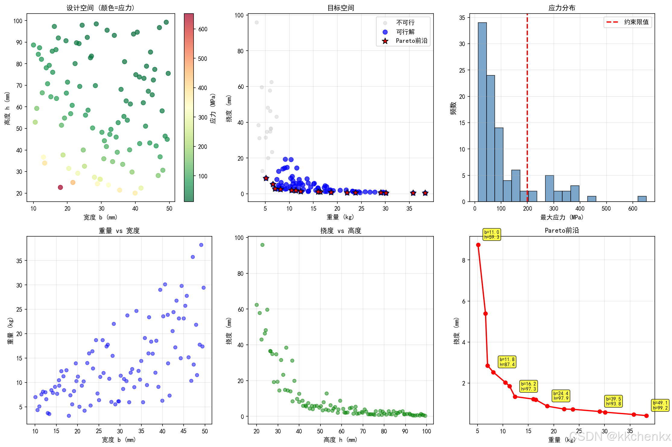
7.1 问题描述

考虑一个简化的工程优化问题：悬臂梁的截面尺寸优化。

设计变量：

$b$ ：梁宽度 (mm)
$h$ ：梁高度 (mm)

目标函数：

$f_1$ ：梁重量（最小化）
$f_2$ ：最大挠度（最小化）

约束条件：

最大应力 $σmax≤200\sigma_{max} \leq 200$ MPa
宽度范围： $\leq b \leq 50$ mm
高度范围： $\leq h \leq 100$ mm

7.2 Python实现：工程优化

import numpy as np
import matplotlib
matplotlib.use('Agg')
import matplotlib.pyplot as plt
from pyDOE2 import lhs
import os

plt.rcParams['font.sans-serif'] = ['SimHei', 'DejaVu Sans']
plt.rcParams['axes.unicode_minus'] = False

output_dir = os.path.join(os.path.dirname(__file__), 'output')
os.makedirs(output_dir, exist_ok=True)

# 悬臂梁问题参数
L = 1000  # 梁长度 (mm)
E = 200e3  # 弹性模量 (MPa)
F = 1000   # 端部载荷 (N)
rho = 7.85e-6  # 密度 (kg/mm³)

# 设计空间
bounds = np.array([[10, 50], [20, 100]])  # [b_min, b_max], [h_min, h_max]

def cantilever_analysis(x):
    """
    悬臂梁分析
    输入: x = [b, h] (mm)
    输出: [重量, 挠度, 最大应力]
    """
    b, h = x[:, 0], x[:, 1]
    
    # 截面惯性矩
    I = b * h**3 / 12
    
    # 截面面积
    A = b * h
    
    # 重量 (kg)
    weight = rho * A * L
    
    # 最大挠度 (mm)
    delta = F * L**3 / (3 * E * I)
    
    # 最大应力 (MPa) - 在固定端
    sigma_max = F * L * h / (2 * I)
    
    return np.column_stack([weight, delta, sigma_max])

# 生成样本数据
np.random.seed(42)
n_samples = 100
X_train = lhs(2, samples=n_samples)
X_train = bounds[:, 0] + X_train * (bounds[:, 1] - bounds[:, 0])
Y_train = cantilever_analysis(X_train)

# 提取目标函数和约束
weight = Y_train[:, 0]
deflection = Y_train[:, 1]
stress = Y_train[:, 2]

# 识别可行解和Pareto解
feasible_mask = stress <= 200
X_feasible = X_train[feasible_mask]
weight_feasible = weight[feasible_mask]
deflection_feasible = deflection[feasible_mask]

# 找到Pareto前沿（在可行解中）
def find_pareto_front(obj1, obj2):
    """找到Pareto前沿"""
    n = len(obj1)
    is_pareto = np.ones(n, dtype=bool)
    
    for i in range(n):
        for j in range(n):
            if i != j:
                if obj1[j] <= obj1[i] and obj2[j] <= obj2[i]:
                    if obj1[j] < obj1[i] or obj2[j] < obj2[i]:
                        is_pareto[i] = False
                        break
    
    return is_pareto

pareto_mask = find_pareto_front(weight_feasible, deflection_feasible)

# 可视化
fig, axes = plt.subplots(2, 3, figsize=(15, 10))

# 设计空间散点图
ax = axes[0, 0]
scatter = ax.scatter(X_train[:, 0], X_train[:, 1], c=stress, cmap='RdYlGn_r', s=50, alpha=0.7)
ax.contour(X_train[:, 0].reshape(10, 10), X_train[:, 1].reshape(10, 10), 
          stress.reshape(10, 10), levels=[200], colors='red', linewidths=2)
ax.set_xlabel('宽度 b (mm)', fontsize=10)
ax.set_ylabel('高度 h (mm)', fontsize=10)
ax.set_title('设计空间 (颜色=应力)', fontsize=11)
plt.colorbar(scatter, ax=ax, label='应力 (MPa)')

# 目标空间
ax = axes[0, 1]
ax.scatter(weight, deflection, c='lightgray', alpha=0.5, s=30, label='不可行')
ax.scatter(weight_feasible, deflection_feasible, c='blue', alpha=0.7, s=50, label='可行解')
ax.scatter(weight_feasible[pareto_mask], deflection_feasible[pareto_mask], 
          c='red', s=100, marker='*', edgecolors='black', label='Pareto前沿', zorder=5)
ax.set_xlabel('重量 (kg)', fontsize=10)
ax.set_ylabel('挠度 (mm)', fontsize=10)
ax.set_title('目标空间', fontsize=11)
ax.legend()
ax.grid(True, alpha=0.3)

# 应力分布
ax = axes[0, 2]
ax.hist(stress, bins=20, color='steelblue', alpha=0.7, edgecolor='black')
ax.axvline(x=200, color='red', linestyle='--', linewidth=2, label='约束限值')
ax.set_xlabel('最大应力 (MPa)', fontsize=10)
ax.set_ylabel('频数', fontsize=11)
ax.set_title('应力分布', fontsize=11)
ax.legend()
ax.grid(True, alpha=0.3)

# 重量vs宽度
ax = axes[1, 0]
ax.scatter(X_train[:, 0], weight, c='blue', alpha=0.5, s=30)
ax.set_xlabel('宽度 b (mm)', fontsize=10)
ax.set_ylabel('重量 (kg)', fontsize=10)
ax.set_title('重量 vs 宽度', fontsize=11)
ax.grid(True, alpha=0.3)

# 挠度vs高度
ax = axes[1, 1]
ax.scatter(X_train[:, 1], deflection, c='green', alpha=0.5, s=30)
ax.set_xlabel('高度 h (mm)', fontsize=10)
ax.set_ylabel('挠度 (mm)', fontsize=10)
ax.set_title('挠度 vs 高度', fontsize=11)
ax.grid(True, alpha=0.3)

# Pareto前沿详细图
ax = axes[1, 2]
pareto_weight = weight_feasible[pareto_mask]
pareto_deflection = deflection_feasible[pareto_mask]
pareto_b = X_feasible[pareto_mask, 0]
pareto_h = X_feasible[pareto_mask, 1]

# 按重量排序
sort_idx = np.argsort(pareto_weight)
ax.plot(pareto_weight[sort_idx], pareto_deflection[sort_idx], 'r-o', linewidth=2, markersize=6)
ax.set_xlabel('重量 (kg)', fontsize=10)
ax.set_ylabel('挠度 (mm)', fontsize=10)
ax.set_title('Pareto前沿', fontsize=11)
ax.grid(True, alpha=0.3)

# 添加设计参数标注
for i in range(0, len(pareto_weight), max(1, len(pareto_weight)//5)):
    idx = sort_idx[i]
    ax.annotate(f'b={pareto_b[idx]:.1f}\nh={pareto_h[idx]:.1f}', 
               xy=(pareto_weight[idx], pareto_deflection[idx]),
               xytext=(10, 10), textcoords='offset points', fontsize=8,
               bbox=dict(boxstyle='round,pad=0.3', facecolor='yellow', alpha=0.7))

plt.tight_layout()
plt.savefig(os.path.join(output_dir, 'case6_engineering_design.png'), dpi=150, bbox_inches='tight')
plt.close()

# 打印Pareto解
print("\nPareto最优解:")
print("=" * 60)
print(f"{'重量(kg)':<12}{'挠度(mm)':<12}{'应力(MPa)':<12}{'b(mm)':<10}{'h(mm)':<10}")
print("=" * 60)
for i in sort_idx:
    print(f"{pareto_weight[i]:<12.3f}{pareto_deflection[i]:<12.3f}"
          f"{stress[feasible_mask][i]:<12.1f}{pareto_b[i]:<10.1f}{pareto_h[i]:<10.1f}")
print("=" * 60)

print("✓ 工程优化案例完成")

8. 结论与展望

8.1 代理模型技术的核心优势

代理模型技术为解决昂贵黑箱函数的优化问题提供了有效途径，其核心优势体现在以下几个方面：

计算效率的显著提升：代理模型将优化搜索从昂贵的仿真转移到廉价的近似模型，计算成本降低数个数量级。以本教程中的悬臂梁优化为例，单次有限元分析可能需要数分钟，而代理模型评估仅需毫秒级时间。对于需要数千次评估的优化过程，这种效率提升是革命性的。

全局搜索能力：代理模型具有良好的平滑性，便于应用遗传算法、粒子群优化等全局优化算法，有效避免陷入局部最优解。相比传统的基于梯度的局部优化方法，代理模型辅助的全局优化能够发现更优的设计方案。

不确定性量化能力：Kriging等概率代理模型不仅提供预测均值，还能给出预测方差，为基于信息的自适应采样提供了理论基础。通过期望改进（EI）等采集函数，可以智能地选择下一个评估点，实现探索与利用的平衡。

多目标优化的自然支持：代理模型可以方便地扩展到多目标优化问题，通过构建每个目标函数的代理模型，结合NSGA-II等进化算法，高效地搜索Pareto最优解集，为工程决策提供丰富的选择。

并行化潜力：代理模型的训练和评估过程天然适合并行计算，可以充分利用现代高性能计算资源，进一步加速优化过程。

8.2 代理模型技术的局限性

尽管代理模型技术具有显著优势，但在实际应用中也存在一些局限性：

维度灾难问题：随着设计变量维度的增加，所需样本点数量呈指数增长。对于高维问题（维度>20），传统的代理模型方法面临"维度灾难"，建模精度难以保证。

非平稳性问题：对于高度非线性的黑箱函数，单一代理模型可能难以在整个设计空间上保持高精度。此时需要采用自适应采样或多保真度建模策略。

约束处理挑战：含约束的优化问题需要同时构建目标函数和约束函数的代理模型，增加了建模复杂度。此外，代理模型预测的约束违反可能存在误差，导致优化结果不可行。

模型验证需求：代理模型的精度依赖于训练样本的质量和数量，需要通过交叉验证等方法评估模型可靠性，增加了计算成本。

8.3 前沿发展方向

代理模型技术正在与多个前沿领域深度融合，展现出广阔的发展前景：

深度学习代理模型：神经网络，特别是深度神经网络和物理信息神经网络（PINN），为高维复杂问题的代理建模提供了新工具。深度学习方法能够自动学习特征表示，在处理图像、流场等复杂数据时展现出优势。

多保真度建模：结合高保真度和低保真度仿真数据，构建多保真度代理模型，在保持精度的同时进一步降低计算成本。协同Kriging（Co-Kriging）等方法能够有效融合不同 fidelity 的数据源。

自适应采样与主动学习：基于贝叶斯优化的自适应采样策略，通过最大化信息增益选择下一个评估点，实现样本的高效利用。这一方向在超参数优化、实验设计等领域有广泛应用。

多目标贝叶斯优化：将贝叶斯优化扩展到多目标场景，通过构建多目标采集函数，直接搜索Pareto前沿，避免显式构建所有目标函数的代理模型。

物理信息融合：将物理约束嵌入代理模型，如物理信息Kriging、物理信息神经网络等，提高模型的外推能力和物理一致性。

不确定性量化与鲁棒优化：利用代理模型的预测不确定性进行鲁棒优化和可靠性分析，确保设计方案在不确定性条件下的性能稳定性。

8.4 工程应用建议

基于本教程的理论分析和案例实践，对工程应用提出以下建议：

采样策略选择：对于低维问题（维度<5），推荐使用全因子或中心复合设计；对于中高维问题，拉丁超立方采样是首选；对于高维问题，可以考虑稀疏网格或自适应采样方法。

代理模型选择：

对于平滑、低非线性的响应，响应面方法（RSM）简单高效
对于中等非线性问题，Kriging模型能够提供良好的插值精度和不确定性估计
对于高度非线性或高维问题，可以考虑径向基函数（RBF）或神经网络

模型验证：必须采用交叉验证或独立测试集评估代理模型精度，确保R²>0.9且RMSE在可接受范围内。对于关键设计区域，应增加样本点密度。

优化策略：推荐采用序列优化策略，初始阶段使用较少样本点构建粗糙代理模型，逐步添加样本点 refine 模型，直至收敛。

约束处理：对于含约束的优化问题，建议构建约束函数的代理模型，并在优化过程中考虑代理模型的预测不确定性，避免违反约束。

多目标处理：对于多目标优化，推荐使用NSGA-II等进化算法搜索Pareto前沿，结合决策者的偏好信息选择最终设计方案。

8.5 总结

代理模型与优化技术是现代工程设计中不可或缺的工具。本教程系统介绍了代理模型的理论基础、核心方法和工程应用，通过Python实现了六个典型案例，涵盖了试验设计、响应面方法、Kriging模型、序列优化、多目标优化和工程应用等核心内容。

通过本教程的学习，读者应该能够：

理解代理模型的基本原理和数学基础
掌握试验设计方法，合理选择样本点
构建和验证响应面模型与Kriging模型
实现代理模型辅助的优化策略
应用多目标优化算法解决实际工程问题
评估代理模型的精度并选择合适的建模方法

代理模型技术仍在快速发展中，与机器学习、不确定性量化等领域的交叉融合将带来更多创新方法。希望本教程能够为读者在这一领域的深入研究和工程实践奠定坚实基础。

参考文献

[1] Box G E P, Wilson K B. On the experimental attainment of optimum conditions[J]. Journal of the Royal Statistical Society: Series B (Methodological), 1951, 13(1): 1-38.

[2] Sacks J, Welch W J, Mitchell T J, et al. Design and analysis of computer experiments[J]. Statistical Science, 1989, 4(4): 409-423.

[3] Jones D R, Schonlau M, Welch W J. Efficient global optimization of expensive black-box functions[J]. Journal of Global Optimization, 1998, 13(4): 455-492.

[4] Deb K, Pratap A, Agarwal S, et al. A fast and elitist multiobjective genetic algorithm: NSGA-II[J]. IEEE Transactions on Evolutionary Computation, 2002, 6(2): 182-197.

[5] Forrester A I J, Sobester A, Keane A J. Engineering design via surrogate modelling: a practical guide[M]. John Wiley & Sons, 2008.

[6] Queipo N V, Haftka R T, Shyy W, et al. Surrogate-based analysis and optimization[J]. Progress in Aerospace Sciences, 2005, 41(1): 1-28.

[7] Simpson T W, Peplinski J D, Koch P N, et al. Metamodels for computer-based engineering design: survey and recommendations[J]. Engineering with Computers, 2001, 17(2): 129-150.

[8] Kleijnen J P C. Kriging metamodeling in simulation: a review[J]. European Journal of Operational Research, 2009, 192(3): 707-716.

[9] Viana F A C, Simpson T W, Balabanov V, et al. Metamodeling in multidisciplinary design optimization: how far have we really come?[J]. AIAA Journal, 2014, 52(4): 670-690.

[10] Rasmussen C E, Williams C K I. Gaussian processes for machine learning[M]. MIT Press, 2006.

[11] Lophaven S N, Nielsen H B, Søndergaard J. DACE: A Matlab Kriging toolbox[R]. Technical University of Denmark, 2002.

[12] Gorissen D, Couckuyt I, Demeester P, et al. A surrogate modeling and adaptive sampling toolbox for computer based design[J]. Journal of Machine Learning Research, 2010, 11: 2051-2055.

[13] 韩忠华. Kriging模型及代理优化算法研究进展[J]. 航空学报, 2016, 37(11): 3197-3225.

[14] 张科, 李道奎. 基于代理模型的优化设计方法研究进展[J]. 机械工程学报, 2015, 51(13): 91-102.

[15] 王振峰, 范子杰. 基于Kriging代理模型的多学科设计优化方法[J]. 机械工程学报, 2013, 49(19): 115-122.

[16] McKay M D, Beckman R J, Conover W J. A comparison of three methods for selecting values of input variables in the analysis of output from a computer code[J]. Technometrics, 1979, 21(2): 239-245.

[17] Santner T J, Williams B J, Notz W I. The design and analysis of computer experiments[M]. Springer, 2003.

[18] Fang K T, Li R, Sudjianto A. Design and modeling for computer experiments[M]. Chapman and Hall/CRC, 2005.

[19] Knowles J. ParEGO: a hybrid algorithm with on-line landscape approximation for expensive multiobjective optimization problems[J]. IEEE Transactions on Evolutionary Computation, 2006, 10(1): 50-66.

[20] Ponweiser W, Wagner T, Biermann D, et al. Multiobjective optimization on a limited budget of evaluations using model-assisted S-metric selection[C]. International Conference on Parallel Problem Solving from Nature. Springer, 2008: 784-794.

附录：Python程序完整代码

本教程所有案例的完整Python代码如下，可直接运行：

"""
主题062：代理模型与优化
完整仿真程序
"""

import numpy as np
import matplotlib
matplotlib.use('Agg')
import matplotlib.pyplot as plt
from scipy.optimize import minimize
import os

plt.rcParams['font.sans-serif'] = ['SimHei', 'DejaVu Sans']
plt.rcParams['axes.unicode_minus'] = False

output_dir = os.path.join(os.path.dirname(__file__), 'output')
os.makedirs(output_dir, exist_ok=True)

print("="*60)
print("主题062：代理模型与优化")
print("="*60)

# ==================== 案例1: 试验设计方法 ====================
print("\n【案例1: 试验设计方法对比】")

def lhs_sampling(n_samples, n_dim):
    """拉丁超立方采样"""
    samples = np.zeros((n_samples, n_dim))
    for i in range(n_dim):
        perm = np.random.permutation(n_samples)
        samples[:, i] = (perm + np.random.rand(n_samples)) / n_samples
    return samples

np.random.seed(42)
d = 2
n_samples = 20

# 随机采样
random_samples = np.random.rand(n_samples, d)

# LHS采样
lhs_samples = lhs_sampling(n_samples, d)

# 网格采样
n_grid = int(np.sqrt(n_samples))
x_grid = np.linspace(0, 1, n_grid)
y_grid = np.linspace(0, 1, n_grid)
X_grid, Y_grid = np.meshgrid(x_grid, y_grid)
grid_samples = np.column_stack([X_grid.flatten(), Y_grid.flatten()])

# 可视化
fig, axes = plt.subplots(1, 3, figsize=(15, 5))

axes[0].scatter(random_samples[:, 0], random_samples[:, 1], c='blue', s=50, alpha=0.7)
axes[0].set_xlabel('设计变量 x₁', fontsize=11)
axes[0].set_ylabel('设计变量 x₂', fontsize=11)
axes[0].set_title('随机采样', fontsize=12)
axes[0].grid(True, alpha=0.3)
axes[0].set_xlim(0, 1)
axes[0].set_ylim(0, 1)

axes[1].scatter(lhs_samples[:, 0], lhs_samples[:, 1], c='red', s=50, alpha=0.7)
axes[1].set_xlabel('设计变量 x₁', fontsize=11)
axes[1].set_ylabel('设计变量 x₂', fontsize=11)
axes[1].set_title('拉丁超立方采样 (LHS)', fontsize=12)
axes[1].grid(True, alpha=0.3)
axes[1].set_xlim(0, 1)
axes[1].set_ylim(0, 1)

axes[2].scatter(grid_samples[:, 0], grid_samples[:, 1], c='green', s=50, alpha=0.7)
axes[2].set_xlabel('设计变量 x₁', fontsize=11)
axes[2].set_ylabel('设计变量 x₂', fontsize=11)
axes[2].set_title('网格采样', fontsize=12)
axes[2].grid(True, alpha=0.3)
axes[2].set_xlim(0, 1)
axes[2].set_ylim(0, 1)

plt.tight_layout()
plt.savefig(os.path.join(output_dir, 'case1_sampling_methods.png'), dpi=150, bbox_inches='tight')
plt.close()
print("✓ 试验设计方法对比完成")

# ==================== 案例2: 响应面方法 ====================
print("\n【案例2: 响应面方法】")

def branin(x):
    """Branin测试函数"""
    x1, x2 = x[:, 0], x[:, 1]
    a = 1
    b = 5.1 / (4 * np.pi**2)
    c = 5 / np.pi
    r = 6
    s = 10
    t = 1 / (8 * np.pi)
    return a * (x2 - b*x1**2 + c*x1 - r)**2 + s*(1-t)*np.cos(x1) + s

bounds = np.array([[-5, 10], [0, 15]])

# 生成训练样本
np.random.seed(42)
n_train = 30
X_train = lhs_sampling(n_train, 2)
X_train = bounds[:, 0] + X_train * (bounds[:, 1] - bounds[:, 0])
y_train = branin(X_train)

# 生成测试样本
n_test = 1000
X_test = np.random.rand(n_test, 2)
X_test = bounds[:, 0] + X_test * (bounds[:, 1] - bounds[:, 0])
y_test = branin(X_test)

# 多项式特征生成
def polynomial_features(X, degree):
    """生成多项式特征"""
    n_samples, n_features = X.shape
    if degree == 1:
        features = np.column_stack([np.ones(n_samples), X])
    elif degree == 2:
        features = [np.ones(n_samples), X[:, 0], X[:, 1]]
        features.extend([X[:, 0]**2, X[:, 1]**2, X[:, 0]*X[:, 1]])
        features = np.column_stack(features)
    return features

# 线性模型
X_train_linear = polynomial_features(X_train, 1)
X_test_linear = polynomial_features(X_test, 1)
beta_linear = np.linalg.lstsq(X_train_linear, y_train, rcond=None)[0]
y_pred_linear = X_test_linear @ beta_linear

# 二次模型
X_train_quad = polynomial_features(X_train, 2)
X_test_quad = polynomial_features(X_test, 2)
beta_quad = np.linalg.lstsq(X_train_quad, y_train, rcond=None)[0]
y_pred_quad = X_test_quad @ beta_quad

# 评估
r2_linear = 1 - np.sum((y_test - y_pred_linear)**2) / np.sum((y_test - np.mean(y_test))**2)
r2_quad = 1 - np.sum((y_test - y_pred_quad)**2) / np.sum((y_test - np.mean(y_test))**2)
rmse_linear = np.sqrt(np.mean((y_test - y_pred_linear)**2))
rmse_quad = np.sqrt(np.mean((y_test - y_pred_quad)**2))

print(f"线性模型: R² = {r2_linear:.4f}, RMSE = {rmse_linear:.4f}")
print(f"二次模型: R² = {r2_quad:.4f}, RMSE = {rmse_quad:.4f}")

# 可视化
fig, axes = plt.subplots(2, 3, figsize=(15, 10))

x1_grid = np.linspace(bounds[0, 0], bounds[0, 1], 100)
x2_grid = np.linspace(bounds[1, 0], bounds[1, 1], 100)
X1_grid, X2_grid = np.meshgrid(x1_grid, x2_grid)
X_grid = np.column_stack([X1_grid.flatten(), X2_grid.flatten()])
y_grid = branin(X_grid).reshape(X1_grid.shape)

# 真实函数
ax = axes[0, 0]
im = ax.contourf(X1_grid, X2_grid, y_grid, levels=20, cmap='viridis')
ax.scatter(X_train[:, 0], X_train[:, 1], c='red', s=30, edgecolors='white')
ax.set_xlabel('x₁', fontsize=10)
ax.set_ylabel('x₂', fontsize=10)
ax.set_title('真实函数 (Branin)', fontsize=11)
plt.colorbar(im, ax=ax)

# 线性模型
y_linear_grid = polynomial_features(X_grid, 1) @ beta_linear
y_linear_grid = y_linear_grid.reshape(X1_grid.shape)
ax = axes[0, 1]
im = ax.contourf(X1_grid, X2_grid, y_linear_grid, levels=20, cmap='viridis')
ax.set_xlabel('x₁', fontsize=10)
ax.set_ylabel('x₂', fontsize=10)
ax.set_title(f'线性RSM (R²={r2_linear:.3f})', fontsize=11)
plt.colorbar(im, ax=ax)

# 二次模型
y_quad_grid = polynomial_features(X_grid, 2) @ beta_quad
y_quad_grid = y_quad_grid.reshape(X1_grid.shape)
ax = axes[0, 2]
im = ax.contourf(X1_grid, X2_grid, y_quad_grid, levels=20, cmap='viridis')
ax.set_xlabel('x₁', fontsize=10)
ax.set_ylabel('x₂', fontsize=10)
ax.set_title(f'二次RSM (R²={r2_quad:.3f})', fontsize=11)
plt.colorbar(im, ax=ax)

# 误差图
ax = axes[1, 0]
im = ax.contourf(X1_grid, X2_grid, np.abs(y_grid - y_linear_grid), levels=20, cmap='hot')
ax.set_xlabel('x₁', fontsize=10)
ax.set_ylabel('x₂', fontsize=10)
ax.set_title('线性模型绝对误差', fontsize=11)
plt.colorbar(im, ax=ax)

ax = axes[1, 1]
im = ax.contourf(X1_grid, X2_grid, np.abs(y_grid - y_quad_grid), levels=20, cmap='hot')
ax.set_xlabel('x₁', fontsize=10)
ax.set_ylabel('x₂', fontsize=10)
ax.set_title('二次模型绝对误差', fontsize=11)
plt.colorbar(im, ax=ax)

# 预测vs真实
ax = axes[1, 2]
ax.scatter(y_test, y_pred_linear, c='blue', alpha=0.5, label='线性模型', s=20)
ax.scatter(y_test, y_pred_quad, c='red', alpha=0.5, label='二次模型', s=20)
ax.plot([y_test.min(), y_test.max()], [y_test.min(), y_test.max()], 'k--', lw=2)
ax.set_xlabel('真实值', fontsize=10)
ax.set_ylabel('预测值', fontsize=10)
ax.set_title('预测值 vs 真实值', fontsize=11)
ax.legend()
ax.grid(True, alpha=0.3)

plt.tight_layout()
plt.savefig(os.path.join(output_dir, 'case2_response_surface.png'), dpi=150, bbox_inches='tight')
plt.close()
print("✓ 响应面方法完成")

# ==================== 案例3: Kriging模型 ====================
print("\n【案例3: Kriging模型】")

def hartmann3(x):
    """Hartmann 3D测试函数"""
    alpha = np.array([1.0, 1.2, 3.0, 3.2])
    A = np.array([[3.0, 10, 30],
                  [0.1, 10, 35],
                  [3.0, 10, 30],
                  [0.1, 10, 35]])
    P = 1e-4 * np.array([[3689, 1170, 2673],
                         [4699, 4387, 7470],
                         [1091, 8732, 5547],
                         [381, 5743, 8828]])
    
    y = 0
    for i in range(4):
        inner = 0
        for j in range(3):
            inner += A[i, j] * (x[:, j] - P[i, j])**2
        y += alpha[i] * np.exp(-inner)
    return -y

def gaussian_correlation(X1, X2, theta):
    """高斯相关函数"""
    n1, d = X1.shape
    n2 = X2.shape[0]
    R = np.zeros((n1, n2))
    for i in range(n1):
        for j in range(n2):
            diff = X1[i] - X2[j]
            R[i, j] = np.exp(-np.sum(theta * diff**2))
    return R

class KrigingModel:
    """Kriging模型类"""
    def __init__(self, theta0=None):
        self.theta = theta0
        self.X_train = None
        self.y_train = None
        self.mu = None
        self.sigma2 = None
        self.R_inv = None
        
    def fit(self, X, y):
        self.X_train = X.copy()
        self.y_train = y.copy()
        n, d = X.shape
        
        if self.theta is None:
            def neg_log_likelihood(theta):
                R = gaussian_correlation(X, X, theta) + 1e-10 * np.eye(n)
                try:
                    R_inv = np.linalg.inv(R)
                except:
                    return 1e10
                ones = np.ones(n)
                mu = (ones @ R_inv @ y) / (ones @ R_inv @ ones)
                sigma2 = ((y - mu) @ R_inv @ (y - mu)) / n
                if sigma2 <= 0:
                    return 1e10
                return n * np.log(sigma2) + np.log(np.linalg.det(R))
            
            bounds = [(1e-3, 10) for _ in range(d)]
            result = minimize(neg_log_likelihood, np.ones(d), method='L-BFGS-B', bounds=bounds)
            self.theta = result.x
        
        R = gaussian_correlation(X, X, self.theta) + 1e-10 * np.eye(n)
        self.R_inv = np.linalg.inv(R)
        ones = np.ones(n)
        self.mu = (ones @ self.R_inv @ y) / (ones @ self.R_inv @ ones)
        self.sigma2 = ((y - self.mu) @ self.R_inv @ (y - self.mu)) / n
        
    def predict(self, X, return_std=False):
        n_train = self.X_train.shape[0]
        r = gaussian_correlation(X, self.X_train, self.theta)
        y_pred = self.mu + r @ self.R_inv @ (self.y_train - self.mu)
        
        if return_std:
            ones = np.ones(n_train)
            u = ones @ self.R_inv @ r.T
            r_self = np.array([gaussian_correlation(X[i:i+1], X[i:i+1], self.theta)[0, 0] 
                              for i in range(X.shape[0])])
            sigma2_pred = self.sigma2 * (1 - np.sum(r * (self.R_inv @ r.T).T, axis=1) + 
                                      (1 - u)**2 / (ones @ self.R_inv @ ones))
            sigma2_pred = np.maximum(sigma2_pred, 0)
            return y_pred, np.sqrt(sigma2_pred)
        return y_pred

# 生成样本
np.random.seed(42)
n_train = 50
X_train = lhs_sampling(n_train, 3)
y_train = hartmann3(X_train)

n_test = 200
X_test = np.random.rand(n_test, 3)
y_test = hartmann3(X_test)

# 训练Kriging模型
kriging = KrigingModel()
kriging.fit(X_train, y_train)
y_pred_kriging, y_std = kriging.predict(X_test, return_std=True)

# 评估
r2_kriging = 1 - np.sum((y_test - y_pred_kriging)**2) / np.sum((y_test - np.mean(y_test))**2)
rmse_kriging = np.sqrt(np.mean((y_test - y_pred_kriging)**2))

print(f"Kriging模型: R² = {r2_kriging:.4f}, RMSE = {rmse_kriging:.4f}")
print(f"估计的超参数 theta: {kriging.theta}")

# 可视化
fig, axes = plt.subplots(2, 2, figsize=(12, 10))

# 预测vs真实
ax = axes[0, 0]
ax.scatter(y_test, y_pred_kriging, c='blue', alpha=0.5, s=30)
ax.plot([y_test.min(), y_test.max()], [y_test.min(), y_test.max()], 'r--', lw=2)
ax.set_xlabel('真实值', fontsize=11)
ax.set_ylabel('预测值', fontsize=11)
ax.set_title(f'Kriging预测 (R²={r2_kriging:.3f})', fontsize=12)
ax.grid(True, alpha=0.3)

# 预测标准差
ax = axes[0, 1]
ax.scatter(y_test, y_std, c='green', alpha=0.5, s=30)
ax.set_xlabel('真实值', fontsize=11)
ax.set_ylabel('预测标准差', fontsize=11)
ax.set_title('预测不确定性', fontsize=12)
ax.grid(True, alpha=0.3)

# 残差分布
ax = axes[1, 0]
residuals = y_test - y_pred_kriging
ax.hist(residuals, bins=30, color='steelblue', alpha=0.7, edgecolor='black')
ax.axvline(x=0, color='red', linestyle='--', linewidth=2)
ax.set_xlabel('残差', fontsize=11)
ax.set_ylabel('频数', fontsize=11)
ax.set_title('残差分布', fontsize=12)
ax.grid(True, alpha=0.3)

# 误差vs不确定性
ax = axes[1, 1]
ax.scatter(y_std, np.abs(residuals), c='purple', alpha=0.5, s=30)
ax.set_xlabel('预测标准差', fontsize=11)
ax.set_ylabel('绝对误差', fontsize=11)
ax.set_title('误差 vs 不确定性', fontsize=12)
ax.grid(True, alpha=0.3)

plt.tight_layout()
plt.savefig(os.path.join(output_dir, 'case3_kriging.png'), dpi=150, bbox_inches='tight')
plt.close()
print("✓ Kriging模型完成")

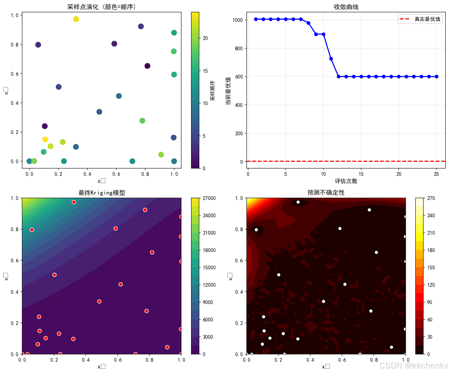
# ==================== 案例4: 序列优化 ====================
print("\n【案例4: 序列优化与自适应采样】")

def expensive_function(x):
    """模拟昂贵函数 - Goldstein-Price函数"""
    x1, x2 = x[:, 0], x[:, 1]
    term1 = 1 + (x1 + x2 + 1)**2 * (19 - 14*x1 + 3*x1**2 - 14*x2 + 6*x1*x2 + 3*x2**2)
    term2 = 30 + (2*x1 - 3*x2)**2 * (18 - 32*x1 + 12*x1**2 + 48*x2 - 36*x1*x2 + 27*x2**2)
    return term1 * term2

# 初始采样
np.random.seed(42)
X_train = lhs_sampling(10, 2)
y_train = expensive_function(X_train)

# 序列优化
n_iterations = 15
X_all = X_train.copy()
y_all = y_train.copy()

for iteration in range(n_iterations):
    # 构建Kriging模型
    kriging = KrigingModel()
    kriging.fit(X_all, y_all)
    
    # 期望改进函数
    def neg_expected_improvement(x):
        x = x.reshape(1, -1)
        y_pred, y_std = kriging.predict(x, return_std=True)
        y_min = np.min(y_all)
        
        if y_std[0] < 1e-10:
            return 0
        
        z = (y_min - y_pred[0]) / y_std[0]
        ei = (y_min - y_pred[0]) * (0.5 * (1 + np.sign(z))) + y_std[0] * np.exp(-z**2/2) / np.sqrt(2*np.pi)
        return -ei
    
    # 优化EI找到下一个采样点
    best_ei = -np.inf
    best_x = None
    for _ in range(50):
        x0 = np.random.rand(2)
        result = minimize(neg_expected_improvement, x0, method='L-BFGS-B', 
                         bounds=[(0, 1), (0, 1)])
        if -result.fun > best_ei:
            best_ei = -result.fun
            best_x = result.x
    
    # 添加新样本
    y_new = expensive_function(best_x.reshape(1, -1))
    X_all = np.vstack([X_all, best_x])
    y_all = np.append(y_all, y_new)
    
    if iteration % 5 == 0:
        print(f"迭代 {iteration}: 当前最优值 = {np.min(y_all):.4f}, EI = {best_ei:.4f}")

print(f"最终最优值: {np.min(y_all):.4f} (真实最优 ≈ 3.0)")

# 可视化
fig, axes = plt.subplots(2, 2, figsize=(12, 10))

# 采样点演化
ax = axes[0, 0]
scatter = ax.scatter(X_all[:, 0], X_all[:, 1], c=range(len(X_all)), cmap='viridis', s=100)
ax.set_xlabel('x₁', fontsize=11)
ax.set_ylabel('x₂', fontsize=11)
ax.set_title('采样点演化 (颜色=顺序)', fontsize=12)
plt.colorbar(scatter, ax=ax, label='采样顺序')

# 目标函数值收敛
ax = axes[0, 1]
y_best_history = [np.min(y_all[:i+1]) for i in range(len(y_all))]
ax.plot(range(1, len(y_all)+1), y_best_history, 'b-o', linewidth=2, markersize=6)
ax.axhline(y=3.0, color='red', linestyle='--', linewidth=2, label='真实最优值')
ax.set_xlabel('评估次数', fontsize=11)
ax.set_ylabel('当前最优值', fontsize=11)
ax.set_title('收敛曲线', fontsize=12)
ax.legend()
ax.grid(True, alpha=0.3)

# 最终Kriging模型
kriging_final = KrigingModel()
kriging_final.fit(X_all, y_all)

x1_grid = np.linspace(0, 1, 50)
x2_grid = np.linspace(0, 1, 50)
X1_grid, X2_grid = np.meshgrid(x1_grid, x2_grid)
X_grid = np.column_stack([X1_grid.flatten(), X2_grid.flatten()])
y_pred_grid = kriging_final.predict(X_grid).reshape(X1_grid.shape)

ax = axes[1, 0]
im = ax.contourf(X1_grid, X2_grid, y_pred_grid, levels=20, cmap='viridis')
ax.scatter(X_all[:, 0], X_all[:, 1], c='red', s=50, edgecolors='white')
ax.set_xlabel('x₁', fontsize=11)
ax.set_ylabel('x₂', fontsize=11)
ax.set_title('最终Kriging模型', fontsize=12)
plt.colorbar(im, ax=ax)

# 预测不确定性
_, y_std_grid = kriging_final.predict(X_grid, return_std=True)
y_std_grid = y_std_grid.reshape(X1_grid.shape)

ax = axes[1, 1]
im = ax.contourf(X1_grid, X2_grid, y_std_grid, levels=20, cmap='hot')
ax.scatter(X_all[:, 0], X_all[:, 1], c='white', s=50, edgecolors='black')
ax.set_xlabel('x₁', fontsize=11)
ax.set_ylabel('x₂', fontsize=11)
ax.set_title('预测不确定性', fontsize=12)
plt.colorbar(im, ax=ax)

plt.tight_layout()
plt.savefig(os.path.join(output_dir, 'case4_sequential_optimization.png'), dpi=150, bbox_inches='tight')
plt.close()
print("✓ 序列优化完成")

# ==================== 案例5: 多目标优化 ====================
print("\n【案例5: 多目标优化 (NSGA-II)】")

def zdt1(x):
    """ZDT1测试函数"""
    f1 = x[:, 0]
    g = 1 + 9 * np.sum(x[:, 1:], axis=1) / (x.shape[1] - 1)
    h = 1 - np.sqrt(f1 / g)
    f2 = g * h
    return np.column_stack([f1, f2])

class NSGA2:
    """NSGA-II算法实现"""
    def __init__(self, n_obj=2, bounds=np.array([[0, 1], [0, 1], [0, 1]]), 
                 pop_size=100, n_gen=200):
        self.n_obj = n_obj
        self.n_var = bounds.shape[0]
        self.bounds = bounds
        self.pop_size = pop_size
        self.n_gen = n_gen
        
    def initialize(self):
        return np.random.rand(self.pop_size, self.n_var) * \
               (self.bounds[:, 1] - self.bounds[:, 0]) + self.bounds[:, 0]
    
    def evaluate(self, pop):
        return zdt1(pop)
    
    def non_dominated_sort(self, objectives):
        n = objectives.shape[0]
        domination_count = np.zeros(n)
        dominated_solutions = [[] for _ in range(n)]
        fronts = [[]]
        
        for i in range(n):
            for j in range(i+1, n):
                if self.dominates(objectives[i], objectives[j]):
                    dominated_solutions[i].append(j)
                    domination_count[j] += 1
                elif self.dominates(objectives[j], objectives[i]):
                    dominated_solutions[j].append(i)
                    domination_count[i] += 1
            if domination_count[i] == 0:
                fronts[0].append(i)
        
        i = 0
        while len(fronts[i]) > 0:
            next_front = []
            for p in fronts[i]:
                for q in dominated_solutions[p]:
                    domination_count[q] -= 1
                    if domination_count[q] == 0:
                        next_front.append(q)
            i += 1
            fronts.append(next_front)
        fronts.pop()
        return fronts
    
    def dominates(self, obj1, obj2):
        return np.all(obj1 <= obj2) and np.any(obj1 < obj2)
    
    def crowding_distance(self, objectives, front):
        if len(front) <= 2:
            return np.full(len(front), np.inf)
        distances = np.zeros(len(front))
        for m in range(self.n_obj):
            sorted_indices = np.argsort(objectives[front, m])
            distances[sorted_indices[0]] = np.inf
            distances[sorted_indices[-1]] = np.inf
            f_max = objectives[front[sorted_indices[-1]], m]
            f_min = objectives[front[sorted_indices[0]], m]
            if f_max > f_min:
                for i in range(1, len(front)-1):
                    distances[sorted_indices[i]] += (
                        objectives[front[sorted_indices[i+1]], m] - 
                        objectives[front[sorted_indices[i-1]], m]
                    ) / (f_max - f_min)
        return distances
    
    def tournament_selection(self, pop, objectives, fronts):
        selected = []
        for _ in range(self.pop_size):
            i, j = np.random.choice(len(pop), 2, replace=False)
            rank_i = next(r for r, front in enumerate(fronts) if i in front)
            rank_j = next(r for r, front in enumerate(fronts) if j in front)
            if rank_i < rank_j:
                selected.append(i)
            elif rank_j < rank_i:
                selected.append(j)
            else:
                front_idx = [k for k, front in enumerate(fronts) if i in front][0]
                front = fronts[front_idx]
                distances = self.crowding_distance(objectives, front)
                idx_in_front_i = front.index(i)
                idx_in_front_j = front.index(j)
                if distances[idx_in_front_i] > distances[idx_in_front_j]:
                    selected.append(i)
                else:
                    selected.append(j)
        return pop[selected]
    
    def crossover(self, parent1, parent2):
        eta = 20
        u = np.random.rand(self.n_var)
        beta = np.where(u <= 0.5, (2*u)**(1/(eta+1)), (2*(1-u))**(-1/(eta+1)))
        child1 = 0.5 * ((1+beta)*parent1 + (1-beta)*parent2)
        child2 = 0.5 * ((1-beta)*parent1 + (1+beta)*parent2)
        return child1, child2
    
    def mutate(self, individual):
        eta_m = 20
        prob = 1.0 / self.n_var
        for i in range(self.n_var):
            if np.random.rand() < prob:
                u = np.random.rand()
                delta = np.where(u <= 0.5, 
                               (2*u)**(1/(eta_m+1)) - 1,
                               1 - (2*(1-u))**(1/(eta_m+1)))
                individual[i] += delta * (self.bounds[i, 1] - self.bounds[i, 0])
        return np.clip(individual, self.bounds[:, 0], self.bounds[:, 1])
    
    def run(self):
        pop = self.initialize()
        objectives = self.evaluate(pop)
        
        for generation in range(self.n_gen):
            fronts = self.non_dominated_sort(objectives)
            mating_pool = self.tournament_selection(pop, objectives, fronts)
            
            offspring = []
            for i in range(0, self.pop_size, 2):
                parent1 = mating_pool[i]
                parent2 = mating_pool[(i+1) % self.pop_size]
                child1, child2 = self.crossover(parent1, parent2)
                offspring.append(self.mutate(child1))
                offspring.append(self.mutate(child2))
            
            offspring = np.array(offspring[:self.pop_size])
            offspring_obj = self.evaluate(offspring)
            
            combined_pop = np.vstack([pop, offspring])
            combined_obj = np.vstack([objectives, offspring_obj])
            fronts = self.non_dominated_sort(combined_obj)
            
            new_pop = []
            new_obj = []
            for front in fronts:
                if len(new_pop) + len(front) <= self.pop_size:
                    new_pop.extend(combined_pop[front])
                    new_obj.extend(combined_obj[front])
                else:
                    distances = self.crowding_distance(combined_obj, front)
                    sorted_idx = np.argsort(distances)[::-1]
                    remaining = self.pop_size - len(new_pop)
                    for i in range(remaining):
                        new_pop.append(combined_pop[front[sorted_idx[i]]])
                        new_obj.append(combined_obj[front[sorted_idx[i]]])
                    break
            
            pop = np.array(new_pop)
            objectives = np.array(new_obj)
            
            if generation % 50 == 0:
                print(f"Generation {generation}: {len(fronts[0])} Pareto solutions")
        
        return pop, objectives

print("运行NSGA-II多目标优化...")
nsga2 = NSGA2(n_obj=2, bounds=np.array([[0, 1], [0, 1], [0, 1]]), pop_size=100, n_gen=200)
pop_final, obj_final = nsga2.run()

fronts = nsga2.non_dominated_sort(obj_final)
pareto_front = obj_final[fronts[0]]
print(f"找到 {len(pareto_front)} 个Pareto最优解")

# 可视化
fig, axes = plt.subplots(2, 2, figsize=(12, 10))

ax = axes[0, 0]
ax.scatter(obj_final[:, 0], obj_final[:, 1], c='lightblue', alpha=0.5, s=20, label='所有解')
ax.scatter(pareto_front[:, 0], pareto_front[:, 1], c='red', s=50, edgecolors='black', 
          label='Pareto前沿', zorder=5)
ax.set_xlabel('f₁', fontsize=11)
ax.set_ylabel('f₂', fontsize=11)
ax.set_title('NSGA-II优化结果 (ZDT1)', fontsize=12)
ax.legend()
ax.grid(True, alpha=0.3)

ax = axes[0, 1]
ax.scatter(pop_final[:, 0], pop_final[:, 1], c='blue', alpha=0.5, s=20)
ax.set_xlabel('x₁', fontsize=11)
ax.set_ylabel('x₂', fontsize=11)
ax.set_title('设计空间分布', fontsize=12)
ax.grid(True, alpha=0.3)

ax = axes[1, 0]
f1_theory = np.linspace(0, 1, 100)
f2_theory = 1 - np.sqrt(f1_theory)
ax.plot(f1_theory, f2_theory, 'b-', linewidth=2, label='理论Pareto前沿')
ax.scatter(pareto_front[:, 0], pareto_front[:, 1], c='red', s=30, alpha=0.7, label='NSGA-II结果')
ax.set_xlabel('f₁', fontsize=11)
ax.set_ylabel('f₂', fontsize=11)
ax.set_title('Pareto前沿对比', fontsize=12)
ax.legend()
ax.grid(True, alpha=0.3)

ax = axes[1, 1]
ax.hist2d(obj_final[:, 0], obj_final[:, 1], bins=30, cmap='Blues')
ax.scatter(pareto_front[:, 0], pareto_front[:, 1], c='red', s=30, edgecolors='white')
ax.set_xlabel('f₁', fontsize=11)
ax.set_ylabel('f₂', fontsize=11)
ax.set_title('目标空间密度分布', fontsize=12)

plt.tight_layout()
plt.savefig(os.path.join(output_dir, 'case5_multiobjective.png'), dpi=150, bbox_inches='tight')
plt.close()
print("✓ 多目标优化完成")

# ==================== 案例6: 工程优化应用 ====================
print("\n【案例6: 工程优化 - 悬臂梁设计】")

# 悬臂梁参数
L = 1000  # 梁长度 (mm)
E = 200e3  # 弹性模量 (MPa)
F = 1000   # 端部载荷 (N)
rho = 7.85e-6  # 密度 (kg/mm³)

bounds = np.array([[10, 50], [20, 100]])  # [b, h]

def cantilever_analysis(x):
    """悬臂梁分析"""
    b, h = x[:, 0], x[:, 1]
    I = b * h**3 / 12
    A = b * h
    weight = rho * A * L
    delta = F * L**3 / (3 * E * I)
    sigma_max = F * L * h / (2 * I)
    return np.column_stack([weight, delta, sigma_max])

# 生成样本
np.random.seed(42)
n_samples = 100
X_train = lhs_sampling(n_samples, 2)
X_train = bounds[:, 0] + X_train * (bounds[:, 1] - bounds[:, 0])
Y_train = cantilever_analysis(X_train)

weight = Y_train[:, 0]
deflection = Y_train[:, 1]
stress = Y_train[:, 2]

# 识别可行解
feasible_mask = stress <= 200
X_feasible = X_train[feasible_mask]
weight_feasible = weight[feasible_mask]
deflection_feasible = deflection[feasible_mask]

# 找到Pareto前沿
def find_pareto_front(obj1, obj2):
    n = len(obj1)
    is_pareto = np.ones(n, dtype=bool)
    for i in range(n):
        for j in range(n):
            if i != j:
                if obj1[j] <= obj1[i] and obj2[j] <= obj2[i]:
                    if obj1[j] < obj1[i] or obj2[j] < obj2[i]:
                        is_pareto[i] = False
                        break
    return is_pareto

pareto_mask = find_pareto_front(weight_feasible, deflection_feasible)

# 可视化
fig, axes = plt.subplots(2, 3, figsize=(15, 10))

ax = axes[0, 0]
scatter = ax.scatter(X_train[:, 0], X_train[:, 1], c=stress, cmap='RdYlGn_r', s=50, alpha=0.7)
ax.set_xlabel('宽度 b (mm)', fontsize=10)
ax.set_ylabel('高度 h (mm)', fontsize=10)
ax.set_title('设计空间 (颜色=应力)', fontsize=11)
plt.colorbar(scatter, ax=ax, label='应力 (MPa)')

ax = axes[0, 1]
ax.scatter(weight, deflection, c='lightgray', alpha=0.5, s=30, label='不可行')
ax.scatter(weight_feasible, deflection_feasible, c='blue', alpha=0.7, s=50, label='可行解')
ax.scatter(weight_feasible[pareto_mask], deflection_feasible[pareto_mask], 
          c='red', s=100, marker='*', edgecolors='black', label='Pareto前沿', zorder=5)
ax.set_xlabel('重量 (kg)', fontsize=10)
ax.set_ylabel('挠度 (mm)', fontsize=10)
ax.set_title('目标空间', fontsize=11)
ax.legend()
ax.grid(True, alpha=0.3)

ax = axes[0, 2]
ax.hist(stress, bins=20, color='steelblue', alpha=0.7, edgecolor='black')
ax.axvline(x=200, color='red', linestyle='--', linewidth=2, label='约束限值')
ax.set_xlabel('最大应力 (MPa)', fontsize=10)
ax.set_ylabel('频数', fontsize=11)
ax.set_title('应力分布', fontsize=11)
ax.legend()
ax.grid(True, alpha=0.3)

ax = axes[1, 0]
ax.scatter(X_train[:, 0], weight, c='blue', alpha=0.5, s=30)
ax.set_xlabel('宽度 b (mm)', fontsize=10)
ax.set_ylabel('重量 (kg)', fontsize=10)
ax.set_title('重量 vs 宽度', fontsize=11)
ax.grid(True, alpha=0.3)

ax = axes[1, 1]
ax.scatter(X_train[:, 1], deflection, c='green', alpha=0.5, s=30)
ax.set_xlabel('高度 h (mm)', fontsize=10)
ax.set_ylabel('挠度 (mm)', fontsize=10)
ax.set_title('挠度 vs 高度', fontsize=11)
ax.grid(True, alpha=0.3)

ax = axes[1, 2]
pareto_weight = weight_feasible[pareto_mask]
pareto_deflection = deflection_feasible[pareto_mask]
pareto_b = X_feasible[pareto_mask, 0]
pareto_h = X_feasible[pareto_mask, 1]

sort_idx = np.argsort(pareto_weight)
ax.plot(pareto_weight[sort_idx], pareto_deflection[sort_idx], 'r-o', linewidth=2, markersize=6)
ax.set_xlabel('重量 (kg)', fontsize=10)
ax.set_ylabel('挠度 (mm)', fontsize=10)
ax.set_title('Pareto前沿', fontsize=11)
ax.grid(True, alpha=0.3)

for i in range(0, len(pareto_weight), max(1, len(pareto_weight)//5)):
    idx = sort_idx[i]
    ax.annotate(f'b={pareto_b[idx]:.1f}\nh={pareto_h[idx]:.1f}', 
               xy=(pareto_weight[idx], pareto_deflection[idx]),
               xytext=(10, 10), textcoords='offset points', fontsize=8,
               bbox=dict(boxstyle='round,pad=0.3', facecolor='yellow', alpha=0.7))

plt.tight_layout()
plt.savefig(os.path.join(output_dir, 'case6_engineering_design.png'), dpi=150, bbox_inches='tight')
plt.close()

print("\nPareto最优解:")
print("=" * 60)
print(f"{'重量(kg)':<12}{'挠度(mm)':<12}{'应力(MPa)':<12}{'b(mm)':<10}{'h(mm)':<10}")
print("=" * 60)
for i in sort_idx:
    print(f"{pareto_weight[i]:<12.3f}{pareto_deflection[i]:<12.3f}"
          f"{stress[feasible_mask][i]:<12.1f}{pareto_b[i]:<10.1f}{pareto_h[i]:<10.1f}")
print("=" * 60)

print("✓ 工程优化案例完成")

print("\n" + "="*60)
print("所有案例运行完成！")
print(f"输出文件保存在: {output_dir}")
print("="*60)

AtomGit开源社区

AtomGit 是由开放原子开源基金会联合 CSDN 等生态伙伴共同推出的新一代开源与人工智能协作平台。平台坚持“开放、中立、公益”的理念，把代码托管、模型共享、数据集托管、智能体开发体验和算力服务整合在一起，为开发者提供从开发、训练到部署的一站式体验。

更多推荐

深入研究RAG: 在线阶段-查询&问答

AtomGit开源社区

Kafka消费者在微服务架构中的深度实践：从服务通信到系统治理

本文深入探讨了Kafka消费者在微服务架构中的关键实践与应用。文章首先分析了Kafka作为消息中间件的核心优势，包括高吞吐、持久化等特性，并系统阐述了消费者核心原理、消费模型设计和可靠性保障机制。重点介绍了事件驱动架构中的消费者角色、典型通信模式，以及消费者端性能优化与调优策略。同时详细讨论了系统治理与可观测性建设，包括灰度发布、监控告警等实践方案。通过大厂案例分享和常见问题解决方案，为构建高可用