一、写在前面

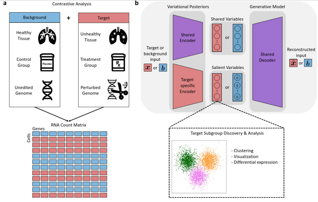
Contrastive VI是一种基于scvi-tools的自编码器生成模型，该模型最早于2023年发布于《Nature Methdos》。旨在从一组“目标”细胞（例如来自患有特定疾病的样本）中分离出特有的变异因素，与一组“背景”细胞（例如来自健康样本的细胞）所共有的因素区分开来。训练时会将背景矩阵与目的矩阵合并为统一矩阵，将每个细胞编码为低维潜在空间中一个分布的参数。可以根据细胞的潜在表示来估计观察到的RNA测量值所基于的分布的参数，分布参数可用于缺失值填补或差异基因表达分析，作者已对不同的药物处理，TP53细胞系等扰动进行了验证，Contrastive VI能够做到有效识别，并提取去噪后的RNA矩阵。这些分布明确考虑了观察数据中的技术因素，如测序深度、批次效应和缺失值。所有分布都由神经网络参数化。训练Contrastive VI将目标细胞特有的潜在变异因素与背景细胞共有的潜在变异因素分离到不同的潜在空间中，并在目标细胞特有的潜在空间上运行聚类算法以发现目标细胞的亚群，使用类似于scVI的程序对发现的目标细胞子群进行差异表达测试。contrastiveVI采用一种概率性潜在变量模型，将观察到的RNA数量中的不确定性表示为生物因素和技术因素的组合。因此，其参数可以通过高效的随机优化技术进行学习，能够轻松适用于包含数万或数十万细胞的大型scRNA-seq数据集。

简单来说，可以完成一种“更高级”的差异分析，能够识别更细微的单细胞差异。需要注意的是，github的版本已经不再更新维护了，最新的教程可以参考scvi-tools上发布的版本[1]。

更多课程：

Python版scRNA-seq分析全流程

Python 空间转录组全程班

如果需要单细胞数据分析指导、生信热点全文复现、自测数据个性化分析辅导、常态化实验学习，欢迎联系客服微信[Biomamba_zhushou]。

二、实操流程

（1）安装配置Contrastive VI环境

实测官网的直接用pip和conda安装方式会报错，推荐大家参考我们的方式通过结合conda和pip配置并管理对应环境，conda安装使用技巧可见：生信软件管家——conda的安装、使用、卸载。

# 创建环境：
mamba  env create -f contrastiveVI-main/environment.yml
# 激活环境
conda activate contrastive-vi-env
# 安装contrastive-vi
pip install contrastive-vi -i https://pypi.tuna.tsinghua.edu.cn/simple

# 进入Python交互环境，测试导入
import contrastive_vi
from contrastive_vi.model import ContrastiveVI
import scvi
import pytorch_lightning
# 如果你导入失败，请记得检查自己的版本是否与我的一致
print(f'scvi版本：{scvi.__version__}')
print(f'pytorch_lightning版本：{pytorch_lightning.__version__}')
print(f'contrastive_vi版本：{contrastive_vi.__version__}')

scvi版本：0.16.1 

pytorch_lightning版本：1.5.10.post0 

contrastive_vi版本：0.2.0

如果你使用Jupyter参与本教程的学习，可参考以下教程安装配置：
码Python神器：jupyter notebook
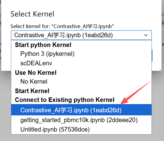
jupyter如何切换内核
JupyterHub：多人使用jupyter的最佳选择
我这里用的是jupyterHub，可以如是提交镜像：

# 安装ipykernel依赖
mamba install ipykernel -y
# 把环境注册为Jupyter Kernel，name为conda环境的名称、display-name为jupyter中实际展示的名称
python -m ipykernel install --user --name contrastive-vi-env --display-name "contrastive_VI教程"

内核布置成功后，能够在jupyter的kernel中找到你提交的环境名称：

（2）急性白血病演示数据

2.1 数据概况

急性髓系白血病（AML）是一种影响骨髓和血液的癌症。急性髓系白血病（AML）的一种治疗选择是造血干细胞移植。在这种疗法中，患者骨髓中的细胞通过化疗或放疗被摧毁，然后将健康的干细胞移植到骨髓中，以重新建立血细胞生成过程。 该数据由从AML患者移植前后采集的骨髓单核细胞的测量值组成。正如先前的研究指出的那样，这些数据中的大部分变异并非由移植前与移植后的状态差异造成，因此很难区分这两组细胞。在此，我们展示了如何利用对比变分自编码器（contrastiveVI）来实现这一区分，方法是从健康患者和癌症患者的细胞中共享的变异中分离出特定于移植状态的变异。

# 数据下载
!gdown --id "1-QRE2up3YecF2yrMj1bd_SUQXF_w0RDZ" # Downloads the preprocessed data
# 你大概率会被墙，不过我们在本地给大家准备好了测试文件

# 加载所需要的包
from contrastive_vi.model import ContrastiveVI
from pytorch_lightning.utilities.seed import seed_everything
import scanpy as sc
seed_everything(42) # 设置全局随机数，保证结果可重复性

Global seed set to 42

42

# 数据读取
adata = sc.read_h5ad("data/zheng_2017.h5ad")
# 预处理：
ContrastiveVI.setup_anndata(adata, layer="count")# ContrastiveVI能够自动识别GPU参与计算

# 这个数据的分类变量为'condition'：
adata.obs['condition'].unique()# 包含'healthy', 'post_transplant', 'pre_transplant'三种状态

['pre_transplant', 'post_transplant', 'healthy'] 

Categories (3, object): ['healthy', 'post_transplant', 'pre_transplant']

我们旨在弄清楚急性髓系白血病患者细胞与健康对照患者细胞之间的差异，因此我们将数据分为两个部分：一个背景数据集(background_data)，其中包含来自健康对照患者细胞的测量数据；另一个目标数据集(target_adata)，其中包含来自急性髓系白血病患者细胞的测量数据(即post_transplant、pre_transplant)。

# AMI患者：
target_adata = adata[adata.obs["condition"] != "healthy"].copy()
# 健康对照患者：
background_adata = adata[adata.obs["condition"] == "healthy"].copy()

# 看一下数据概况
import scanpy as sc
import matplotlib.pyplot as plt
# PCA降维：
sc.pp.pca(target_adata)
# PCA可视化：
fig, ax1 = plt.subplots(1, 1, figsize=(5,5), gridspec_kw={'wspace':0.7})# 设置绘图参数
ax1 = sc.pl.pca(target_adata, color='condition', ax=ax1, title="Transplant Status")# 可视化
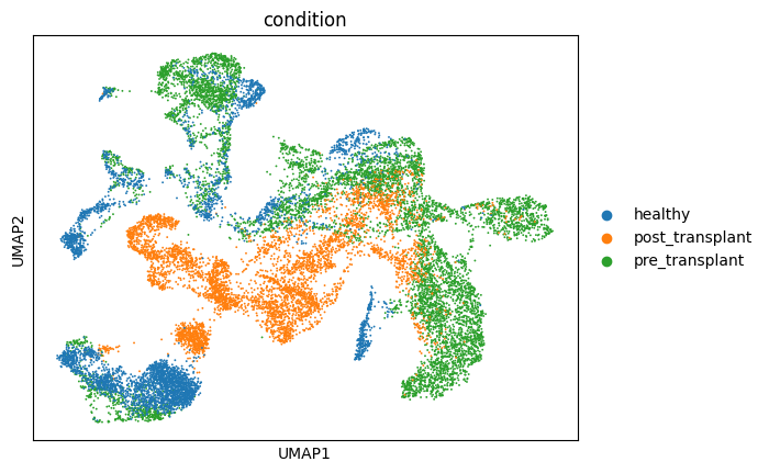
# 寻找临近点：
sc.pp.neighbors(adata, n_neighbors=10, n_pcs=40)
# umap降维计算：
sc.tl.umap(adata)
# umap可视化：
sc.pl.umap(adata, color='condition')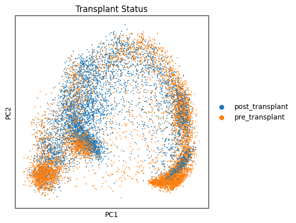

/data2/analysis/biomamba_tutor/miniconda3/envs/contrastive-vi-env/lib/python3.9/site-packages/scanpy/tools/_utils.py:41: UserWarning: You’re trying to run this on 2000 dimensions of `.X`, if you really want this, set `use_rep='X'`.

          Falling back to preprocessing with `sc.pp.pca` and default params.

   warnings.warn(

2.2 训练数据

为了实现这区别，我们先利用之前完整标注的数据，通过contrastiveVI表构建模型。

model = ContrastiveVI(
    adata,
    n_salient_latent=10,
    n_background_latent=10,
    use_observed_lib_size=False
)                         

INFO   contrastive_vi: The model has been initialized      

告诉模型我们需要比较background与target, 并进行训练

# 导入numpy
import numpy as np
# 背景细胞的索引：
background_indices = np.where(adata.obs["condition"] == "healthy")[0]
# AMI患者细胞的索引
target_indices = np.where(adata.obs["condition"] != "healthy")[0]
background_indices

array([12399, 12400, 12401, ..., 16853, 16854, 16855])

下面我们使用GPU与CPU两种方式进行训练，可以看出GPU仅花费6min，而CPU花费了5h，计算效率高下立判。需要GPU的小伙伴可参考：RTX5090、4080S、5070显卡上机。

%%time
# GPU训练
model.train(
    check_val_every_n_epoch=1,# 每 n 个训练轮次（epoch）执行一次验证集评估，监控模型泛化能力，设为1表示每个epoch都验证，便于及时观察验证集指标变化
    train_size=0.8,# 训练集比例
    background_indices=background_indices,# 背景样本的索引
    target_indices=target_indices,# AMI患者细胞的索引
    use_gpu=True, # 是否使用GPU
    early_stopping=True,# 是否启用早停策略（防止模型过拟合）。启用后，若验证集指标连续多轮无提升，会提前终止训练，避免无效训练。
    max_epochs=500,# 模型训练的最大轮数（epoch），若未触发早停，训练会在达到该轮数后停止；若触发早停则提前终止
)

GPU available: True, used: True 

TPU available: False, using: 0 TPU cores 

IPU available: False, using: 0 IPUs 

LOCAL_RANK: 0 - CUDA_VISIBLE_DEVICES: [0]

Epoch 228/500:  46%|████▌     | 228/500 [07:51<09:22,  2.07s/it, loss=803, v_num=1]  

Monitored metric elbo_validation did not improve in the last 45 records. Best score: 907.662. 

Signaling Trainer to stop. 

CPU times: user 7min 49s, sys: 1.23 s, total: 7min 50s 

Wall time: 7min 51s

%%time
# CPU训练
model.train(
    check_val_every_n_epoch=1,
    train_size=0.8,
    background_indices=background_indices,
    target_indices=target_indices,
    use_gpu=False, 
    early_stopping=True,
    max_epochs=500,
)

GPU available: True, used: False 

TPU available: False, using: 0 TPU cores 

IPU available: False, using: 0 IPUs 

/data2/analysis/biomamba_tutor/miniconda3/envs/contrastive-vi-env/lib/python3.9/site-packages/pytorch_lightning/trainer/trainer.py:1584: UserWarning: GPU available but not used. Set the gpus flag in your trainer `Trainer(gpus=1)` or script `--gpus=1`.

   rank_zero_warn(

Epoch 126/500:  25%|██▌       | 126/500 [5:09:21<15:18:15, 147.31s/it, loss=777, v_num=1] Monitored metric elbo_validation did not improve in the last 45 records. Best score: 934.355. Signaling Trainer to stop. 

CPU times: user 15d 1h 17min 3s, sys: 24min 19s, total: 15d 1h 41min 23s 

Wall time: 5h 9min 21s

利用我们训练好的模型，我们将把接触了idasanutlin处理的细胞嵌入到共享的潜在空间以及针对特定目标（显著特征）的潜在空间中。

from anndata import AnnData
salient_adata = AnnData(
    X=model.get_latent_representation(target_adata, representation_kind='salient'),
    obs=target_adata.obs
)

INFO     AnnData object appears to be a copy. Attempting to transfer setup.                  

# 这时你就可以看出post_transplant和pre_transplant之间的降维差别：
sc.pp.pca(salient_adata)
fig, ax1 = plt.subplots(1, 1, figsize=(5,5), gridspec_kw={'wspace':0.7}) # 设置绘图参数
sc.pl.pca(salient_adata, color='condition', ax=ax1, title="Transplant Status") # pca降维图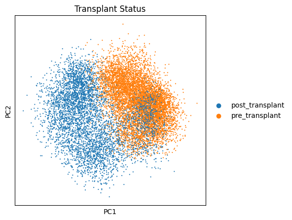

# 寻找临近点：
sc.pp.neighbors(salient_adata, n_neighbors=10, n_pcs=40)
# umap降维计算：
sc.tl.umap(salient_adata)
# umap可视化：
sc.pl.umap(salient_adata,color='condition')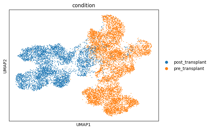

我们还可以通过调整后的兰德指数（ARI）来量化不同感染类型下细胞分离的效果。该指数的取值范围在 0 到 1 之间，分数越高表明分离效果越好。

from sklearn.metrics import adjusted_rand_score
from sklearn.cluster import KMeans
clustering_labels = KMeans(n_clusters=2).fit(salient_adata.X).labels_ # 获得label标签
ari = adjusted_rand_score(target_adata.obs["condition"], clustering_labels) # 计算rand指数
print(ari)

0.7573400579411594

（3）识别肠道上皮细胞的感染类型

在许多生物学内容中，最佳的思路是找到疾病群体中存在、而健康群体中不存在的变异。为了展示contrastiveVI能够如何识别这种变异，作者演示了一个Salmonella或H. polygyrus感染及健康未感染的肠道上皮细胞。

3.1 数据概况

# 数据下载
!gdown --id "1-QRE2up3YecF2yrMj1bd_SUQXF_w0RDZ" # Downloads the preprocessed data
# 你大概率会被墙，不过我们在本地给大家准备好了测试文件

# 导包
from contrastive_vi.model import ContrastiveVI
from pytorch_lightning.utilities.seed import seed_everything
import scanpy as sc
seed_everything(123) # 设置随机数保证结果可重复
# 读取数据：
adata = sc.read_h5ad("./data/haber_2017.h5ad")
# 预处理：
ContrastiveVI.setup_anndata(adata, layer="count")

Global seed set to 123

# 数据共包含7721个细胞
adata.obs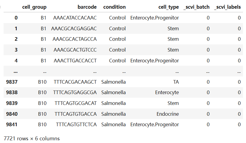

adata.obs['condition'].unique()# 该数据共有三个分组

['Control', 'Hpoly.Day10', 'Salmonella'] Categories (3, object): ['Control', 'Hpoly.Day10', 'Salmonella']

与上一个教程类似，这里分隔出感染、未感染的两个对象

# 不等于control的即为感染对象：
target_adata = adata[adata.obs["condition"] != "Control"].copy()
# 等于Control的是作为背景的健康对象：
background_adata = adata[adata.obs["condition"] == "Control"].copy()

### 展示感染类型和细胞类型的UMAP图 ###
# 导包：
import matplotlib.pyplot as plt
# 计算临近点：
sc.pp.neighbors(target_adata)
# 计算umap降维：
sc.tl.umap(target_adata)
#  可视化umap
fig, (ax1, ax2) = plt.subplots(1, 2, figsize=(10,5), gridspec_kw={'wspace':0.7})
ax1 = sc.pl.umap(target_adata, color='condition', ax=ax1, title="Infection", show=False)
ax2 = sc.pl.umap(target_adata, color='cell_type', title="Cell Type", ax=ax2)

/data2/analysis/biomamba_tutor/miniconda3/envs/contrastive-vi-env/lib/python3.9/site-packages/scanpy/tools/_utils.py:41: UserWarning: You’re trying to run this on 2000 dimensions of `.X`, if you really want this, set `use_rep='X'`.          Falling back to preprocessing with `sc.pp.pca` and default params.   warnings.warn(

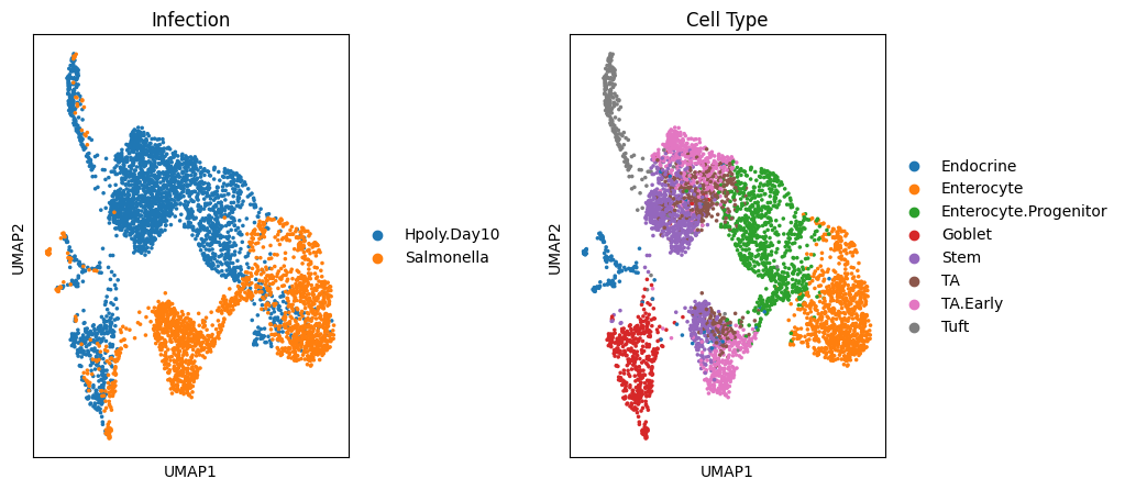
哪个生信人不想不同变量之间分离的比较开呢，但实际上总是事与愿违，可以看出，无论是感染类型之间、还是细胞类型之间，细胞都存在互相粘连的情况。

3.2 训练数据

# 构建模型：
model = ContrastiveVI(
    adata,
    n_salient_latent=10,
    n_background_latent=10,
    use_observed_lib_size=False
)

INFO     contrastive_vi: The model has been initialized                                                  

### 训练backgroun vs target的模型 ###
# 导包
import numpy as np
# 获得background和target的索引：
background_indices = np.where(adata.obs["condition"] == "Control")[0]
target_indices = np.where(adata.obs["condition"] != "Control")[0]
# 训练模型，具体参数介绍见上一章
model.train(
    check_val_every_n_epoch=1,
    train_size=0.8,
    background_indices=background_indices,
    target_indices=target_indices,
    use_gpu=True,
    early_stopping=True,
    max_epochs=500,
)

GPU available: True, used: True 

TPU available: False, using: 0 TPU cores 

IPU available: False, using: 0 IPUs 

LOCAL_RANK: 0 - CUDA_VISIBLE_DEVICES: [0]

Epoch 2/500:   0%|          | 1/500 [00:00<06:11,  1.34it/s, loss=6.64e+03, v_num=1]

/data2/analysis/biomamba_tutor/miniconda3/envs/contrastive-vi-env/lib/python3.9/site-packages/pytorch_lightning/utilities/data.py:59: UserWarning: Trying to infer the `batch_size` from an ambiguous collection. The batch size we found is 8. To avoid any miscalculations, use `self.log(..., batch_size=batch_size)`.

   warning_cache.warn(

Epoch 399/500:  80%|███████▉  | 399/500 [04:57<01:15,  1.34it/s, loss=1.02e+03, v_num=1] 

Monitored metric elbo_validation did not improve in the last 45 records. Best score: 1066.963. Signaling Trainer to stop.

现在，利用我们训练好的模型，我们将把受感染的细胞嵌入到共享的潜在空间以及针对特定目标的（显著的）潜在空间中。

target_adata.obsm['salient_rep'] = model.get_latent_representation(target_adata, representation_kind='salient')
target_adata.obsm['background_rep'] = model.get_latent_representation(target_adata, representation_kind='background')

INFO     AnnData object appears to be a copy. Attempting to transfer setup.                     

### 处理后的降维 ###
sc.pp.neighbors(target_adata, use_rep="salient_rep")
sc.tl.umap(target_adata, min_dist=0.1)
fig, (ax1, ax2) = plt.subplots(1, 2, figsize=(10,5), gridspec_kw={'wspace':0.7})
sc.pl.umap(target_adata, color='condition', ax=ax1, title="Infection", show=False)
sc.pl.umap(target_adata, color='cell_type', ax=ax2, title="Cell Type")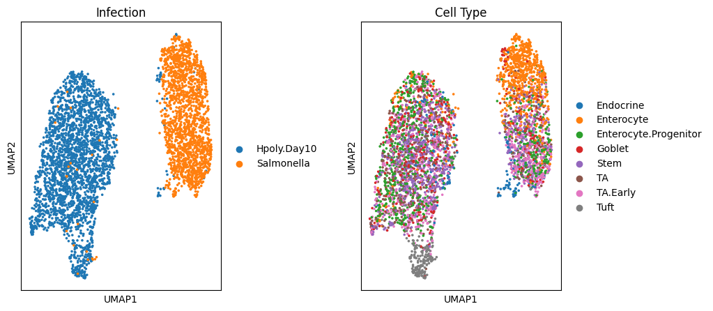

### 处理前的降维，高下立判 ###
sc.pp.neighbors(target_adata, use_rep="background_rep")
sc.tl.umap(target_adata, min_dist=0.1)
fig, (ax1, ax2) = plt.subplots(1, 2, figsize=(10,5), gridspec_kw={'wspace':0.7})
sc.pl.umap(target_adata, color='condition', ax=ax1, title="Infection", show=False)
sc.pl.umap(target_adata, color='cell_type', ax=ax2, title="Cell Type")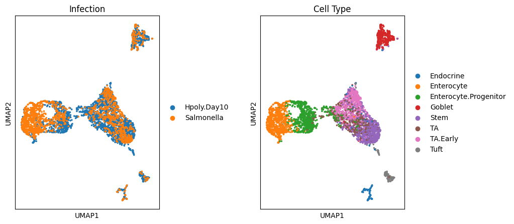

可视化一下，可以看出感染类型之间的分隔已经非常明显了，这里我们也给大家留一个小作业，如何实现展示各细胞类型的差异？

###  adjusted rand index (ARI)评估分离效果. 结果取值0到1,越高则代表分离度越好 ###
from sklearn.metrics import adjusted_rand_score
from sklearn.cluster import KMeans
clustering_labels = KMeans(n_clusters=2).fit(target_adata.obsm['salient_rep']).labels_
ari = adjusted_rand_score(target_adata.obs["condition"], clustering_labels)
print(ari)

0.8955993857049277

（4）解析阿尔兹海默症异质性响应

4.1 数据概况

阿尔茨海默病（AD）是老年人群中最常见的痴呆症类型。由于老年人的临床病理状态存在极大的差异，且关于AD的潜在遗传和分子驱动因素的知识有限，目前尚未有能够预防、治愈或延缓其病情进展的治疗方法。本教程利用contrastive VI来更好地理解阿尔茨海默病的转录反应多样性，具体方法是将其应用于格鲁布曼等人的一项单细胞RNA测序数据集。该数据集测量了来自六名确诊患有阿尔茨海默病的死后个体的杏仁核组织中的表达水平。背景数据集使用了来自同一研究中六名年龄和性别匹配的健康对照个体的测量值。

# 下载数据：
!gdown --id "1R1aN-LWUQ6c_N44n5-xjy2nEPzl7H0Dc"
# 你大概率会被墙，不过我们准备好了对应的数据

from contrastive_vi.model import ContrastiveVI
import scanpy as sc
# 读取数据：
adata = sc.read_h5ad("./data/grubman_2019.h5ad")
# 预处理：
ContrastiveVI.setup_anndata(adata, layer="count")

# 这个数据共分为'Alzheimer'和'control'组：
adata.obs['batchCond'].unique()

['AD', 'ct'] 

Categories (2, object): ['AD', 'ct']

4.2 训练数据

# 构建模型：
model = ContrastiveVI(
    adata,
    n_salient_latent=10,
    n_background_latent=10,
    use_observed_lib_size=False
)
# 导包：
import numpy as np
# 背景数据的索引：
background_indices = np.where(adata.obs["batchCond"] == "ct")[0]
# 目标数据的索引
target_indices = np.where(adata.obs["batchCond"] != "ct")[0]
# 训练数据：
model.train(
    check_val_every_n_epoch=1,
    train_size=0.8,
    background_indices=background_indices,
    target_indices=target_indices,
    early_stopping=True,
    max_epochs=500,
)

INFO     contrastive_vi: The model has been initialized                                                         

GPU available: True, used: True T

PU available: False, using: 0 TPU cores 

IPU available: False, using: 0 IPUs 

LOCAL_RANK: 0 - CUDA_VISIBLE_DEVICES: [0]

Epoch 2/500:   0%|          | 1/500 [00:01<10:06,  1.22s/it, loss=2.29e+03, v_num=1]

/data2/analysis/biomamba_tutor/miniconda3/envs/contrastive-vi-env/lib/python3.9/site-packages/pytorch_lightning/utilities/data.py:59: UserWarning: Trying to infer the `batch_size` from an ambiguous collection. The batch size we found is 72. To avoid any miscalculations, use `self.log(..., batch_size=batch_size)`.

   warning_cache.warn(

Epoch 337/500:  67%|██████▋   | 337/500 [06:28<03:07,  1.15s/it, loss=903, v_num=1]  

Monitored metric elbo_validation did not improve in the last 45 records. Best score: 931.414. Signaling Trainer to stop.

# 获得目标数据：
target_adata = adata[adata.obs["batchCond"] != "ct"].copy()
# 获得背景数据：
background_adata = adata[adata.obs["batchCond"] == "ct"].copy()
# 提取target的关键潜在特征
target_adata.obsm['salient_rep'] = model.get_latent_representation(target_adata, representation_kind='salient')
# 提取背景的关键潜在特征：
target_adata.obsm['background_rep'] = model.get_latent_representation(target_adata, representation_kind='background')

INFO     AnnData object appears to be a copy. Attempting to transfer setup.                     

# 获得目标数据：
target_adata = adata[adata.obs["batchCond"] != "ct"].copy()
# 获得背景数据：
background_adata = adata[adata.obs["batchCond"] == "ct"].copy()
# 提取target的关键潜在特征
target_adata.obsm['salient_rep'] = model.get_latent_representation(target_adata, representation_kind='salient')
# 提取背景的关键潜在特征：
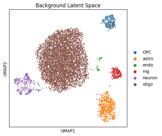
target_adata.obsm['background_rep'] = model.get_latent_representation(target_adata, representation_kind='background')

<Axes: title={'center': 'Background Latent Space'}, xlabel='UMAP1', ylabel='UMAP2'>

# # 安装分群依赖包
!pip install igraph 
!pip install leidenalg

### 依据目标特征的潜在降维图 ###
# 计算临近值：
sc.pp.neighbors(target_adata, use_rep="salient_rep")
# 计算umap：
sc.tl.umap(target_adata)
# 分群
sc.tl.leiden(target_adata, resolution=0.25)
# umap可视化：
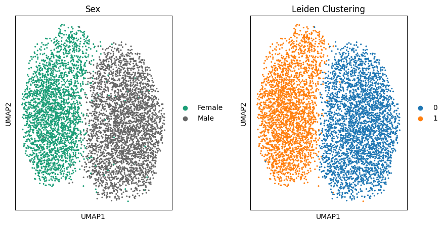
fig, (ax1, ax2) = plt.subplots(1, 2, figsize=(10,5), gridspec_kw={'wspace':0.7})
# 此时各细胞类型的umap较为混合：
sc.pl.umap(target_adata, color='cellType', ax=ax1, title="Salient Latent Space", show=False)
# 基于salient_rep的leiden分群展示出了新的分群
sc.pl.umap(target_adata, color='leiden', ax=ax2, title="Leiden Clustering", show=False)

/tmp/ipykernel_961019/4262007672.py:8: FutureWarning: In the future, the default backend for leiden will be igraph instead of leidenalg. 

  To achieve the future defaults please pass: flavor="igraph" and n_iterations=2.  directed must also be False to work with igraph's implementation.

   sc.tl.leiden(target_adata, resolution=0.25)

<Axes: title={'center': 'Leiden Clustering'}, xlabel='UMAP1', ylabel='UMAP2'>

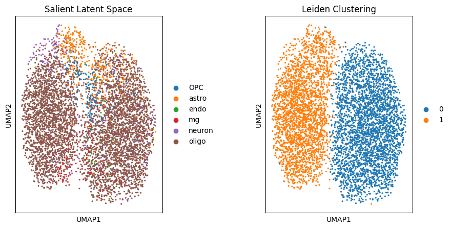
根据作者提供的变量，我们发现这一分群与性别呈现出很强的关联

fig, (ax1, ax2) = plt.subplots(1, 2, figsize=(10,5), gridspec_kw={'wspace':0.5})
sc.pl.umap(target_adata, color='sex', ax=ax1, title="Sex", show=False, palette="Dark2")
sc.pl.umap(target_adata, color='leiden', ax=ax2, title="Leiden Clustering", show=False)

<Axes: title={'center': 'Leiden Clustering'}, xlabel='UMAP1', ylabel='UMAP2'>

4.3 基于contrastive VI的差异分析

# 导包
from tqdm import tqdm
# 创建空字典：
de_results = {}
top_genes_per_cell_type = {}  
# 循环计算每个细胞的组间差异分析
for cell_type in tqdm(adata.obs['cellType'].unique()):
    if cell_type == 'endo': # endo细胞数量过低，因此跳过
        continue
    # 取出对应细胞的对象切片，防止造成原对象的结构更改：
    adata_tmp = target_adata[target_adata.obs['cellType'] == cell_type].copy()
    # 计算每种细胞类型在sex变量中Male vs Female的差异基因：
    results_tmp = model.differential_expression(
        adata=adata_tmp,
        groupby="sex",
        group1="Male",
        group2="Female",
        idx1=None,# # 手动指定group1的细胞索引（None则自动按groupby筛选）
        idx2=None,# 手动指定group2的细胞索引（None则自动按groupby筛选）
        mode="change",# 计算表达变化量
        batch_size=128,# 批次处理大小，内存或现存不够的时候可以调整的小一些
        all_stats=True,# 是否返回所有统计指标
        batch_correction=False,# 是否做批次矫正
        batchid1=None,# 批次1，None则为不做批次矫正
        batchid2=None,# 批次2，None则为不做批次矫正
        fdr_target=0.05,# FDR阈值
        silent=False, #是否静默运行（False则输出分析过程）
    )
    results_tmp = results_tmp[results_tmp['proba_de'] > 0.95] # # proba_de：contrastiveVI输出的“基因为差异表达的概率”（0~1），>0.95表示极高置信度
    top_genes_per_cell_type[cell_type] = results_tmp.index[:10]# 筛选每个细胞类型的top 10基因
    de_results[cell_type] = set(results_tmp.index)# 存储每个细胞类型的top基因
# 对de_results中所有细胞类型的差异基因集合取交集
de_genes_all_cell_types = set.intersection(*de_results.values())
# 差异计算还是比较慢的，需要有一定耐心

 0%|          | 0/6 [00:00<?, ?it/s]

INFO     AnnData object appears to be a copy. Attempting to transfer setup.   

DE...: 100%|██████████| 1/1 [00:33<00:00, 33.83s/it]

/data2/analysis/biomamba_tutor/miniconda3/envs/contrastive-vi-env/lib/python3.9/site-packages/scvi/model/base/_utils.py:284: FutureWarning: Series.__getitem__ treating keys as positions is deprecated. In a future version, integer keys will always be treated as labels (consistent with DataFrame behavior). To access a value by position, use `ser.iloc[pos]`

   sorted_pgs = posterior_probas[sorted_genes]

  17%|█▋        | 1/6 [00:33<02:49, 33.98s/it]

INFO     AnnData object appears to be a copy. Attempting to transfer setup.         

DE...: 100%|██████████| 1/1 [00:33<00:00, 33.77s/it]

/data2/analysis/biomamba_tutor/miniconda3/envs/contrastive-vi-env/lib/python3.9/site-packages/scvi/model/base/_utils.py:284: FutureWarning: Series.__getitem__ treating keys as positions is deprecated. In a future version, integer keys will always be treated as labels (consistent with DataFrame behavior). To access a value by position, use `ser.iloc[pos]`

   sorted_pgs = posterior_probas[sorted_genes]

  33%|███▎      | 2/6 [01:07<02:15, 33.87s/it]

INFO     AnnData object appears to be a copy. Attempting to transfer setup.     

DE...: 100%|██████████| 1/1 [00:33<00:00, 33.74s/it]

/data2/analysis/biomamba_tutor/miniconda3/envs/contrastive-vi-env/lib/python3.9/site-packages/scvi/model/base/_utils.py:284: FutureWarning: Series.__getitem__ treating keys as positions is deprecated. In a future version, integer keys will always be treated as labels (consistent with DataFrame behavior). To access a value by position, use `ser.iloc[pos]`

   sorted_pgs = posterior_probas[sorted_genes]  

50%|█████     | 3/6 [01:41<01:41, 33.82s/it]

INFO     AnnData object appears to be a copy. Attempting to transfer setup.   

DE...: 100%|██████████| 1/1 [00:33<00:00, 33.77s/it]

/data2/analysis/biomamba_tutor/miniconda3/envs/contrastive-vi-env/lib/python3.9/site-packages/scvi/model/base/_utils.py:284: FutureWarning: Series.__getitem__ treating keys as positions is deprecated. In a future version, integer keys will always be treated as labels (consistent with DataFrame behavior). To access a value by position, use `ser.iloc[pos]`

   sorted_pgs = posterior_probas[sorted_genes]

  67%|██████▋   | 4/6 [02:15<01:07, 33.81s/it]

INFO     AnnData object appears to be a copy. Attempting to transfer setup.         

DE...: 100%|██████████| 1/1 [00:33<00:00, 33.71s/it]

/data2/analysis/biomamba_tutor/miniconda3/envs/contrastive-vi-env/lib/python3.9/site-packages/scvi/model/base/_utils.py:284: FutureWarning: Series.__getitem__ treating keys as positions is deprecated. In a future version, integer keys will always be treated as labels (consistent with DataFrame behavior). To access a value by position, use `ser.iloc[pos]`

   sorted_pgs = posterior_probas[sorted_genes] 

100%|██████████| 6/6 [02:49<00:00, 28.18s/it]

adata.obs['cellType'].unique()

['oligo', 'astro', 'OPC', 'neuron', 'endo', 'mg'] Categories (6, object): ['OPC', 'astro', 'endo', 'mg', 'neuron', 'oligo']

adata.obs['cellType'].unique()
    if cell_type == 'endo': # endo细胞数量过低，因此跳过
        continue
    # 取出对应细胞的对象切片，防止造成原对象的结构更改：

{'ELOVL2', 'F13A1', 'GMFB', 'GPR63', 'MT-CO2', 'MYO5B'}

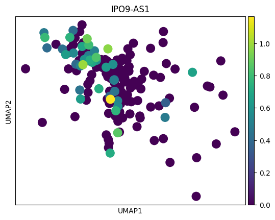
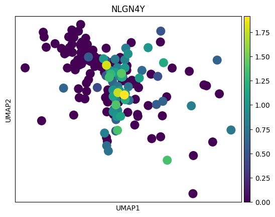
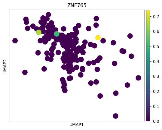
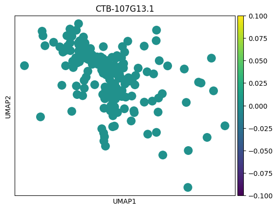
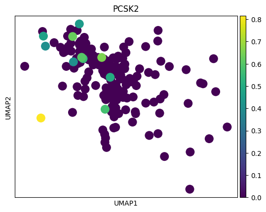
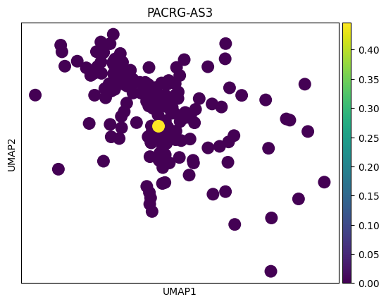
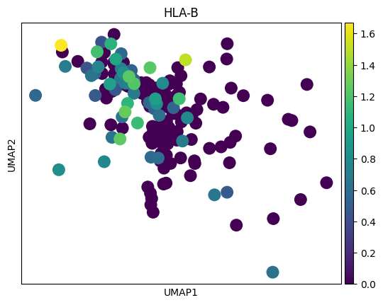
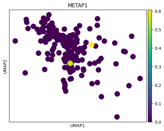
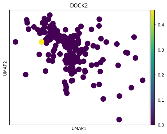
差异基因可视化

genes

Index(['GPR63', 'IPO9-AS1', 'NLGN4Y', 'ZNF765', 'CTB-107G13.1', 'PCSK2',

          'PACRG-AS3', 'HLA-B', 'METAP1', 'DOCK2'],

          dtype='object')

target_adata.obs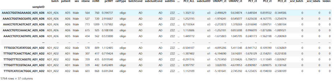

print(target_adata.obsm.keys())

KeysView(AxisArrays with keys: salient_rep, background_rep, X_umap)

adata_tmp = target_adata[target_adata.obs['cellType'] == 'OPC'].copy()
adata_tmp

AnnData object with n_obs × n_vars = 179 × 2000

     obs: 'batch', 'patient', 'sex', 'nGene', 'nUMI', 'pctMT', 'cellType', 'batchCond', 'subclustCond', 'subIDm', 'subIDa', 'subIDn', 'subIDo', 'subIDO', 'subIDe', 'subIDu', 'subIDh', 'mg', 'astro', 'neuron', 'oligo', 'OPC', 'endo', 'UMAP1_ALL', 'UMAP2_ALL', 'PC1_ALL', 'PC2_ALL', 'PC3_ALL', 'subclustID', 'UMAP1_ct', 'UMAP2_ct', 'PC1_ct', 'PC2_ct', 'PC3_ct', '_scvi_batch', '_scvi_labels', 'leiden'

     var: 'highly_variable', 'highly_variable_rank', 'means', 'variances', 'variances_norm'

     uns: 'hvg', '_scvi_uuid', '_scvi_manager_uuid', 'neighbors', 'umap', 'cellType_colors', 'leiden', 'leiden_colors', 'sex_colors'

     obsm: 'salient_rep', 'background_rep', 'X_umap'

     layers: 'count'

     obsp: 'distances', 'connectivities'

# 导包
from anndata import AnnData
# 获取标准化后的矩阵
adata_normalized = AnnData(
    X=model.get_normalized_expression(target_adata)['salient'],
    obs=target_adata.obs,
    var=target_adata.var
)
# 做切片查看OPC的差异基因
adata_tmp = target_adata[target_adata.obs['cellType'] == 'OPC'].copy()
axes_flat = [item for sublist in axs for item in sublist]
genes = top_genes_per_cell_type['OPC']
fontsize = 24
sc.pl.umap(adata_tmp,color = 'sex')
for gene in genes:
    sc.pl.umap(adata_tmp,color = gene)
# 感觉这里作者有点翻车，对应差异基因在两种sex间并未展现出很明显的差异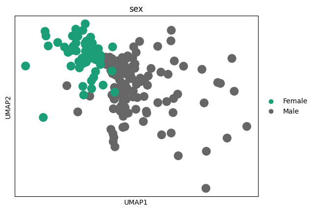

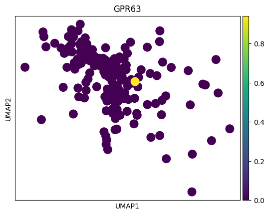
# 倒是作者给了几个基因，在sex间的差异倒是挺大
fig, axs = plt.subplots(2, 2, figsize=(10, 10))
cmap = 'magma'
axes_flat = [item for sublist in axs for item in sublist]
genes = ['HSPA1A', 'DNAJB1', 'LINGO1', 'BOK']
fontsize = 24
for ax, gene in zip(axes_flat, genes):
    s = ax.scatter(
        target_adata.obsm['X_umap'][:, 0],
        target_adata.obsm['X_umap'][:, 1],
        c=adata_normalized[:, gene].X.reshape(-1),
        cmap=cmap,
        s=3
    )
    ax.set_title(gene, fontsize=fontsize)
    ax.set_xticks([])
    ax.set_yticks([])
cbar = fig.colorbar(s, ax=axes_flat)
cbar.set_ticks([])
cbar.ax.set_title("High", fontsize=fontsize)
cbar.set_label("Low    ", rotation=0, y=-0.01, fontsize=fontsize)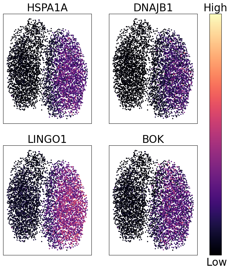

三、参考

[1]Ethan Weinberger, Chris Lin, Su-In Lee (2023), Isolating salient variations of interest in single-cell data with contrastiveVI, Nature Methods.

[2]https://docs.scvi-tools.org/en/stable/installation.html

[3]https://www.nature.com/articles/s41467-020-17440-w

四、资料领取

更多编程教程可见：

十小时学会Linux

5.5小时掌握R语言

生信python速查手册

一切不给测试文件和分析环境版本的教程都是耍流氓，本推送的代码和测试文件可以在以下链接中下载：

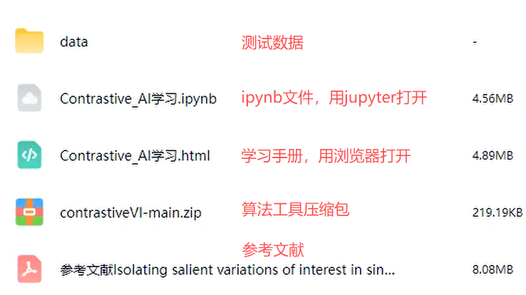
链接: https://pan.baidu.com/s/1-1kNq7mMJC60_3UTARnx3A

提取码: uw9n