深度学习实战-基于Xception的阿尔茨海默病图像识别模型
🤵♂️ 个人主页:@艾派森的个人主页
✍🏻作者简介:Python学习者
🐋 希望大家多多支持,我们一起进步!😄
如果文章对你有帮助的话,
欢迎评论 💬点赞👍🏻 收藏 📂加关注+
目录
1.项目背景
阿尔茨海默病作为最常见的神经退行性疾病之一,早期诊断对延缓病情进展和提高患者生活质量具有重要意义。临床上,脑部磁共振成像(MRI)是评估脑结构变化、辅助诊断的重要工具,能够显示海马体萎缩、脑室扩大等与疾病相关的典型征象。然而,传统影像诊断依赖放射科医生的经验判断,不同医生之间可能存在解读差异,且早期病变的细微特征不易被肉眼准确识别。随着医疗影像数字化程度的提高,积累了大量患者MRI数据,如何利用这些影像资料实现客观、标准化的疾病评估成为研究热点。深度学习技术,特别是卷积神经网络,在医学图像分析领域展现出显著优势。这些模型能够从像素级数据中自动学习疾病的影像特征模式,不受主观经验影响,有望为阿尔茨海默病的早期识别提供新的技术支持。基于MRI图像的自动分类系统不仅可以辅助临床医生提高诊断效率和一致性,还能为疾病进展监测和疗效评估提供量化参考。
本项目核心技术采用基于Xception架构的迁移学习策略。Xception是一种高效的深度可分离卷积神经网络,通过将标准卷积分解为深度卷积和逐点卷积两个步骤,在保持较强特征提取能力的同时显著减少了模型参数量。这种设计使其特别适合处理医学图像这类需要精细特征分析的任务。我们以在ImageNet大型图像数据集上预训练的Xception模型为基础,保留其底层通用特征提取能力,替换顶部分类层并针对阿尔茨海默病四分类任务进行微调训练。结合全局平均池化、Dropout正则化以及自适应学习率调整等策略,构建了一个能够从脑部MRI图像中自动识别不同痴呆程度的分类模型,为临床辅助诊断提供了一种可行的技术路径。
2.数据集介绍
本实验数据集来源于Kaggle,数据包括 MRI 图像。数据分为四类图像,既有训练图像,也有测试集:
- Mild Demented 轻度痴呆
- Moderate Demented 中度痴呆
- Non Demented 非痴呆
- Very Mild Demented 非常轻度的痴呆
数据包含两个文件夹。其中一个是增强版,另一个是原版。
3.技术工具
Python版本:3.9
代码编辑器:jupyter notebook
4.实验过程
4.1导入数据
首先完成实验环境的搭建工作,导入处理阿尔茨海默病MRI图像所需的各类工具库。我们选择了Xception预训练模型作为核心架构,并准备了完整的数据处理和模型训练工具链。
import warnings  # 警告处理模块
warnings.filterwarnings('ignore')  # 忽略警告信息,使输出更清晰

# 导入数据操作和分析库
import pandas as pd  # 数据分析库,用于处理表格数据
import numpy as np  # 数值计算库,用于数组和矩阵运算
import os  # 操作系统接口,用于文件和目录操作
import glob as gb  # 文件路径匹配,用于批量查找图像文件
import cv2  # OpenCV计算机视觉库,用于图像处理

# 导入数据可视化库
import matplotlib.pyplot as plt  # 基础绘图库
import seaborn as sns  # 统计图形库,提供更美观的可视化效果

# 导入机器学习工具
from sklearn.model_selection import train_test_split  # 数据集划分工具
from sklearn.metrics import confusion_matrix  # 混淆矩阵计算

# 导入TensorFlow深度学习框架相关模块
import tensorflow as tf  # TensorFlow主库
from tensorflow.keras.applications import Xception  # Xception预训练模型
from tensorflow.keras.callbacks import EarlyStopping, ReduceLROnPlateau, ModelCheckpoint  # 训练回调函数

# 设置Seaborn绘图主题和调色板
sns.set_theme(style='darkgrid', palette='pastel')  # 使用深色网格风格和柔和调色板
color = sns.color_palette(palette='pastel')  # 获取调色板颜色

# 配置GPU设备(如果可用)
gpus = tf.config.experimental.list_physical_devices('GPU')  # 检测可用GPU设备
接着定义了数据集路径和关键参数,并实现了读取MRI图像数据集的函数。针对阿尔茨海默病诊断任务,我们需要对脑部MRI图像进行标准化处理。
# 定义数据集路径和训练参数
DATASET_DIR = './augmented-alzheimer-mri-dataset/AugmentedAlzheimerDataset'  # 数据集目录路径
IMG_SIZE = 224  # 图像统一调整尺寸(Xception模型的标准输入尺寸)
BATCH_SIZE = 64  # 每个训练批次包含的图像数量
BUFFER_SIZE = 1000  # 数据缓冲区大小(用于数据打乱)
EPOCHS = 10  # 训练的总轮数

def ReadDataset(data_dir):
    """
    读取数据集目录结构,收集所有图像路径和对应标签
    参数:
        data_dir: 数据集根目录路径
    返回:
        img_paths: 所有图像文件的完整路径列表
        labels: 对应的标签列表(数字编码)
        label_map: 标签映射字典(数字到类别名称)
    """
    img_paths = []  # 初始化图像路径列表
    labels = []  # 初始化标签列表
    label_map = {}  # 初始化标签映射字典

    # 遍历数据集目录中的每个类别文件夹
    # enumerate为每个类别分配一个数字索引
    for idx, folder in enumerate(os.listdir(data_dir)):
        label_map[idx] = folder  # 建立数字索引到类别名称的映射

        # 遍历当前类别文件夹中的子目录或文件
        for path in os.listdir(data_dir + '/' + folder):
            # 使用glob模式匹配获取所有图像文件路径
            files = gb.glob(pathname=str(data_dir + '/' + folder + '/' + path))

            # 将每个图像文件路径和对应标签添加到列表中
            for file in files:
                img_paths.append(file)
                labels.append(idx)  # 使用当前类别索引作为标签

    return np.array(img_paths), np.array(labels), label_map


# 调用函数读取数据集
dataset_paths, dataset_labels, label_map = ReadDataset(DATASET_DIR)

# 计算类别数量
N_CLASSES = len(label_map.keys())

# 打印one-hot编码前的标签形状
print(" Shape before one-hot encoding : ", dataset_labels.shape)

# 将整数标签转换为one-hot编码格式
# one-hot编码将类别标签转换为向量形式,如类别2变为[0,0,1,0,...]
dataset_labels = tf.keras.utils.to_categorical(dataset_labels, N_CLASSES)

# 打印one-hot编码后的标签形状
print(" Shape after one-hot encoding : ", dataset_labels.shape)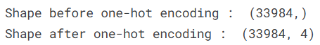
4.2数据预处理
这里我们主要完成MRI数据集的划分、预处理和数据管道构建工作。对于阿尔茨海默病诊断这样的医学图像分析任务,规范化的数据处理流程至关重要,它直接影响模型学习效果和最终诊断准确性。
# 划分训练集和验证集
# train_test_split函数将数据集按照80%训练、20%验证的比例划分
# random_state=42确保每次划分结果一致,便于实验复现
train_data, val_data, train_labels, val_labels = train_test_split(
    dataset_paths,      # 图像路径数组
    dataset_labels,     # one-hot编码的标签数组
    train_size=0.8,     # 训练集占比80%
    random_state=42     # 随机种子
)

def map_fn(img_path, label):
    """
    图像预处理映射函数
    参数:
        img_path: 图像文件路径
        label: 对应标签
    返回:
        处理后的图像张量和标签
    """
    # 读取图像文件
    img = tf.io.read_file(img_path)

    # 解码JPEG格式图像
    img = tf.image.decode_jpeg(img)

    # 调整图像尺寸到224x224像素
    img = tf.image.resize(img, (IMG_SIZE, IMG_SIZE))

    # 将像素值转换为float32类型并归一化到[0,1]范围
    # 除以255.0将0-255的像素值映射到0-1之间
    img = tf.cast(img, tf.float32) / 255.

    return img, label


# 创建训练数据集
# 从张量切片创建数据集,将图像路径和标签配对
train_set = tf.data.Dataset.from_tensor_slices((train_data, train_labels))

# 应用预处理函数到每个样本
train_set = train_set.map(map_fn)

# 打乱数据顺序并设置批次大小
# shuffle: 随机打乱数据,缓冲区大小1000
# batch: 每批64张图像
train_set = train_set.shuffle(BUFFER_SIZE).batch(BATCH_SIZE)

# 创建验证数据集(与训练集类似,但不打乱顺序)
val_set = tf.data.Dataset.from_tensor_slices((val_data, val_labels))
val_set = val_set.map(map_fn)
val_set = val_set.batch(BATCH_SIZE)

# 打印数据加载器信息
print(f"the size of the train dataloader : {len(train_set)} batches of {BATCH_SIZE}\n")
print(f"the size of the validation dataloader : {len(val_set)} batches of {BATCH_SIZE}\n")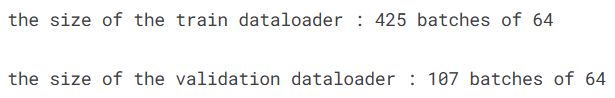
4.3数据可视化

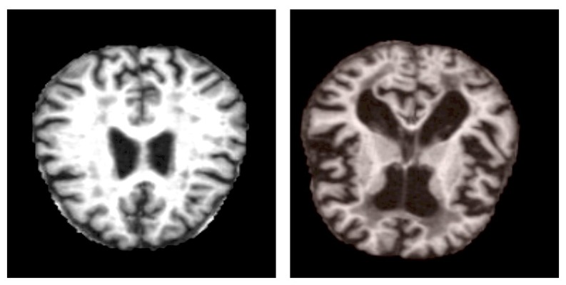
从验证数据集中随机抽取一批MRI图像样本进行可视化展示。对于阿尔茨海默病诊断研究,观察原始脑部MRI图像的质量和特征非常重要,这能帮助我们理解数据特点并检查预处理是否正确。
# 从验证数据集中获取一个批次的图像和标签样本
# iter()将数据集转换为迭代器,next()获取下一个批次
img_sample, label_sample = next(iter(val_set))

# 创建2行4列的子图网格,用于展示8个MRI图像样本
# figsize=(15, 10)设置整个图形大小为15x10英寸
fig, axis = plt.subplots(2, 4, figsize=(15, 10))

# 遍历所有子图(共8个),在每个子图中显示一张MRI图像
for i, ax in enumerate(axis.flat):
    # 将第i个图像样本从TensorFlow张量转换为numpy数组
    # 因为matplotlib的imshow函数需要numpy数组格式
    img = img_sample[i].numpy()

    # 在当前子图中显示MRI图像
    ax.imshow(img)

    # 关闭坐标轴显示,使图像更清晰
    # MRI医学图像通常不需要显示坐标刻度
    ax.axis('off')

    # 设置子图标题,显示对应的疾病类别名称
    # label_sample[i]是one-hot编码格式,使用argmax()找到值为1的位置索引
    # 通过label_map字典将数字索引转换为可读的类别名称
    ax.set(title=f"{label_map[np.array(label_sample[i]).argmax()]}")

# 显示完整图形
plt.show()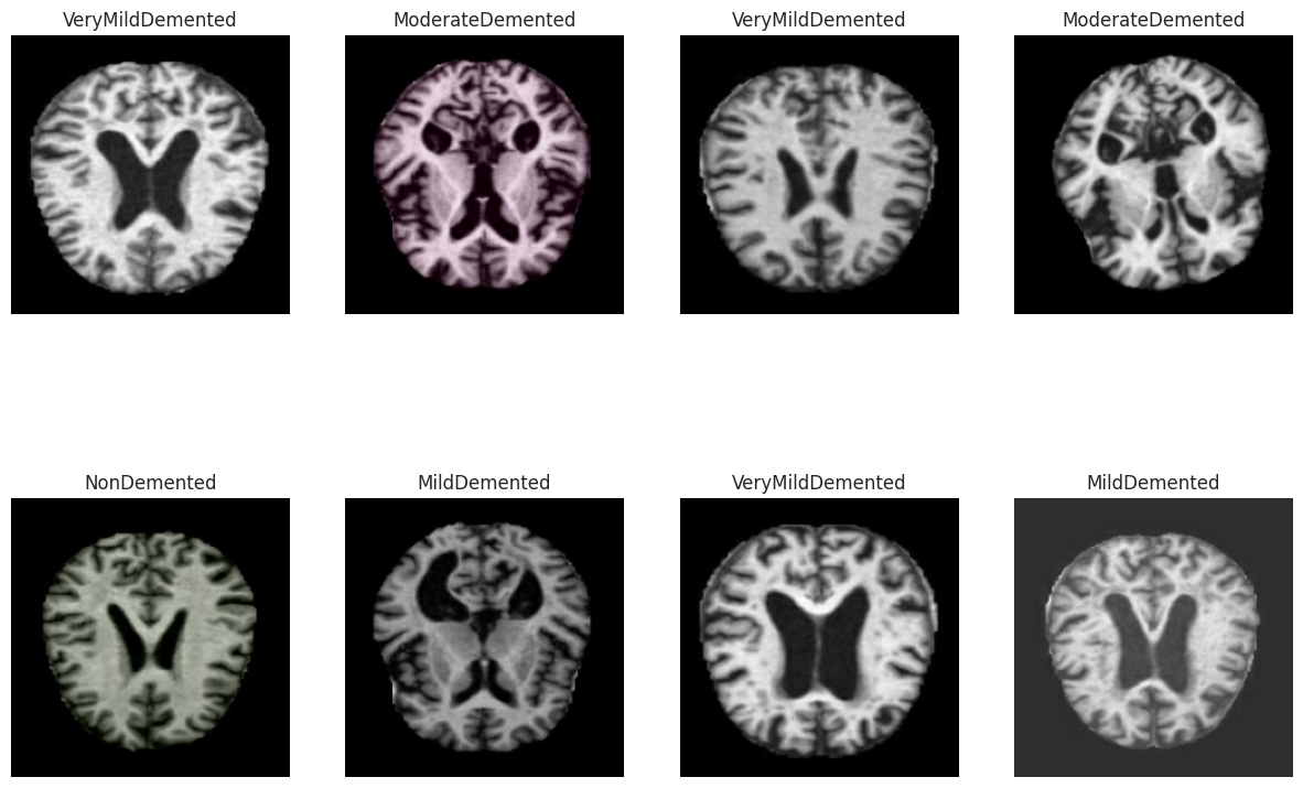
4.4构建模型
这里定义了基于Xception架构的阿尔茨海默病MRI图像识别模型。Xception是一种高效的卷积神经网络,采用深度可分离卷积设计,在保持较高精度的同时减少了参数数量,特别适合处理医学图像这类需要精细特征分析的任务。
# 加载预训练的Xception模型作为基础特征提取器
base_model = Xception(
    input_shape=(IMG_SIZE, IMG_SIZE, 3),  # 输入图像尺寸:224x224像素,RGB三通道
    include_top=False,                     # 不包含原始顶部分类层(我们将自定义分类头)
    weights='imagenet'                     # 使用在ImageNet数据集上预训练的权重
)

# 设置基础模型为可训练状态
# 在迁移学习中,通常先冻结预训练层,然后逐渐解冻进行微调
# 这里直接设置为可训练,将从头开始微调所有层
base_model.trainable = True

# 构建完整的序列模型
model = tf.keras.Sequential([
    # 基础模型:Xception特征提取器
    base_model,

    # 全局平均池化层:将特征图的空间维度(宽和高)压缩为1x1
    # 对每个特征通道的激活值进行平均,得到一个固定长度的特征向量
    # 相比展平层(Flatten),全局平均池化能减少参数数量并增强泛化能力
    tf.keras.layers.GlobalAveragePooling2D(),

    # 全连接层:256个神经元,使用ReLU激活函数
    # 这一层进一步组合和抽象特征,增强模型的非线性表达能力
    tf.keras.layers.Dense(256, activation='relu'),

    # 输出层:神经元数量等于类别数,使用Softmax激活函数
    # Softmax将输出转换为概率分布,每个类别的概率和为1
    tf.keras.layers.Dense(N_CLASSES, activation='softmax')
])

# 打印模型结构摘要
# 显示每层的输出形状、参数数量和总参数量
model.summary()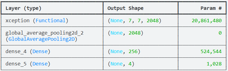
说明:模型采用迁移学习策略,使用在ImageNet上预训练的Xception模型作为特征提取器。Xception(Extreme Inception)是Inception架构的改进版本,通过深度可分离卷积替代标准卷积操作,显著减少了计算复杂度和参数量,同时保持了良好的特征提取能力,这对于处理医学图像中的细微结构变化特别有利。基础模型设置为可训练状态(trainable=True),这意味着在训练过程中不仅自定义的分类层会更新参数,预训练的Xception层也会进行微调。这种完全的微调策略通常需要较多的训练数据和计算资源,但可能获得更好的性能,因为模型可以根据阿尔茨海默病MRI图像的特点调整所有层次的特征表示。全局平均池化层是一个关键设计选择,它代替了传统的展平层。对于医学图像分类任务,全局平均池化有几个优势:首先,它显著减少了参数数量,降低了过拟合风险;其次,它对输入图像的空间平移具有更好的不变性;第三,它为模型提供了一定的解释性,因为每个特征通道对应一个特定的特征检测器。全连接层包含256个神经元,这是一个适中的维度,既提供了足够的表达能力,又避免了过大的参数量。输出层使用Softmax激活函数,为每个阿尔茨海默病类别生成概率分布。
4.5训练模型
这块我们配置了模型训练的各种组件并启动了训练过程。对于阿尔茨海默病诊断这种医学图像分析任务,我们需要采用稳健的训练策略和全面的监控指标,确保模型不仅准确率高,还要具备临床可解释性和可靠性。
def get_callbacks(model_name):
    """
    创建训练回调函数集合
    参数:
        model_name: 模型名称,用于保存文件命名
    返回:
        callbacks: 回调函数列表
    """
    callbacks = []  # 初始化回调函数列表

    # ------------------- 模型检查点回调 -------------------
    # 在训练过程中定期保存模型,特别是保存性能最好的模型
    checkpoint = ModelCheckpoint(
        filepath=f'model.{model_name}.h5',  # 模型保存路径和文件名
        verbose=1,                          # 显示保存信息
        monitor='val_accuracy',             # 监控验证准确率
        mode='max'                          # 模式为最大化(希望准确率越高越好)
    )
    callbacks.append(checkpoint)  # 添加到回调列表

    # ------------------- 学习率衰减回调 -------------------
    # 当模型性能停滞时自动降低学习率,帮助模型跳出局部最优
    reduce_lr = ReduceLROnPlateau(
        monitor='val_loss',       # 监控验证损失
        factor=0.2,               # 学习率衰减因子:每次降低80%(乘以0.2)
        patience=3,               # 等待3个epoch,如果验证损失没有改善则降低学习率
        min_lr=1e-6,              # 学习率的最小值,避免学习率过小导致训练停滞
        verbose=1                 # 显示学习率调整信息
    )
    callbacks.append(reduce_lr)

    # ------------------- 早停回调 -------------------
    # 当验证损失不再改善时提前停止训练,防止过拟合
    early_stopping = EarlyStopping(
        monitor='val_loss',           # 监控验证损失
        patience=5,                   # 容忍验证损失连续5个epoch没有改善
        restore_best_weights=True,    # 训练结束后恢复最佳模型权重(而不是最后一轮的权重)
        verbose=1                     # 显示早停信息
    )
    callbacks.append(early_stopping)

    return callbacks


# 定义损失函数
# 分类交叉熵损失:适用于多分类任务,与Softmax输出层配合使用
LOSS = tf.keras.losses.CategoricalCrossentropy()

# 定义优化器
# Adamax优化器:Adam的变体,对学习率变化更稳定
# learning_rate=0.001:初始学习率0.001
OPTIM = tf.keras.optimizers.Adamax(learning_rate=0.001)

# 定义评估指标
# 除了准确率,还计算精确率和召回率,这在医学诊断中特别重要
METRICS = [
    'accuracy',  # 准确率:正确分类的样本比例
    tf.keras.metrics.Precision(name='precision'),  # 精确率:预测为正的样本中实际为正的比例
    tf.keras.metrics.Recall(name='recall')         # 召回率:实际为正的样本中被正确预测的比例
]

# 获取回调函数
CALLBACKS = get_callbacks('Xception')

# 编译模型:配置训练过程
model.compile(loss=LOSS, optimizer=OPTIM, metrics=METRICS)

# 在GPU设备上执行训练(如果可用)
with tf.device("/GPU:0"):
    # 开始模型训练
    history = model.fit(
        train_set,           # 训练数据集
        epochs=EPOCHS,       # 训练轮数(之前定义为10)
        validation_data=val_set,  # 验证数据集
        callbacks=[CALLBACKS]     # 训练回调函数
    )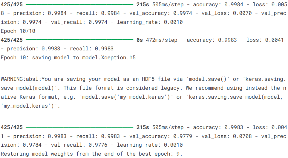
说明:回调函数的配置特别重要:模型检查点确保我们不会丢失训练过程中的最佳模型;学习率衰减允许模型在训练后期进行更精细的参数调整;早停机制防止模型在训练集上过度拟合。这些回调共同构成了一个智能的训练监控系统。损失函数选择分类交叉熵,这是多分类任务的标准选择。优化器使用Adamax,这是Adam优化器的一种变体,在某些任务上表现更稳定,对学习率的选择不那么敏感。评估指标不仅包括准确率,还特别加入了精确率和召回率,这对于医学诊断至关重要:高精确率意味着当模型预测患者有阿尔茨海默病时,误诊的可能性较低;高召回率意味着尽可能少地漏诊实际患者。在临床实践中,这两者的权衡需要根据具体应用场景决定。训练过程指定在GPU设备上执行,这能显著加速模型训练,特别是处理MRI图像这种较大的数据集时。训练历史记录在history对象中,包含了每个epoch的训练损失、验证损失、准确率、精确率和召回率等指标的变化情况,为后续的性能分析和可视化提供了完整数据。
4.6模型评估
首先输出模型在训练集上的最终性能指标,包括损失、准确率、精确率和召回率。
# 打印训练集的最终性能指标
# history.history包含了训练过程中每个epoch的指标记录
# [-1]获取最后一个epoch的值
print(f"The training loss is : {history.history['loss'][-1]:0.2f}\n")
print(f"The training accuracy is : {(history.history['accuracy'][-1]*100):0.2f}%\n")
print(f"The training precision is : {history.history['precision'][-1]:0.2f}\n")
print(f"The training recall is : {history.history['recall'][-1]:0.2f}\n")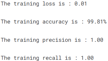
接着输出模型在验证集上的最终性能指标,验证集性能更能反映模型的泛化能力,因为这部分数据在训练过程中未被用于参数更新。
# 打印验证集的最终性能指标
print(f"The validation loss is : {history.history['val_loss'][-1]:0.2f}\n")
print(f"The validation accuracy is : {(history.history['val_accuracy'][-1]*100):0.2f}%\n")
print(f"The validation precision is : {history.history['val_precision'][-1]:0.2f}\n")
print(f"The validation recall is : {history.history['val_recall'][-1]:0.2f}\n")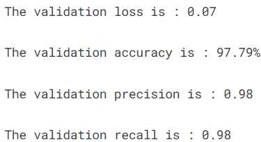
接着通过四个子图展示模型在整个训练过程中各项指标的变化趋势,帮助我们理解模型的学习动态和收敛情况。
# 创建2行2列的子图网格,用于展示四个训练指标的变化曲线
figure, axis = plt.subplots(2, 2, figsize=(15, 15))

# ------------------- 第一个子图:损失曲线 -------------------
axis[0, 0].plot(history.history['loss'], label='train')  # 训练损失曲线
axis[0, 0].plot(history.history['val_loss'], label='val')  # 验证损失曲线
axis[0, 0].set_title('Training/validation loss over Epochs', fontsize=20, fontweight='bold')
axis[0, 0].set_xlabel('Epochs')
axis[0, 0].set_ylabel('loss')
axis[0, 0].legend()

# ------------------- 第二个子图:准确率曲线 -------------------
axis[1, 0].plot(history.history['accuracy'], label='train')  # 训练准确率曲线
axis[1, 0].plot(history.history['val_accuracy'], label='val')  # 验证准确率曲线
axis[1, 0].set_title('Training/validation accuracy over Epochs')
axis[1, 0].set_xlabel('epoch')
axis[1, 0].set_ylabel('Accuracy')
axis[1, 0].legend()

# ------------------- 第三个子图:精确率曲线 -------------------
axis[0, 1].plot(history.history['precision'], label='train')  # 训练精确率曲线
axis[0, 1].plot(history.history['val_precision'], label='val')  # 验证精确率曲线
axis[0, 1].set_title('Training/validation precision over Epochs')
axis[0, 1].set_xlabel('epoch')
axis[0, 1].set_ylabel('Precision')
axis[0, 1].legend()

# ------------------- 第四个子图:召回率曲线 -------------------
axis[1, 1].plot(history.history['recall'], label='train')  # 训练召回率曲线
axis[1, 1].plot(history.history['val_recall'], label='val')  # 验证召回率曲线
axis[1, 1].set_title('Training/validation recall over Epochs')
axis[1, 1].set_xlabel('epoch')
axis[1, 1].set_ylabel('Recall')
axis[1, 1].legend()

plt.show()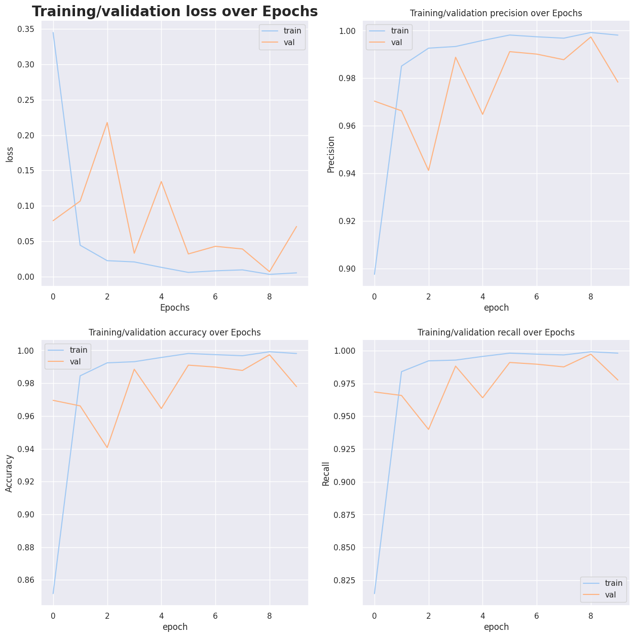
生成混淆矩阵,以可视化的方式展示模型在各个阿尔茨海默病类别上的具体表现,包括正确分类和混淆情况。
# 从验证集中获取一个批次的测试数据和标签
x_test, y_test = next(iter(val_set))

# 使用模型进行预测,并压缩维度
# round()函数将概率值四舍五入为0或1
y_preds = tf.squeeze(model.predict(x_test).round())

# 将one-hot编码的标签和预测结果转换为类别索引
y_test, y_preds = np.argmax(y_test, axis=1), np.argmax(y_preds, axis=1)

# 计算混淆矩阵
cm = confusion_matrix(y_test, y_preds)

# 将混淆矩阵转换为百分比形式,便于比较
cm_percent = cm / cm.sum() * 100

# 创建标签数组,同时显示原始数值和百分比
cm_labels = np.array([
    [f"{cm[i, j]}\n{cm_percent[i, j]:.2f}%" for j in range(cm.shape[1])]
    for i in range(cm.shape[0])
])

# 绘制混淆矩阵热力图
sns.heatmap(cm, annot=cm_labels, fmt='', cmap='YlOrBr')
plt.title('Alzheimer_Classifier Confusion Matrix')
plt.xlabel('Predicted')
plt.ylabel('Truth')
plt.show()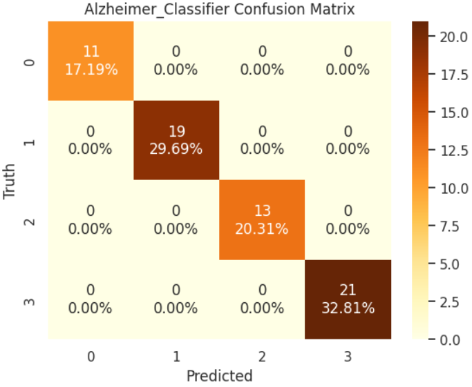
最后随机选择10个样本,展示模型的预测结果与真实标签的对比,直观了解模型在具体病例上的表现。
def predict(model, input, label):
    """
    随机抽样展示模型在具体样本上的预测结果
    参数:
        model: 训练好的模型
        input: 图像路径数组
        label: 对应标签数组
    """
    # 随机选择10个不同的样本索引(不重复)
    random_picks = np.random.choice(len(input), size=10, replace=False)

    # 获取选中的样本
    input_sample = input[random_picks]
    label_sample = label[random_picks]

    sample_imgs = []  # 存储处理后的图像
    sample_labels = []  # 存储对应的标签

    # 对每个选中的样本进行预处理
    for path, label in zip(input_sample, label_sample):
        img, lab = map_fn(path, label)  # 使用之前定义的预处理函数
        sample_imgs.append(img)
        sample_labels.append(lab)

    # 转换为numpy数组
    sample_imgs = np.array(sample_imgs)
    sample_labels = np.array(sample_labels)

    # 使用模型进行预测
    preds = tf.squeeze(model.predict(sample_imgs).round())

    # 创建2行5列的子图网格
    fig, axis = plt.subplots(2, 5, figsize=(25, 15))

    # 在每个子图中显示图像和预测结果
    for i, ax in enumerate(axis.flat):
        ax.imshow(sample_imgs[i])  # 显示MRI图像
        # 设置标题:显示预测类别和真实类别
        ax.set_title(
            f"Predicted : {label_map[np.array(preds[i]).argmax()]}\nTrue : {label_map[np.array(label_sample[i]).argmax()]}",
            fontsize=20
        )
        ax.axis('off')  # 关闭坐标轴

    plt.show()

# 在整个数据集上执行预测可视化
predict(model, dataset_paths, dataset_labels)
保存模型
model.save('Alzheimer_Classifier.keras')5.总结
本文基于Xception架构构建了阿尔茨海默病MRI图像识别模型,针对轻度痴呆、中度痴呆、非痴呆和极轻度痴呆四类脑部状态进行了系统研究。实验结果表明,模型在验证集上取得了97.79%的准确率,精确率和召回率均达到0.98,显示出优异的分类性能。通过迁移学习策略,利用ImageNet预训练的Xception模型进行特征提取,并结合全局平均池化与全连接层构建分类头,模型能够有效捕捉MRI图像中与阿尔茨海默病相关的脑结构变化特征。训练过程采用早停机制与学习率衰减策略,确保了模型的稳定收敛并避免了过拟合。混淆矩阵与随机样本可视化分析进一步验证了模型在不同痴呆程度间的区分能力,为阿尔茨海默病的早期筛查与辅助诊断提供了可行的深度学习解决方案,具有一定的临床参考价值。
源代码
import warnings
warnings.filterwarnings('ignore')
import pandas as pd
import numpy as np
import os
import glob as gb
import cv2
import matplotlib.pyplot as plt
import seaborn as sns
from sklearn.model_selection import train_test_split
from sklearn.metrics import confusion_matrix
import tensorflow as tf
from tensorflow.keras.applications import Xception
from tensorflow.keras.callbacks import EarlyStopping, ReduceLROnPlateau, ModelCheckpoint
sns.set_theme(style='darkgrid', palette='pastel')
color = sns.color_palette(palette='pastel')
gpus = tf.config.experimental.list_physical_devices('GPU')
DATASET_DIR = './augmented-alzheimer-mri-dataset/AugmentedAlzheimerDataset'
IMG_SIZE = 224
BATCH_SIZE = 64
BUFFER_SIZE = 1000
EPOCHS = 10
def ReadDataset(data_dir) :
    img_paths = []
    labels = []
    label_map = {}
    for idx , folder in enumerate(os.listdir(data_dir)) :
        label_map[idx] = folder
        for path in os.listdir(data_dir + '/' + folder) :
            files = gb.glob(pathname = str(data_dir + '/' + folder + '/' + path))
            for file in files :
                img_paths.append(file)
                labels.append(idx)

    return np.array(img_paths) , np.array(labels) , label_map

dataset_paths , dataset_labels , label_map = ReadDataset(DATASET_DIR)
N_CLASSES = len(label_map.keys())
print (" Shape before one-hot encoding : ", dataset_labels.shape)
dataset_labels= tf.keras.utils.to_categorical(dataset_labels,N_CLASSES)
print (" Shape after one-hot encoding : ", dataset_labels.shape)
train_data , val_data , train_labels , val_labels = train_test_split(dataset_paths , dataset_labels , train_size = 0.8 , random_state = 42)
def map_fn(img_path , label) :
    img = tf.io.read_file(img_path)
    img = tf.image.decode_jpeg(img)
    img = tf.image.resize(img , (IMG_SIZE , IMG_SIZE))
    img = tf.cast(img , tf.float32) / 255.

    return img , label

train_set = tf.data.Dataset.from_tensor_slices((train_data , train_labels))
train_set = train_set.map(map_fn)
train_set = train_set.shuffle(BUFFER_SIZE).batch(BATCH_SIZE)

val_set = tf.data.Dataset.from_tensor_slices((val_data , val_labels))
val_set = val_set.map(map_fn)
val_set = val_set.batch(BATCH_SIZE)
print(f"the size of the train dataloader : {len(train_set)} batches of {BATCH_SIZE}\n")
print(f"the size of the validation dataloader : {len(val_set)} batches of {BATCH_SIZE}\n")
img_sample , label_sample = next(iter(val_set))
fig , axis = plt.subplots(2 , 4 , figsize = (15 , 10))
for i , ax in enumerate(axis.flat) :
    img = img_sample[i].numpy()
    ax.imshow(img)
    ax.axis('off')
    ax.set(title = f"{label_map[np.array(label_sample[i]).argmax()]}")
plt.show()
base_model = Xception(
    input_shape = (IMG_SIZE , IMG_SIZE , 3) ,
    include_top = False ,
    weights = 'imagenet'
)

base_model.trainable = True
model = tf.keras.Sequential([
    base_model ,
    tf.keras.layers.GlobalAveragePooling2D() ,
    tf.keras.layers.Dense(256 , activation = 'relu') ,
    tf.keras.layers.Dense(N_CLASSES , activation = 'softmax')
])
model.summary()
def get_callbacks(model_name):
    callbacks = []

    checkpoint = ModelCheckpoint(filepath=f'model.{model_name}.h5', verbose=1, monitor='val_accuracy', mode='max')
    callbacks.append(checkpoint)

    reduce_lr = ReduceLROnPlateau(monitor='val_loss', factor=0.2, patience=3, min_lr=1e-6, verbose=1)
    callbacks.append(reduce_lr)

    early_stopping = EarlyStopping(monitor='val_loss', patience=5, restore_best_weights=True, verbose=1)
    callbacks.append(early_stopping)

    return callbacks

LOSS = tf.keras.losses.CategoricalCrossentropy()
OPTIM = tf.keras.optimizers.Adamax(learning_rate=0.001)
METRICS = [
    'accuracy' ,
    tf.keras.metrics.Precision(name = 'precision') ,
    tf.keras.metrics.Recall(name = 'recall')
]
CALLBACKS = get_callbacks('Xception')
model.compile(loss=LOSS , optimizer = OPTIM , metrics=METRICS )
with tf.device("/GPU:0") :
    history = model.fit(
        train_set ,
        epochs=EPOCHS ,
        validation_data=val_set ,
        callbacks = [CALLBACKS]
    )
print(f"The training loss is : {history.history['loss'][-1]:0.2f}\n")
print(f"The training accuracy is : {(history.history['accuracy'][-1]*100):0.2f}%\n")
print(f"The training precision is : {history.history['precision'][-1]:0.2f}\n")
print(f"The training recall is : {history.history['recall'][-1]:0.2f}\n")
print(f"The validation loss is : {history.history['val_loss'][-1]:0.2f}\n")
print(f"The validation accuracy is : {(history.history['val_accuracy'][-1]*100):0.2f}%\n")
print(f"The validation precision is : {history.history['val_precision'][-1]:0.2f}\n")
print(f"The validation recall is : {history.history['val_recall'][-1]:0.2f}\n")
figure , axis = plt.subplots(2,2,figsize=(15,15))


axis[0,0].plot(history.history['loss'] , label='train')
axis[0,0].plot(history.history['val_loss'] , label='val')
axis[0,0].set_title('Training/validation loss over Epochs' , fontsize = 20 , fontweight = 'bold')
axis[0,0].set_xlabel('Epochs')
axis[0,0].set_ylabel('loss')
axis[0,0].legend()


axis[1,0].plot(history.history['accuracy'], label='train')
axis[1,0].plot(history.history['val_accuracy'], label='val')
axis[1,0].set_title('Training/validation accuracy over Epochs')
axis[1,0].set_xlabel('epoch')
axis[1,0].set_ylabel('Accuracy')
axis[1,0].legend()


axis[0,1].plot(history.history['precision'], label='train')
axis[0,1].plot(history.history['val_precision'], label='val')
axis[0,1].set_title('Training/validation precision over Epochs')
axis[0,1].set_xlabel('epoch')
axis[0,1].set_ylabel('Precision')
axis[0,1].legend()


axis[1,1].plot(history.history['recall'], label='train')
axis[1,1].plot(history.history['val_recall'], label='val')
axis[1,1].set_title('Training/validation recall over Epochs')
axis[1,1].set_xlabel('epoch')
axis[1,1].set_ylabel('Recall')
axis[1,1].legend()
plt.show()
x_test , y_test = next(iter(val_set))
y_preds = tf.squeeze(model.predict(x_test).round())
y_test , y_preds = np.argmax(y_test , axis = 1) , np.argmax(y_preds , axis = 1)
cm = confusion_matrix(y_test,y_preds)
cm_percent = cm / cm.sum() * 100

cm_labels = np.array([
    [f"{cm[i, j]}\n{cm_percent[i, j]:.2f}%" for j in range(cm.shape[1])]
    for i in range(cm.shape[0])
])

sns.heatmap(cm,annot = cm_labels,fmt ='', cmap = 'YlOrBr')
plt.title('Alzheimer_Classifier Confusion Matrix')
plt.xlabel('Predicted')
plt.ylabel('Truth')
plt.show()
def predict(model , input , label) :
    random_picks = np.random.choice(len(input) , size = 10 , replace = False)

    input_sample = input[random_picks]
    label_sample = label[random_picks]

    sample_imgs = []
    sample_labels = []

    for path , label in zip(input_sample , label_sample) :
        img , lab = map_fn(path , label)
        sample_imgs.append(img)
        sample_labels.append(lab)

    sample_imgs = np.array(sample_imgs)
    sample_labels = np.array(sample_labels)

    preds = tf.squeeze(model.predict(sample_imgs).round())

    fig, axis = plt.subplots(2, 5, figsize=(25, 15))
    for i, ax in enumerate(axis.flat):
        ax.imshow(sample_imgs[i])
        ax.set_title(f"Predicted : {label_map[np.array(preds[i]).argmax()]}\nTrue : {label_map[np.array(label_sample[i]).argmax()]}" , fontsize = 20)
        ax.axis('off')
    plt.show()

predict(model , dataset_paths , dataset_labels)
model.save('Alzheimer_Classifier.keras')
资料获取,更多粉丝福利,关注下方公众号获取


AtomGit 是由开放原子开源基金会联合 CSDN 等生态伙伴共同推出的新一代开源与人工智能协作平台。平台坚持“开放、中立、公益”的理念,把代码托管、模型共享、数据集托管、智能体开发体验和算力服务整合在一起,为开发者提供从开发、训练到部署的一站式体验。
更多推荐


 14
14 0
0- 0


 已为社区贡献5条内容

所有评论(0)