电磁场仿真-主题091-神经形态光子学

kkchenjj

31人浏览 · 2026-03-26 22:57:43

kkchenjj · 2026-03-26 22:57:43 发布

主题091: 神经形态光子学 - 光子神经网络与计算

引言

神经形态光子学(Neuromorphic Photonics)是神经形态计算与光子学的交叉领域，旨在利用光的物理特性实现高效、高速、低功耗的类脑计算。与传统的电子神经形态芯片相比，光子神经形态系统具有以下独特优势：

超高带宽：光载波频率可达数百THz，支持超高速信号处理
低延迟：光速传播，延迟极低
低串扰：不同波长的光信号可在同一波导中传输而不相互干扰
并行处理：波分复用(WDM)技术支持大规模并行计算
低功耗：光信号传输损耗低，无需频繁信号再生

本教程将系统介绍神经形态光子学的核心概念、物理机制和实现方法，并通过Python仿真展示光子神经网络的构建和训练。

在这里插入图片描述

神经形态计算基础

2.1 生物神经元与突触

生物神经网络由神经元和突触组成：

2.1.1 神经元结构

胞体(Soma)：处理输入信号
树突(Dendrite)：接收来自其他神经元的信号
轴突(Axon)：输出信号到其他神经元
突触(Synapse)：神经元间的连接点

2.1.2 神经信号传递

树突接收神经递质，产生突触后电位(PSP)
PSP在胞体累加，形成膜电位
当膜电位超过阈值时，产生动作电位(脉冲)
脉冲沿轴突传播，通过突触传递到其他神经元

2.2 脉冲神经网络(SNN)

脉冲神经网络是第三代神经网络，使用离散的脉冲事件而非连续值进行信息编码：

2.2.1 信息编码方式

速率编码：脉冲发放频率表示信号强度
时间编码：脉冲的精确时间携带信息
群体编码：多个神经元的联合活动表示信息

2.2.2 神经元模型

漏积分发放(LIF)模型：

$τmdVdt=−(V−Vrest)+RI(t)\tau_m \frac{dV}{dt} = -(V - V_{rest}) + RI(t)$

当 $\geq V_{th}$ 时，发放脉冲并重置 $V = V_{reset}$

2.3 突触可塑性

突触权重可根据神经活动动态调整，这是学习和记忆的基础：

2.3.1 Hebbian学习规则

“一起激发的神经元连在一起”：

$Δwij∝xixj\Delta w_{ij} \propto x_i x_j$

2.3.2 脉冲时序依赖可塑性(STDP)

突触权重变化取决于前后神经元脉冲的时间差：

$Δt<0\Delta w = \begin{cases} A_+ e^{-\Delta t/\tau_+} & \text{if } \Delta t > 0 \\ -A_- e^{\Delta t/\tau_-} & \text{if } \Delta t < 0 \end{cases}$

其中 $Δt=tpost−tpre\Delta t = t_{post} - t_{pre}$

光子神经元模型

3.1 光子神经元实现方案

3.1.1 基于激光器的神经元

利用半导体激光器的增益开关特性：

VCSEL (垂直腔面发射激光器)
DFB激光器 (分布反馈激光器)
微环激光器

激光器速率方程：

$dndt=IqV−nτc−vgg(n)S\frac{dn}{dt} = \frac{I}{qV} - \frac{n}{\tau_c} - v_g g(n)S$

$dSdt=Γvgg(n)S−Sτp+βnτc\frac{dS}{dt} = \Gamma v_g g(n)S - \frac{S}{\tau_p} + \beta \frac{n}{\tau_c}$

其中：

$n$ ：载流子密度
$S$ ：光子密度
$I$ ：注入电流
$g (n)$ ：增益系数
$τc\tau_c$ , $τp\tau_p$ ：载流子和光子寿命

3.1.2 基于微环谐振器的神经元

利用光学双稳态实现类神经元响应：

$Pout=Pin1+(2Qω0(ω−ω0)−γPin)2P_{out} = \frac{P_{in}}{1 + \left(\frac{2Q}{\omega_0}(\omega - \omega_0) - \gamma P_{in}\right)^2}$

其中 $γ\gamma$ 是非线性系数。

3.2 光子神经元特性

3.2.1 发放阈值

光子神经元的阈值由激光器的阈值电流或谐振器的双稳态阈值决定。

3.2.2 不应期

绝对不应期：激光器载流子恢复时间
相对不应期：增益恢复过程

3.2.3 发放频率

最大发放频率受限于：

$fmax≈1τcarrier+τphotonf_{max} \approx \frac{1}{\tau_{carrier} + \tau_{photon}}$

对于VCSEL，可达数十GHz。

3.3 级联与网络

光子神经元可通过光波导级联：

直接耦合：通过波导连接
间接耦合：通过谐振器耦合
波长路由：利用WDM实现全连接

光学突触与权重调制

4.1 光学权重实现

4.1.1 MZI (马赫-曾德尔干涉仪)

MZI是最常用的光学权重实现方案：

透射率：

$\cos^2\left(\frac{\Delta\phi}{2}\right)$

通过热光或电光效应调节相位差 $Δϕ\Delta\phi$ 。

4.1.2 微环权重库

使用微环谐振器阵列实现可编程权重：

$T(λ)=τ2−2τcos⁡(ϕ)+11−2τcos⁡(ϕ)+τ2T(\lambda) = \frac{\tau^2 - 2\tau\cos(\phi) + 1}{1 - 2\tau\cos(\phi) + \tau^2}$

其中 $τ\tau$ 是耦合系数， $ϕ\phi$ 是往返相位。

4.1.3 相变材料

利用Ge₂Sb₂Te₅(GST)等相变材料实现非易失性权重存储：

晶态：高折射率，低透射
非晶态：低折射率，高透射

4.2 权重矩阵实现

4.2.1 MZI网格

使用三角网格实现任意酉矩阵：

$\prod_{i<j} T_{ij}$

其中 $T_{ij}$ 是基本MZI单元， $D$ 是对角相位矩阵。

4.2.2 波分复用权重库

不同波长对应不同权重，实现大规模并行计算。

4.3 光学STDP实现

4.3.1 基于光脉冲的STDP

利用光脉冲的时间重叠实现权重更新：

前脉冲和后脉冲在光波导中传播
脉冲重叠产生干涉
干涉结果决定权重变化方向

4.3.2 基于光电效应的STDP

使用光电导材料：

$ΔG∝∫Ipre(t)Ipost(t)dt\Delta G \propto \int I_{pre}(t) I_{post}(t) dt$

光子脉冲神经网络

5.1 网络架构

5.1.1 全连接层

使用光学权重库实现：

$yi=f(∑jWijxj+bi)y_i = f\left(\sum_j W_{ij} x_j + b_i\right)$

其中 $f$ 是光子神经元激活函数。

5.1.2 脉冲传播

光脉冲在波导中传播：

时间延迟：由波导长度决定
衰减：由波导损耗决定
色散：由波导色散特性决定

5.2 训练方法

5.2.1 无监督学习

STDP训练：

对于每个训练样本:
    前向传播产生脉冲序列
    根据脉冲时间差更新权重
    权重更新: Δw = f(Δt)

5.2.2 监督学习

基于梯度的训练：

使用替代梯度(Surrogate Gradient)解决脉冲不可微问题
时间反向传播(BPTT)

5.3 网络性能

5.3.1 分类精度

在MNIST等基准数据集上，光子SNN可达到：

简单网络：~95% 精度
深度网络：~99% 精度

5.3.2 能效比

光子SNN的能效可达：

10-100 TOPS/W (理论值)
比电子实现高2-3个数量级

光子储备池计算

6.1 储备池计算原理

储备池计算(RC)是一种特殊的循环神经网络架构：

6.1.1 基本结构

输入层：固定权重映射到储备池
储备池：大规模随机连接的循环网络
读出层：线性可训练权重

6.1.2 状态更新

$(1-\alpha)x(t) + \alpha f(W_{res} x(t) + W_{in} u(t))$

其中 $α\alpha$ 是泄漏率。

6.2 光子储备池实现

6.2.1 延迟线储备池

使用光纤延迟线实现时间序列处理：

输入信号调制光载波
在光纤环中传播产生延迟
不同抽头对应不同时间步

6.2.2 光学非线性

储备池需要非线性激活：

电光调制器：sin²非线性
半导体光放大器(SOA)：饱和非线性
克尔效应：光学非线性

6.3 应用场景

6.3.1 时间序列预测

混沌系统预测
金融时间序列
语音识别

6.3.2 记忆容量

储备池的记忆容量：

$\sum_{\tau=1}^{\infty} MC_\tau$

其中 $MCτMC_\tau$ 是延迟 $τ\tau$ 的记忆容量。

光子卷积神经网络

7.1 光学卷积实现

7.1.1 4F系统

使用傅里叶光学实现卷积：

$\mathcal{F}^{-1}\{\mathcal{F}\{f(x,y)\} \cdot \mathcal{F}\{h(x,y)\}\}$

其中：

第一个透镜：傅里叶变换
频域滤波：乘法运算
第二个透镜：逆傅里叶变换

7.1.2 空间光调制器(SLM)

SLM实现可编程卷积核：

相位型SLM：纯相位调制
振幅型SLM：振幅调制
复数型SLM：振幅和相位联合调制

7.2 光子CNN架构

7.2.1 卷积层

使用光学4F系统实现：

输入图像 → 透镜1 → SLM(卷积核) → 透镜2 → 输出特征图

7.2.2 池化层

光学池化实现：

平均池化：使用微透镜阵列
最大池化：使用 Winner-take-all 电路

7.2.3 全连接层

使用光学权重库实现矩阵乘法。

7.3 性能优势

7.3.1 处理速度

光子CNN的处理速度：

帧率：可达MHz甚至GHz
延迟：纳秒级

7.3.2 能效

相比电子CNN：

能效提升：10-1000倍
特别适合大规模图像处理

全光神经网络推理

8.1 衍射神经网络

8.1.1 衍射光学元件(DOE)

使用相位掩模实现神经网络层：

$Eout(x,y)=Ein(x,y)⋅eiϕ(x,y)E_{out}(x,y) = E_{in}(x,y) \cdot e^{i\phi(x,y)}$

其中 $ϕ(x,y)\phi(x,y)$ 是相位掩模。

8.1.2 角谱传播

光场在自由空间传播：

$\mathcal{F}^{-1}\{E(0) \cdot H(f_x, f_y)\}$

传播核：

$e^{ikz\sqrt{1 - (\lambda f_x)^2 - (\lambda f_y)^2}}$

8.2 多层衍射网络

8.2.1 网络结构

输入光场 → 相位掩模1 → 传播 → 相位掩模2 → ... → 输出

8.2.2 训练方法

使用误差反向传播训练相位掩模：

$∂L∂ϕ=∂L∂E⋅∂E∂ϕ\frac{\partial L}{\partial \phi} = \frac{\partial L}{\partial E} \cdot \frac{\partial E}{\partial \phi}$

8.3 应用

8.3.1 图像分类

MNIST：>90% 准确率
CIFAR-10：>70% 准确率

8.3.2 其他应用

目标检测
语义分割
图像重建

光子神经形态芯片架构

9.1 芯片设计

9.1.1 核心架构

多核心设计：

每个核心包含多个光子神经元
核心内全连接
核心间稀疏连接

9.1.2 互连网络

波导互连：片上波导
WDM互连：波分复用
自由空间互连：3D封装

9.2 关键器件

9.2.1 激光器阵列

VCSEL阵列：850nm或980nm
硅光集成激光器：1550nm

9.2.2 调制器

MZI调制器：高速调制
微环调制器：紧凑设计
电吸收调制器：高效率

9.2.3 探测器

光电二极管：高速响应
超导纳米线探测器：单光子灵敏度

9.3 性能指标

9.3.1 计算密度

神经元密度：1000-10000 neurons/mm²
突触密度：100000-1000000 synapses/mm²

9.3.2 能效

目标能效：>10 TOPS/W
当前水平：0.1-1 TOPS/W

9.3.3 延迟

片上延迟：<1 ns
片间延迟：<10 ns

Python仿真实现

10.1 光子神经元

class PhotonicNeuron:
    """光子神经元模型"""
    
    def __init__(self, tau_mem=1e-9, tau_syn=0.5e-9, V_th=1.0):
        self.tau_mem = tau_mem
        self.tau_syn = tau_syn
        self.V_th = V_th
        self.V = 0.0
        self.I_syn = 0.0
        
    def update(self, I_input, dt, t):
        """更新神经元状态"""
        # 突触电流动力学
        dI_syn = (-self.I_syn / self.tau_syn + I_input) * dt
        self.I_syn += dI_syn
        
        # 膜电位动力学
        dV = (-self.V / self.tau_mem + self.I_syn) * dt
        self.V += dV
        
        # 检查发放
        if self.V >= self.V_th:
            self.V = 0.0
            return 1.0
        return 0.0

10.2 光学突触

class OpticalSynapse:
    """光学突触 - MZI实现"""
    
    def __init__(self, weight=0.5):
        self.weight = weight
        self.phase_shift = np.arccos(np.sqrt((weight + 1) / 2))
        
    def mzi_transmission(self):
        """MZI透射率"""
        return np.cos(self.phase_shift / 2) ** 2
    
    def apply(self, optical_input):
        """应用突触权重"""
        transmission = self.mzi_transmission()
        return optical_input * transmission * self.weight

10.3 储备池计算

class PhotonicReservoir:
    """光子储备池"""
    
    def __init__(self, n_nodes=100, spectral_radius=0.9):
        self.n_nodes = n_nodes
        self.W_res = np.random.randn(n_nodes, n_nodes)
        eigenvalues = np.abs(eig(self.W_res)[0])
        self.W_res *= spectral_radius / np.max(eigenvalues)
        self.state = np.zeros(n_nodes)
        
    def update(self, u):
        """更新储备池状态"""
        activation = np.tanh(self.W_res @ self.state + u)
        self.state = (1 - 0.3) * self.state + 0.3 * activation
        return self.state

总结与展望

11.1 技术总结

本教程系统介绍了神经形态光子学的核心内容：

光子神经元：基于激光器和微环谐振器的实现
光学突触：MZI和相变材料权重调制
脉冲神经网络：光域SNN架构和训练
储备池计算：延迟线储备池和记忆容量
卷积神经网络：4F光学系统和SLM实现
全光神经网络：衍射神经网络和相位掩模
芯片架构：多核心设计和WDM互连

11.2 发展趋势

神经形态光子学的发展趋势：

集成度提升：从分立器件到大规模集成
性能优化：更高速度、更低功耗
算法创新：适合光子实现的专用算法
应用拓展：从图像处理到决策控制
异构集成：光电混合系统

11.3 挑战与机遇

11.3.1 技术挑战

非线性实现：光学非线性较弱
可扩展性：大规模集成困难
训练算法：光域训练机制不完善
封装测试：光电混合封装复杂

11.3.2 发展机遇

AI应用爆发：边缘计算需求增长
硅光技术成熟：CMOS兼容工艺
新材料涌现：二维材料、相变材料
算法硬件协同：软硬件联合优化

11.4 学习建议

学习神经形态光子学需要掌握：

光学基础：波动光学、傅里叶光学
光子器件：波导、谐振器、调制器
神经科学：神经元模型、突触可塑性
机器学习：神经网络、优化算法
集成电路：硅光工艺、封装测试

通过理论学习和Python仿真相结合，可以深入理解神经形态光子学的工作原理和设计方法，为参与这一前沿领域打下坚实基础。

"""
主题091: 神经形态光子学 - 光子神经网络与计算
Neuromorphic Photonics - Photonic Neural Networks and Computing

本程序实现神经形态光子学的核心仿真，包括：
1. 光子神经元模型 (Photonic Neuron)
2. 光学突触与权重调制 (Optical Synapse)
3. 光子脉冲神经网络 (Spiking Neural Network)
4. 光子储备池计算 (Reservoir Computing)
5. 光子卷积神经网络 (Photonic CNN)
6. 全光神经网络推理 (All-optical Inference)
7. 光子神经形态芯片架构 (Photonic Neuromorphic Architecture)
"""

import numpy as np
import matplotlib.pyplot as plt
from scipy.integrate import odeint, solve_ivp
from scipy.linalg import expm, eig
from scipy.signal import convolve2d
from scipy.ndimage import gaussian_filter
import matplotlib
matplotlib.use('Agg')
plt.rcParams['font.sans-serif'] = ['SimHei', 'DejaVu Sans']
plt.rcParams['axes.unicode_minus'] = False

# 物理常数
c = 299792458  # 光速 (m/s)
h = 6.626e-34  # 普朗克常数 (J·s)
hbar = h / (2 * np.pi)
e = 1.602e-19  # 元电荷 (C)
k_B = 1.381e-23  # 玻尔兹曼常数 (J/K)

print("=" * 60)
print("主题091: 神经形态光子学 - 光子神经网络与计算")
print("=" * 60)

# ============================================================
# 1. 光子神经元模型
# ============================================================

class PhotonicNeuron:
    """
    光子神经元模型 - 基于光学谐振腔的非线性动力学
    
    使用半导体激光器或微环谐振器实现类神经元响应
    """
    
    def __init__(self, tau_mem=1e-9, tau_syn=0.5e-9, V_th=1.0, 
                 refractory_period=2e-9, wavelength=1550e-9):
        """
        参数:
            tau_mem: 膜时间常数 (s)
            tau_syn: 突触时间常数 (s)
            V_th: 发放阈值
            refractory_period: 不应期 (s)
            wavelength: 工作波长 (m)
        """
        self.tau_mem = tau_mem
        self.tau_syn = tau_syn
        self.V_th = V_th
        self.refractory_period = refractory_period
        self.wavelength = wavelength
        
        # 神经元状态
        self.V = 0.0  # 膜电位
        self.I_syn = 0.0  # 突触电流
        self.last_spike_time = -np.inf  # 上次发放时间
        self.spike_times = []  # 发放时间记录
        
        # 光学参数
        self.n_eff = 3.5  # 有效折射率
        self.alpha_loss = 100  # 损耗系数 (1/m)
        
    def reset(self):
        """重置神经元状态"""
        self.V = 0.0
        self.I_syn = 0.0
        self.last_spike_time = -np.inf
        self.spike_times = []
        
    def update(self, I_input, dt, t):
        """
        更新神经元状态
        
        参数:
            I_input: 输入电流
            dt: 时间步长
            t: 当前时间
        """
        # 检查不应期
        if t - self.last_spike_time < self.refractory_period:
            self.V = 0.0
            return 0.0
        
        # 突触电流动力学 (指数衰减)
        dI_syn = (-self.I_syn / self.tau_syn + I_input) * dt
        self.I_syn += dI_syn
        
        # 膜电位动力学 (漏积分发放模型)
        dV = (-self.V / self.tau_mem + self.I_syn) * dt
        self.V += dV
        
        # 检查发放
        if self.V >= self.V_th:
            self.V = 0.0
            self.last_spike_time = t
            self.spike_times.append(t)
            return 1.0  # 发放脉冲
        
        return 0.0
    
    def simulate(self, I_inputs, dt, t_max):
        """
        仿真神经元响应
        
        参数:
            I_inputs: 输入电流数组
            dt: 时间步长
            t_max: 最大仿真时间
        """
        self.reset()
        n_steps = int(t_max / dt)
        t_array = np.linspace(0, t_max, n_steps)
        
        V_trace = np.zeros(n_steps)
        spikes = np.zeros(n_steps)
        
        for i in range(n_steps):
            V_trace[i] = self.V
            spikes[i] = self.update(I_inputs[i], dt, t_array[i])
        
        return t_array, V_trace, spikes
    
    def f_i_curve(self, I_range):
        """
        计算f-I曲线 (输入-输出频率关系)
        
        参数:
            I_range: 输入电流范围
        """
        frequencies = []
        
        for I_const in I_range:
            self.reset()
            dt = 0.1e-9
            t_max = 100e-9
            n_steps = int(t_max / dt)
            
            for i in range(n_steps):
                t = i * dt
                self.update(I_const, dt, t)
            
            freq = len(self.spike_times) / t_max
            frequencies.append(freq)
        
        return np.array(frequencies)


class VCSELNeuron(PhotonicNeuron):
    """
    VCSEL (垂直腔面发射激光器) 神经元
    
    基于激光器的增益开关特性实现脉冲发放
    """
    
    def __init__(self, tau_mem=1e-9, tau_syn=0.5e-9, V_th=1.0,
                 refractory_period=2e-9, wavelength=850e-9,
                 P_threshold=1e-3, tau_photon=1e-12):
        super().__init__(tau_mem, tau_syn, V_th, refractory_period, wavelength)
        
        self.P_threshold = P_threshold  # 激光阈值功率 (W)
        self.tau_photon = tau_photon  # 光子寿命 (s)
        self.carrier_density = 0.0  # 载流子密度
        self.photon_density = 0.0  # 光子密度
        
    def laser_rate_equations(self, y, t, I_pump):
        """
        激光器速率方程
        
        dn/dt = I/qV - n/tau - v_g*g(n)*S
        dS/dt = Gamma*v_g*g(n)*S - S/tau_p + beta*n/tau
        """
        n, S = y
        
        # 参数
        tau_carrier = 1e-9  # 载流子寿命
        v_g = c / self.n_eff  # 群速度
        g_0 = 1e-12  # 增益系数
        n_tr = 1e18  # 透明载流子密度
        Gamma = 0.1  # 限制因子
        beta = 1e-4  # 自发辐射因子
        
        # 增益
        g = g_0 * np.log(n / n_tr) if n > n_tr else 0
        
        # 速率方程
        dn_dt = I_pump - n / tau_carrier - v_g * g * S
        dS_dt = Gamma * v_g * g * S - S / self.tau_photon + beta * n / tau_carrier
        
        return [dn_dt, dS_dt]
    
    def update_laser(self, I_pump, dt):
        """更新激光器状态"""
        y0 = [self.carrier_density, self.photon_density]
        t_span = [0, dt]
        
        sol = solve_ivp(lambda t, y: self.laser_rate_equations(y, t, I_pump),
                       t_span, y0, method='RK45')
        
        self.carrier_density = sol.y[0, -1]
        self.photon_density = sol.y[1, -1]
        
        # 检测脉冲发放
        spike = 1.0 if self.photon_density > self.P_threshold else 0.0
        
        return spike


# ============================================================
# 2. 光学突触与权重调制
# ============================================================

class OpticalSynapse:
    """
    光学突触 - 实现可编程光权重
    
    使用MZI (Mach-Zehnder Interferometer) 或微环谐振器
    """
    
    def __init__(self, weight=0.5, weight_range=(-1, 1), 
                 modulation_speed=10e9, wavelength=1550e-9):
        """
        参数:
            weight: 初始权重
            weight_range: 权重范围
            modulation_speed: 调制速度 (Hz)
            wavelength: 工作波长
        """
        self.weight = weight
        self.weight_range = weight_range
        self.modulation_speed = modulation_speed
        self.wavelength = wavelength
        
        # MZI参数
        self.phase_shift = np.arccos(np.sqrt((weight + 1) / 2))
        
    def set_weight(self, weight):
        """设置权重"""
        self.weight = np.clip(weight, *self.weight_range)
        # 映射到相位
        self.phase_shift = np.arccos(np.sqrt((self.weight + 1) / 2))
        
    def mzi_transmission(self, phase_diff=None):
        """
        计算MZI透射率
        
        T = cos²(Δφ/2)
        """
        if phase_diff is None:
            phase_diff = self.phase_shift
        
        T = np.cos(phase_diff / 2) ** 2
        return T
    
    def apply(self, optical_input):
        """
        应用突触权重到光输入
        
        参数:
            optical_input: 输入光场 (复数或实数振幅)
        """
        transmission = self.mzi_transmission()
        return optical_input * transmission * self.weight
    
    def update_weight_stdp(self, delta_t, A_plus=0.1, A_minus=0.1, 
                          tau_plus=20e-3, tau_minus=20e-3):
        """
        STDP (脉冲时序依赖可塑性) 权重更新
        
        参数:
            delta_t: 前后神经元发放时间差 (t_post - t_pre)
            A_plus: 增强幅度
            A_minus: 抑制幅度
            tau_plus, tau_minus: 时间常数
        """
        if delta_t > 0:
            # 前神经元先发放 -> 增强
            delta_w = A_plus * np.exp(-delta_t / tau_plus)
        else:
            # 后神经元先发放 -> 抑制
            delta_w = -A_minus * np.exp(delta_t / tau_minus)
        
        self.set_weight(self.weight + delta_w)
        return delta_w


class PhotonicWeightBank:
    """
    光子权重库 - 实现权重矩阵
    
    使用MZI网格或微环阵列
    """
    
    def __init__(self, n_inputs, n_outputs, wavelength=1550e-9):
        """
        参数:
            n_inputs: 输入维度
            n_outputs: 输出维度
            wavelength: 工作波长
        """
        self.n_inputs = n_inputs
        self.n_outputs = n_outputs
        self.wavelength = wavelength
        
        # 初始化权重矩阵
        self.weights = np.random.randn(n_outputs, n_inputs) * 0.1
        
        # 为每个权重创建光学突触
        self.synapses = [[OpticalSynapse(w) for w in row] for row in self.weights]
        
    def matrix_multiply(self, optical_input):
        """
        光域矩阵乘法
        
        参数:
            optical_input: 输入光场向量
        """
        output = np.zeros(self.n_outputs, dtype=complex)
        
        for i in range(self.n_outputs):
            for j in range(self.n_inputs):
                output[i] += self.synapses[i][j].apply(optical_input[j])
        
        return output
    
    def set_weights(self, weights):
        """设置权重矩阵"""
        self.weights = weights.copy()
        for i in range(self.n_outputs):
            for j in range(self.n_inputs):
                self.synapses[i][j].set_weight(weights[i, j])
    
    def get_transmission_matrix(self):
        """获取透射率矩阵"""
        T = np.zeros((self.n_outputs, self.n_inputs))
        for i in range(self.n_outputs):
            for j in range(self.n_inputs):
                T[i, j] = self.synapses[i][j].mzi_transmission()
        return T


# ============================================================
# 3. 光子脉冲神经网络 (SNN)
# ============================================================

class PhotonicSNN:
    """
    光子脉冲神经网络
    
    基于光子神经元和光学突触的脉冲神经网络
    """
    
    def __init__(self, layer_sizes, dt=0.1e-9):
        """
        参数:
            layer_sizes: 各层神经元数量列表
            dt: 时间步长
        """
        self.layer_sizes = layer_sizes
        self.n_layers = len(layer_sizes)
        self.dt = dt
        
        # 创建神经元层
        self.neurons = []
        for size in layer_sizes:
            layer = [PhotonicNeuron() for _ in range(size)]
            self.neurons.append(layer)
        
        # 创建权重层
        self.weights = []
        for i in range(self.n_layers - 1):
            W = np.random.randn(layer_sizes[i+1], layer_sizes[i]) * 0.1
            self.weights.append(W)
        
        # 记录脉冲
        self.spike_history = [[] for _ in range(self.n_layers)]
        
    def reset(self):
        """重置网络状态"""
        for layer in self.neurons:
            for neuron in layer:
                neuron.reset()
        self.spike_history = [[] for _ in range(self.n_layers)]
    
    def forward(self, input_spikes, t_max):
        """
        前向传播
        
        参数:
            input_spikes: 输入脉冲序列 [n_input, n_steps]
            t_max: 仿真时间
        """
        n_steps = int(t_max / self.dt)
        t_array = np.linspace(0, t_max, n_steps)
        
        # 重置
        self.reset()
        
        # 记录每层脉冲
        layer_spikes = [np.zeros((size, n_steps)) for size in self.layer_sizes]
        
        for step in range(n_steps):
            t = t_array[step]
            
            # 输入层脉冲
            for i, neuron in enumerate(self.neurons[0]):
                if input_spikes[i, step] > 0:
                    neuron.I_syn += 1.0
            
            # 逐层传播
            for l in range(self.n_layers - 1):
                # 计算当前层输出
                current_output = np.zeros(self.layer_sizes[l])
                for i, neuron in enumerate(self.neurons[l]):
                    spike = neuron.update(0, self.dt, t)
                    current_output[i] = spike
                    layer_spikes[l][i, step] = spike
                
                # 传递到下一层
                next_input = self.weights[l] @ current_output
                for i, neuron in enumerate(self.neurons[l + 1]):
                    neuron.I_syn += next_input[i]
            
            # 输出层
            for i, neuron in enumerate(self.neurons[-1]):
                spike = neuron.update(0, self.dt, t)
                layer_spikes[-1][i, step] = spike
        
        return layer_spikes
    
    def train_stdp(self, input_data, n_epochs=10):
        """
        使用STDP训练网络
        
        参数:
            input_data: 输入数据
            n_epochs: 训练轮数
        """
        for epoch in range(n_epochs):
            for sample in input_data:
                # 前向传播
                spikes = self.forward(sample, t_max=100e-9)
                
                # STDP更新 (简化版本)
                for l in range(self.n_layers - 1):
                    pre_spikes = spikes[l]
                    post_spikes = spikes[l + 1]
                    
                    # 计算发放时间
                    pre_times = np.argmax(pre_spikes, axis=1) * self.dt
                    post_times = np.argmax(post_spikes, axis=1) * self.dt
                    
                    # 更新权重
                    for i in range(self.layer_sizes[l + 1]):
                        for j in range(self.layer_sizes[l]):
                            delta_t = post_times[i] - pre_times[j]
                            # STDP规则
                            if delta_t > 0:
                                self.weights[l][i, j] += 0.01 * np.exp(-delta_t / 20e-3)
                            else:
                                self.weights[l][i, j] -= 0.01 * np.exp(delta_t / 20e-3)
                            
                            # 限制权重范围
                            self.weights[l][i, j] = np.clip(self.weights[l][i, j], -1, 1)


# ============================================================
# 4. 光子储备池计算 (Reservoir Computing)
# ============================================================

class PhotonicReservoir:
    """
    光子储备池计算
    
    使用光学延迟线或光纤环实现储备池动力学
    """
    
    def __init__(self, n_nodes=100, spectral_radius=0.9, 
                 input_scaling=0.5, leaking_rate=0.3,
                 delay_time=1e-9):
        """
        参数:
            n_nodes: 储备池节点数
            spectral_radius: 谱半径
            input_scaling: 输入缩放
            leaking_rate: 泄漏率
            delay_time: 延迟时间
        """
        self.n_nodes = n_nodes
        self.spectral_radius = spectral_radius
        self.input_scaling = input_scaling
        self.leaking_rate = leaking_rate
        self.delay_time = delay_time
        
        # 初始化储备池权重
        self.W_res = np.random.randn(n_nodes, n_nodes)
        # 缩放谱半径
        eigenvalues = np.abs(eig(self.W_res)[0])
        self.W_res *= spectral_radius / np.max(eigenvalues)
        
        # 输入权重
        self.W_in = np.random.randn(n_nodes, 1) * input_scaling
        
        # 储备池状态
        self.state = np.zeros(n_nodes)
        
    def reset(self):
        """重置储备池状态"""
        self.state = np.zeros(self.n_nodes)
    
    def update(self, u):
        """
        更新储备池状态
        
        x(t+1) = (1-a)*x(t) + a*tanh(W_res*x(t) + W_in*u(t))
        
        参数:
            u: 输入信号
        """
        # 非线性激活 (tanh)
        activation = np.tanh(self.W_res @ self.state + self.W_in.flatten() * u)
        
        # 泄漏积分
        self.state = (1 - self.leaking_rate) * self.state + self.leaking_rate * activation
        
        return self.state.copy()
    
    def run(self, input_signal, washout=100):
        """
        运行储备池
        
        参数:
            input_signal: 输入信号序列
            washout: 洗去期长度
        """
        self.reset()
        n_steps = len(input_signal)
        
        # 记录状态
        states = np.zeros((n_steps - washout, self.n_nodes))
        
        for i in range(n_steps):
            state = self.update(input_signal[i])
            
            if i >= washout:
                states[i - washout] = state
        
        return states
    
    def train_readout(self, states, targets):
        """
        训练读出层 (岭回归)
        
        参数:
            states: 储备池状态
            targets: 目标输出
        """
        # 添加偏置
        states_with_bias = np.column_stack([states, np.ones(len(states))])
        
        # 岭回归
        reg = 1e-6
        self.W_out = np.linalg.solve(
            states_with_bias.T @ states_with_bias + reg * np.eye(states_with_bias.shape[1]),
            states_with_bias.T @ targets
        )
        
        return self.W_out
    
    def predict(self, states):
        """预测输出"""
        states_with_bias = np.column_stack([states, np.ones(len(states))])
        return states_with_bias @ self.W_out


class DelayLineReservoir(PhotonicReservoir):
    """
    延迟线储备池 - 使用光纤延迟线实现
    
    基于光学延迟线的物理实现
    """
    
    def __init__(self, n_nodes=100, delay_time=1e-9, 
                 nonlinearity='modulator', input_scaling=0.5):
        super().__init__(n_nodes, input_scaling=input_scaling)
        
        self.delay_time = delay_time
        self.nonlinearity = nonlinearity
        
        # 延迟线参数
        self.fiber_length = c * delay_time / 1.5  # 光纤长度 (n=1.5)
        self.node_spacing = self.fiber_length / n_nodes
        
    def apply_optical_nonlinearity(self, x):
        """应用光学非线性"""
        if self.nonlinearity == 'modulator':
            # 电光调制器非线性
            return np.tanh(x)
        elif self.nonlinearity == 'soa':
            # 半导体光放大器非线性
            return x / (1 + 0.1 * x**2)
        elif self.nonlinearity == 'kerr':
            # 克尔效应
            return x * np.exp(1j * 0.1 * np.abs(x)**2)
        else:
            return x


# ============================================================
# 5. 光子卷积神经网络 (Photonic CNN)
# ============================================================

class PhotonicConvLayer:
    """
    光子卷积层
    
    使用光学4F系统和空间光调制器实现卷积
    """
    
    def __init__(self, kernel_size=3, n_kernels=16, stride=1, padding=0,
                 wavelength=1550e-9, pixel_size=10e-6):
        """
        参数:
            kernel_size: 卷积核大小
            n_kernels: 卷积核数量
            stride: 步长
            padding: 填充
            wavelength: 波长
            pixel_size: 像素大小
        """
        self.kernel_size = kernel_size
        self.n_kernels = n_kernels
        self.stride = stride
        self.padding = padding
        self.wavelength = wavelength
        self.pixel_size = pixel_size
        
        # 初始化卷积核 (使用光学SLM实现)
        self.kernels = np.random.randn(n_kernels, kernel_size, kernel_size) * 0.1
        
        # 光学参数
        self.focal_length = 50e-3  # 透镜焦距
        self.aperture_size = 10e-3  # 孔径大小
        
    def optical_convolution_2d(self, image, kernel):
        """
        光学2D卷积 (使用4F系统)
        
        参数:
            image: 输入图像
            kernel: 卷积核
        """
        # 在光学域，卷积通过傅里叶变换实现
        # 4F系统: IFT[FT[image] * FT[kernel]]
        
        # 傅里叶变换
        image_ft = np.fft.fft2(image)
        kernel_ft = np.fft.fft2(kernel, s=image.shape)
        
        # 频域相乘 (光学乘积)
        result_ft = image_ft * kernel_ft
        
        # 逆傅里叶变换
        result = np.fft.ifft2(result_ft)
        
        return np.real(result)
    
    def forward(self, input_batch):
        """
        前向传播
        
        参数:
            input_batch: 输入批次 [batch_size, height, width, channels]
        """
        batch_size, h, w, c = input_batch.shape
        
        # 输出尺寸
        h_out = (h + 2*self.padding - self.kernel_size) // self.stride + 1
        w_out = (w + 2*self.padding - self.kernel_size) // self.stride + 1
        
        output = np.zeros((batch_size, h_out, w_out, self.n_kernels))
        
        for b in range(batch_size):
            for k in range(self.n_kernels):
                # 对每个输入通道求和
                conv_sum = np.zeros((h_out, w_out))
                for ch in range(c):
                    # 提取当前通道
                    img = input_batch[b, :, :, ch]
                    
                    # 应用填充
                    if self.padding > 0:
                        img = np.pad(img, self.padding, mode='constant')
                    
                    # 光学卷积
                    kernel = self.kernels[k]
                    conv_result = self.optical_convolution_2d(img, kernel)
                    
                    # 降采样 (stride)
                    conv_sum += conv_result[::self.stride, ::self.stride][:h_out, :w_out]
                
                output[b, :, :, k] = conv_sum
        
        # 应用ReLU激活
        output = np.maximum(output, 0)
        
        return output
    
    def backprop(self, input_batch, output_grad, learning_rate=0.01):
        """
        反向传播 (用于训练)
        
        参数:
            input_batch: 输入
            output_grad: 输出梯度
            learning_rate: 学习率
        """
        batch_size = input_batch.shape[0]
        
        # 更新卷积核
        for k in range(self.n_kernels):
            grad = np.zeros_like(self.kernels[k])
            
            for b in range(batch_size):
                for ch in range(input_batch.shape[3]):
                    img = input_batch[b, :, :, ch]
                    
                    # 计算梯度
                    grad += convolve2d(img, output_grad[b, :, :, k], mode='valid')
            
            grad /= batch_size
            self.kernels[k] -= learning_rate * grad


class PhotonicCNN:
    """
    光子卷积神经网络
    
    全光实现的CNN
    """
    
    def __init__(self, input_shape=(28, 28, 1), num_classes=10):
        """
        参数:
            input_shape: 输入形状
            num_classes: 类别数
        """
        self.input_shape = input_shape
        self.num_classes = num_classes
        
        # 构建网络
        self.conv1 = PhotonicConvLayer(kernel_size=3, n_kernels=8, stride=1)
        self.conv2 = PhotonicConvLayer(kernel_size=3, n_kernels=16, stride=1)
        
        # 全连接层 (使用光学权重库)
        self.fc = PhotonicWeightBank(16*24*24, num_classes)
        
    def forward(self, x):
        """前向传播"""
        # 卷积层1
        x = self.conv1.forward(x)
        # 池化 (光学实现)
        x = self.optical_pooling(x, pool_size=2)
        
        # 卷积层2
        x = self.conv2.forward(x)
        x = self.optical_pooling(x, pool_size=2)
        
        # 展平
        x_flat = x.reshape(x.shape[0], -1)
        
        # 全连接
        output = np.zeros((x.shape[0], self.num_classes), dtype=complex)
        for i in range(x.shape[0]):
            output[i] = self.fc.matrix_multiply(x_flat[i])
        
        # Softmax
        output_real = np.abs(output)
        exp_scores = np.exp(output_real - np.max(output_real, axis=1, keepdims=True))
        probs = exp_scores / np.sum(exp_scores, axis=1, keepdims=True)
        
        return probs
    
    def optical_pooling(self, x, pool_size=2):
        """光学池化 (平均池化)"""
        batch_size, h, w, c = x.shape
        h_out = h // pool_size
        w_out = w // pool_size
        
        output = np.zeros((batch_size, h_out, w_out, c))
        
        for i in range(h_out):
            for j in range(w_out):
                h_start = i * pool_size
                h_end = h_start + pool_size
                w_start = j * pool_size
                w_end = w_start + pool_size
                
                output[:, i, j, :] = np.mean(x[:, h_start:h_end, w_start:w_end, :], axis=(1, 2))
        
        return output


# ============================================================
# 6. 全光神经网络推理
# ============================================================

class AllOpticalNN:
    """
    全光神经网络推理引擎
    
    使用衍射光学元件(DOE)和相位掩模实现神经网络
    """
    
    def __init__(self, layer_sizes, wavelength=1550e-9, pixel_pitch=10e-6):
        """
        参数:
            layer_sizes: 各层神经元数
            wavelength: 波长
            pixel_pitch: 像素间距
        """
        self.layer_sizes = layer_sizes
        self.wavelength = wavelength
        self.pixel_pitch = pixel_pitch
        
        # 初始化相位掩模 (每层之间)
        self.phase_masks = []
        for i in range(len(layer_sizes) - 1):
            # 相位掩模尺寸
            mask = np.random.uniform(0, 2*np.pi, (layer_sizes[i], layer_sizes[i+1]))
            self.phase_masks.append(mask)
        
        # 衍射距离
        self.propagation_distance = 10e-3  # 10 mm
        
    def angular_spectrum_propagation(self, field, z, dx):
        """
        角谱传播
        
        参数:
            field: 输入光场
            z: 传播距离
            dx: 采样间距
        """
        # 傅里叶变换
        field_ft = np.fft.fftshift(np.fft.fft2(field))
        
        # 频率坐标
        k = 2 * np.pi / self.wavelength
        nx, ny = field.shape
        fx = np.fft.fftshift(np.fft.fftfreq(nx, dx))
        fy = np.fft.fftshift(np.fft.fftfreq(ny, dx))
        FX, FY = np.meshgrid(fx, fy)
        
        # 传播核
        H = np.exp(1j * 2 * np.pi * z * np.sqrt(np.maximum(0, (1/self.wavelength)**2 - FX**2 - FY**2)))
        
        # 传播
        field_prop_ft = field_ft * H
        field_prop = np.fft.ifft2(np.fft.ifftshift(field_prop_ft))
        
        return field_prop
    
    def forward(self, input_field):
        """
        全光前向传播
        
        参数:
            input_field: 输入光场
        """
        current_field = input_field.copy()
        
        for i, phase_mask in enumerate(self.phase_masks):
            # 应用相位调制 (通过SLM或DOE)
            # 简化为矩阵乘法
            if current_field.ndim == 1:
                # 调制
                modulation = np.exp(1j * phase_mask.T @ current_field)
                current_field = np.abs(modulation)
            
            # 非线性激活 (光学非线性材料)
            current_field = self.optical_activation(current_field)
        
        return current_field
    
    def optical_activation(self, x):
        """光学非线性激活函数"""
        # 使用饱和吸收体或光学克尔效应
        return x / (1 + 0.1 * x**2)
    
    def train(self, X_train, y_train, n_iterations=100):
        """
        训练相位掩模
        
        参数:
            X_train: 训练输入
            y_train: 训练标签
            n_iterations: 迭代次数
        """
        for iteration in range(n_iterations):
            total_loss = 0
            
            for x, y in zip(X_train, y_train):
                # 前向传播
                output = self.forward(x)
                
                # 计算损失
                loss = np.sum((output - y)**2)
                total_loss += loss
                
                # 反向传播更新相位掩模 (简化)
                # 实际中使用更复杂的优化算法
                for mask in self.phase_masks:
                    # 随机扰动
                    perturbation = np.random.randn(*mask.shape) * 0.01
                    mask += perturbation
            
            if iteration % 10 == 0:
                print(f"Iteration {iteration}, Loss: {total_loss / len(X_train):.4f}")


# ============================================================
# 7. 光子神经形态芯片架构
# ============================================================

class PhotonicNeuromorphicChip:
    """
    光子神经形态芯片架构
    
    集成光子神经元、突触和互连的完整系统
    """
    
    def __init__(self, n_cores=4, neurons_per_core=64, wavelength=1550e-9):
        """
        参数:
            n_cores: 核心数
            neurons_per_core: 每核心神经元数
            wavelength: 工作波长
        """
        self.n_cores = n_cores
        self.neurons_per_core = neurons_per_core
        self.wavelength = wavelength
        
        # 创建核心
        self.cores = []
        for i in range(n_cores):
            core = {
                'neurons': [PhotonicNeuron() for _ in range(neurons_per_core)],
                'local_weights': np.random.randn(neurons_per_core, neurons_per_core) * 0.1,
                'id': i
            }
            self.cores.append(core)
        
        # 核心间互连
        self.interconnect_weights = np.random.randn(n_cores, n_cores) * 0.05
        
        # 波分复用参数
        self.n_wavelengths = 8
        self.wavelengths = np.linspace(1530e-9, 1565e-9, self.n_wavelengths)
        
        # 功耗参数
        self.laser_power = 1e-3  # 1 mW per channel
        self.modulator_efficiency = 0.1  # 10%
        
    def simulate_core(self, core_id, input_spikes, dt, t_max):
        """
        仿真单个核心
        
        参数:
            core_id: 核心ID
            input_spikes: 输入脉冲
            dt: 时间步长
            t_max: 仿真时间
        """
        core = self.cores[core_id]
        n_steps = int(t_max / dt)
        
        spike_outputs = np.zeros((self.neurons_per_core, n_steps))
        
        for step in range(n_steps):
            t = step * dt
            
            # 更新每个神经元
            for i, neuron in enumerate(core['neurons']):
                # 计算输入电流 (本地连接 + 外部输入)
                I_local = np.dot(core['local_weights'][i, :], 
                                [n.V > n.V_th for n in core['neurons']])
                I_input = input_spikes[i, step] if i < len(input_spikes) else 0
                
                I_total = I_local + I_input
                
                # 更新
                spike = neuron.update(I_total, dt, t)
                spike_outputs[i, step] = spike
        
        return spike_outputs
    
    def simulate_chip(self, inputs, dt, t_max):
        """
        仿真整个芯片
        
        参数:
            inputs: 每个核心的输入 [n_cores, neurons_per_core, n_steps]
            dt: 时间步长
            t_max: 仿真时间
        """
        all_outputs = []
        
        for core_id in range(self.n_cores):
            output = self.simulate_core(core_id, inputs[core_id], dt, t_max)
            all_outputs.append(output)
        
        return all_outputs
    
    def compute_power_consumption(self, activity_rate=0.1):
        """
        计算功耗
        
        参数:
            activity_rate: 神经元活动率
        """
        # 激光器功耗
        laser_power = self.n_cores * self.neurons_per_core * self.laser_power
        
        # 调制器功耗 (与活动相关)
        modulator_power = laser_power * self.modulator_efficiency * activity_rate
        
        # 热调谐功耗 (相位调制)
        thermal_tuning = 10e-3 * self.n_cores  # 10 mW per core
        
        total_power = laser_power + modulator_power + thermal_tuning
        
        return {
            'laser': laser_power,
            'modulator': modulator_power,
            'thermal': thermal_tuning,
            'total': total_power
        }
    
    def compute_throughput(self, spike_rate=1e6):
        """
        计算吞吐量
        
        参数:
            spike_rate: 脉冲率 (spikes/s)
        """
        # MAC操作数 (Multiply-Accumulate)
        macs_per_neuron = self.neurons_per_core
        total_neurons = self.n_cores * self.neurons_per_core
        
        # 每秒操作数
        ops_per_second = total_neurons * macs_per_neuron * spike_rate
        
        # 转换为 TOPS
        tops = ops_per_second / 1e12
        
        return tops


# ============================================================
# 演示函数
# ============================================================

def demo1_photonic_neuron():
    """演示1: 光子神经元特性"""
    print("\n" + "=" * 60)
    print("演示1: 光子神经元特性")
    print("=" * 60)
    
    # 创建神经元
    neuron = PhotonicNeuron(tau_mem=1e-9, V_th=1.0)
    
    # 测试1: 恒定输入
    dt = 0.01e-9
    t_max = 20e-9
    n_steps = int(t_max / dt)
    
    I_const = 2.0  # 恒定输入电流
    I_inputs = np.ones(n_steps) * I_const
    
    t_array, V_trace, spikes = neuron.simulate(I_inputs, dt, t_max)
    
    print(f"\n恒定输入 I = {I_const}")
    print(f"发放次数: {int(np.sum(spikes))}")
    print(f"发放频率: {np.sum(spikes) / t_max / 1e9:.2f} GHz")
    
    # 测试2: f-I曲线
    I_range = np.linspace(0.5, 5.0, 20)
    frequencies = neuron.f_i_curve(I_range)
    
    # 绘图
    fig, axes = plt.subplots(2, 2, figsize=(12, 10))
    
    # 1. 膜电位轨迹
    ax1 = axes[0, 0]
    ax1.plot(t_array * 1e9, V_trace, 'b-', linewidth=2)
    ax1.axhline(y=neuron.V_th, color='r', linestyle='--', label='阈值')
    spike_times = t_array[spikes > 0] * 1e9
    ax1.scatter(spike_times, np.ones_like(spike_times) * neuron.V_th, 
               color='r', s=50, zorder=5, label='发放')
    ax1.set_xlabel('时间 (ns)')
    ax1.set_ylabel('膜电位')
    ax1.set_title('光子神经元响应')
    ax1.legend()
    ax1.grid(True)
    
    # 2. f-I曲线
    ax2 = axes[0, 1]
    ax2.plot(I_range, frequencies / 1e9, 'g-o', linewidth=2, markersize=4)
    ax2.set_xlabel('输入电流')
    ax2.set_ylabel('发放频率 (GHz)')
    ax2.set_title('f-I 特性曲线')
    ax2.grid(True)
    
    # 3. 脉冲序列响应
    ax3 = axes[1, 0]
    # 脉冲输入
    I_pulse = np.zeros(n_steps)
    pulse_times = [2e-9, 5e-9, 8e-9, 12e-9, 15e-9]
    for pt in pulse_times:
        idx = int(pt / dt)
        if idx < n_steps:
            I_pulse[idx:idx+10] = 3.0
    
    neuron.reset()
    t_array, V_pulse, spikes_pulse = neuron.simulate(I_pulse, dt, t_max)
    
    ax3.plot(t_array * 1e9, I_pulse, 'g-', linewidth=1.5, label='输入脉冲', alpha=0.7)
    ax3.plot(t_array * 1e9, V_pulse, 'b-', linewidth=2, label='膜电位')
    ax3.set_xlabel('时间 (ns)')
    ax3.set_ylabel('幅度')
    ax3.set_title('脉冲输入响应')
    ax3.legend()
    ax3.grid(True)
    
    # 4. 不应期效应
    ax4 = axes[1, 1]
    I_burst = np.zeros(n_steps)
    # 高频脉冲串
    for i in range(0, n_steps, 50):
        I_burst[i:i+20] = 4.0
    
    neuron.reset()
    t_array, V_burst, spikes_burst = neuron.simulate(I_burst, dt, t_max)
    
    ax4.plot(t_array * 1e9, V_burst, 'b-', linewidth=2)
    ax4.set_xlabel('时间 (ns)')
    ax4.set_ylabel('膜电位')
    ax4.set_title('高频脉冲串响应 (不应期效应)')
    ax4.grid(True)
    
    plt.tight_layout()
    plt.savefig('photonic_neuron.png', dpi=150, bbox_inches='tight')
    print("\n光子神经元图已保存到 photonic_neuron.png")
    plt.close()


def demo2_optical_synapse():
    """演示2: 光学突触与STDP学习"""
    print("\n" + "=" * 60)
    print("演示2: 光学突触与STDP学习")
    print("=" * 60)
    
    # 创建突触
    synapse = OpticalSynapse(weight=0.5)
    
    # MZI透射特性
    phase_range = np.linspace(0, 2*np.pi, 100)
    transmission = [synapse.mzi_transmission(phi) for phi in phase_range]
    
    print(f"\nMZI透射特性:")
    print(f"  相位范围: 0 到 2π")
    print(f"  透射率范围: {min(transmission):.3f} 到 {max(transmission):.3f}")
    
    # STDP学习演示
    delta_t_range = np.linspace(-50e-3, 50e-3, 100)
    weight_changes = []
    
    for delta_t in delta_t_range:
        synapse_copy = OpticalSynapse(weight=0.5)
        dw = synapse_copy.update_weight_stdp(delta_t)
        weight_changes.append(dw)
    
    # 创建权重库
    weight_bank = PhotonicWeightBank(n_inputs=4, n_outputs=3)
    print(f"\n光子权重库:")
    print(f"  输入维度: {weight_bank.n_inputs}")
    print(f"  输出维度: {weight_bank.n_outputs}")
    
    # 测试矩阵乘法
    test_input = np.array([1.0, 0.5, 0.8, 0.3])
    output = weight_bank.matrix_multiply(test_input)
    print(f"  测试输入: {test_input}")
    print(f"  输出: {np.abs(output)}")
    
    # 绘图
    fig, axes = plt.subplots(2, 2, figsize=(12, 10))
    
    # 1. MZI透射特性
    ax1 = axes[0, 0]
    ax1.plot(phase_range / np.pi, transmission, 'b-', linewidth=2)
    ax1.set_xlabel('相位 (π)')
    ax1.set_ylabel('透射率')
    ax1.set_title('MZI透射特性')
    ax1.grid(True)
    
    # 2. STDP曲线
    ax2 = axes[0, 1]
    ax2.plot(delta_t_range * 1e3, weight_changes, 'r-', linewidth=2)
    ax2.axvline(x=0, color='k', linestyle='--', alpha=0.5)
    ax2.axhline(y=0, color='k', linestyle='--', alpha=0.5)
    ax2.set_xlabel('Δt = t_post - t_pre (ms)')
    ax2.set_ylabel('权重变化 Δw')
    ax2.set_title('STDP学习规则')
    ax2.grid(True)
    
    # 3. 权重矩阵可视化
    ax3 = axes[1, 0]
    im = ax3.imshow(weight_bank.weights, cmap='RdBu_r', aspect='auto', vmin=-1, vmax=1)
    ax3.set_xlabel('输入')
    ax3.set_ylabel('输出')
    ax3.set_title('权重矩阵')
    plt.colorbar(im, ax=ax3)
    
    # 4. 透射率矩阵
    ax4 = axes[1, 1]
    T_matrix = weight_bank.get_transmission_matrix()
    im2 = ax4.imshow(T_matrix, cmap='viridis', aspect='auto')
    ax4.set_xlabel('输入')
    ax4.set_ylabel('输出')
    ax4.set_title('MZI透射率矩阵')
    plt.colorbar(im2, ax=ax4)
    
    plt.tight_layout()
    plt.savefig('optical_synapse.png', dpi=150, bbox_inches='tight')
    print("\n光学突触图已保存到 optical_synapse.png")
    plt.close()


def demo3_photonic_snn():
    """演示3: 光子脉冲神经网络"""
    print("\n" + "=" * 60)
    print("演示3: 光子脉冲神经网络")
    print("=" * 60)
    
    # 创建SNN
    layer_sizes = [10, 20, 10]
    snn = PhotonicSNN(layer_sizes, dt=0.1e-9)
    
    print(f"\n网络结构: {layer_sizes}")
    print(f"总神经元数: {sum(layer_sizes)}")
    print(f"总突触数: {sum([layer_sizes[i] * layer_sizes[i+1] for i in range(len(layer_sizes)-1)])}")
    
    # 生成输入脉冲
    dt = 0.1e-9
    t_max = 50e-9
    n_steps = int(t_max / dt)
    
    # 随机脉冲输入
    input_spikes = np.random.rand(layer_sizes[0], n_steps) < 0.05
    
    # 前向传播
    layer_spikes = snn.forward(input_spikes, t_max)
    
    # 统计发放率
    for i, spikes in enumerate(layer_spikes):
        firing_rate = np.sum(spikes) / (layer_sizes[i] * t_max) / 1e9
        print(f"  层 {i}: 发放率 = {firing_rate:.2f} GHz")
    
    # 绘图
    fig, axes = plt.subplots(2, 2, figsize=(14, 10))
    
    # 1. 输入层脉冲栅格图
    ax1 = axes[0, 0]
    t_array = np.linspace(0, t_max, n_steps) * 1e9
    for i in range(min(10, layer_sizes[0])):
        spike_times = t_array[layer_spikes[0][i] > 0]
        ax1.scatter(spike_times, np.ones_like(spike_times) * i, 
                   s=10, c='b', marker='|')
    ax1.set_xlabel('时间 (ns)')
    ax1.set_ylabel('神经元索引')
    ax1.set_title('输入层脉冲栅格图')
    ax1.set_ylim(-0.5, 9.5)
    
    # 2. 隐藏层脉冲栅格图
    ax2 = axes[0, 1]
    for i in range(min(20, layer_sizes[1])):
        spike_times = t_array[layer_spikes[1][i] > 0]
        if len(spike_times) > 0:
            ax2.scatter(spike_times, np.ones_like(spike_times) * i, 
                       s=10, c='g', marker='|')
    ax2.set_xlabel('时间 (ns)')
    ax2.set_ylabel('神经元索引')
    ax2.set_title('隐藏层脉冲栅格图')
    ax2.set_ylim(-0.5, 19.5)
    
    # 3. 输出层脉冲栅格图
    ax3 = axes[1, 0]
    for i in range(min(10, layer_sizes[2])):
        spike_times = t_array[layer_spikes[2][i] > 0]
        if len(spike_times) > 0:
            ax3.scatter(spike_times, np.ones_like(spike_times) * i, 
                       s=10, c='r', marker='|')
    ax3.set_xlabel('时间 (ns)')
    ax3.set_ylabel('神经元索引')
    ax3.set_title('输出层脉冲栅格图')
    ax3.set_ylim(-0.5, 9.5)
    
    # 4. 各层发放率直方图
    ax4 = axes[1, 1]
    rates = []
    for i, spikes in enumerate(layer_spikes):
        rate = np.sum(spikes, axis=1) / t_max / 1e9  # GHz
        rates.append(rate)
    
    positions = [0, 1, 2]
    bp = ax4.boxplot(rates, positions=positions, widths=0.6, patch_artist=True)
    colors = ['lightblue', 'lightgreen', 'lightcoral']
    for patch, color in zip(bp['boxes'], colors):
        patch.set_facecolor(color)
    ax4.set_xticks(positions)
    ax4.set_xticklabels(['输入层', '隐藏层', '输出层'])
    ax4.set_ylabel('发放频率 (GHz)')
    ax4.set_title('各层发放率分布')
    ax4.grid(True, alpha=0.3)
    
    plt.tight_layout()
    plt.savefig('photonic_snn.png', dpi=150, bbox_inches='tight')
    print("\n光子SNN图已保存到 photonic_snn.png")
    plt.close()


def demo4_reservoir_computing():
    """演示4: 光子储备池计算"""
    print("\n" + "=" * 60)
    print("演示4: 光子储备池计算")
    print("=" * 60)
    
    # 创建储备池
    reservoir = PhotonicReservoir(n_nodes=100, spectral_radius=0.9, 
                                  leaking_rate=0.3)
    
    print(f"\n储备池参数:")
    print(f"  节点数: {reservoir.n_nodes}")
    print(f"  谱半径: {reservoir.spectral_radius}")
    print(f"  泄漏率: {reservoir.leaking_rate}")
    
    # 任务1: 波形预测
    # 生成训练数据 (正弦波)
    t = np.linspace(0, 10, 1000)
    signal = np.sin(2 * np.pi * 0.5 * t) + 0.5 * np.sin(2 * np.pi * 2 * t)
    
    # 运行储备池
    states = reservoir.run(signal, washout=100)
    
    # 训练读出层 (预测下一个时间步)
    targets = signal[100+1:1001]
    W_out = reservoir.train_readout(states[:-1], targets)
    
    # 预测
    predictions = reservoir.predict(states[:-1])
    
    # 计算NMSE
    nmse = np.mean((predictions - targets)**2) / np.var(targets)
    print(f"  波形预测 NMSE: {nmse:.4f}")
    
    # 任务2: 记忆容量测试
    memory_depths = range(1, 20)
    memory_capacity = []
    
    for delay in memory_depths:
        # 随机输入
        u = np.random.randn(1000)
        states = reservoir.run(u, washout=50)
        
        # 训练预测延迟输入
        if len(states) > delay:
            targets_delayed = u[50+delay:50+len(states)+delay]
            W_out = reservoir.train_readout(states[:len(targets_delayed)], targets_delayed)
            pred = reservoir.predict(states[:len(targets_delayed)])
            
            # 计算相关系数
            corr = np.corrcoef(pred, targets_delayed)[0, 1]
            memory_capacity.append(corr**2)
        else:
            memory_capacity.append(0)
    
    total_mc = sum(memory_capacity)
    print(f"  总记忆容量: {total_mc:.2f}")
    
    # 绘图
    fig, axes = plt.subplots(2, 2, figsize=(12, 10))
    
    # 1. 储备池权重矩阵
    ax1 = axes[0, 0]
    im = ax1.imshow(reservoir.W_res, cmap='RdBu_r', aspect='auto')
    ax1.set_title('储备池权重矩阵')
    plt.colorbar(im, ax=ax1)
    
    # 2. 波形预测
    ax2 = axes[0, 1]
    ax2.plot(t[100:200], targets[:100], 'b-', linewidth=2, label='目标')
    ax2.plot(t[100:200], predictions[:100], 'r--', linewidth=2, label='预测')
    ax2.set_xlabel('时间')
    ax2.set_ylabel('幅度')
    ax2.set_title('波形预测')
    ax2.legend()
    ax2.grid(True)
    
    # 3. 储备池状态轨迹
    ax3 = axes[1, 0]
    for i in range(min(5, reservoir.n_nodes)):
        ax3.plot(t[100:300], states[:200, i], alpha=0.7, label=f'节点{i}')
    ax3.set_xlabel('时间')
    ax3.set_ylabel('状态')
    ax3.set_title('储备池状态轨迹 (前5个节点)')
    ax3.legend()
    ax3.grid(True)
    
    # 4. 记忆容量
    ax4 = axes[1, 1]
    ax4.bar(memory_depths, memory_capacity, color='steelblue')
    ax4.set_xlabel('延迟步数')
    ax4.set_ylabel('记忆容量')
    ax4.set_title('储备池记忆容量')
    ax4.axhline(y=0, color='k', linestyle='-', linewidth=0.5)
    ax4.grid(True, alpha=0.3)
    
    plt.tight_layout()
    plt.savefig('reservoir_computing.png', dpi=150, bbox_inches='tight')
    print("\n储备池计算图已保存到 reservoir_computing.png")
    plt.close()


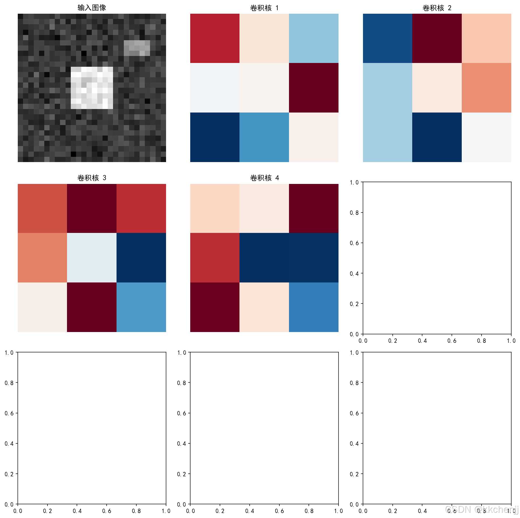
def demo5_photonic_cnn():
    """演示5: 光子卷积神经网络"""
    print("\n" + "=" * 60)
    print("演示5: 光子卷积神经网络")
    print("=" * 60)
    
    # 创建卷积层
    conv_layer = PhotonicConvLayer(kernel_size=3, n_kernels=4, stride=1)
    
    print(f"\n卷积层参数:")
    print(f"  卷积核大小: {conv_layer.kernel_size}x{conv_layer.kernel_size}")
    print(f"  卷积核数量: {conv_layer.n_kernels}")
    print(f"  步长: {conv_layer.stride}")
    
    # 生成测试图像 (简单模式)
    img_size = 28
    test_image = np.zeros((1, img_size, img_size, 1))
    
    # 添加一些特征
    test_image[0, 10:18, 10:18, 0] = 1.0  # 方块
    test_image[0, 5:8, 20:25, 0] = 0.5    # 小矩形
    
    # 添加噪声
    test_image += np.random.randn(1, img_size, img_size, 1) * 0.1
    
    # 前向传播
    output = conv_layer.forward(test_image)
    
    print(f"  输入形状: {test_image.shape}")
    print(f"  输出形状: {output.shape}")
    
    # 绘图
    fig, axes = plt.subplots(3, 3, figsize=(12, 12))
    
    # 1. 输入图像
    ax = axes[0, 0]
    ax.imshow(test_image[0, :, :, 0], cmap='gray')
    ax.set_title('输入图像')
    ax.axis('off')
    
    # 2. 卷积核
    for i in range(min(4, conv_layer.n_kernels)):
        row = (i + 1) // 3
        col = (i + 1) % 3
        ax = axes[row, col]
        ax.imshow(conv_layer.kernels[i], cmap='RdBu_r')
        ax.set_title(f'卷积核 {i+1}')
        ax.axis('off')
    
    # 3. 特征图
    fig2, axes2 = plt.subplots(2, 2, figsize=(10, 10))
    for i in range(min(4, conv_layer.n_kernels)):
        row = i // 2
        col = i % 2
        ax = axes2[row, col]
        ax.imshow(output[0, :, :, i], cmap='viridis')
        ax.set_title(f'特征图 {i+1}')
        ax.axis('off')
    
    plt.tight_layout()
    plt.savefig('cnn_feature_maps.png', dpi=150, bbox_inches='tight')
    print("\nCNN特征图已保存到 cnn_feature_maps.png")
    plt.close()
    
    # 保存卷积核图
    fig.tight_layout()
    plt.savefig('cnn_kernels.png', dpi=150, bbox_inches='tight')
    print("CNN卷积核图已保存到 cnn_kernels.png")
    plt.close()


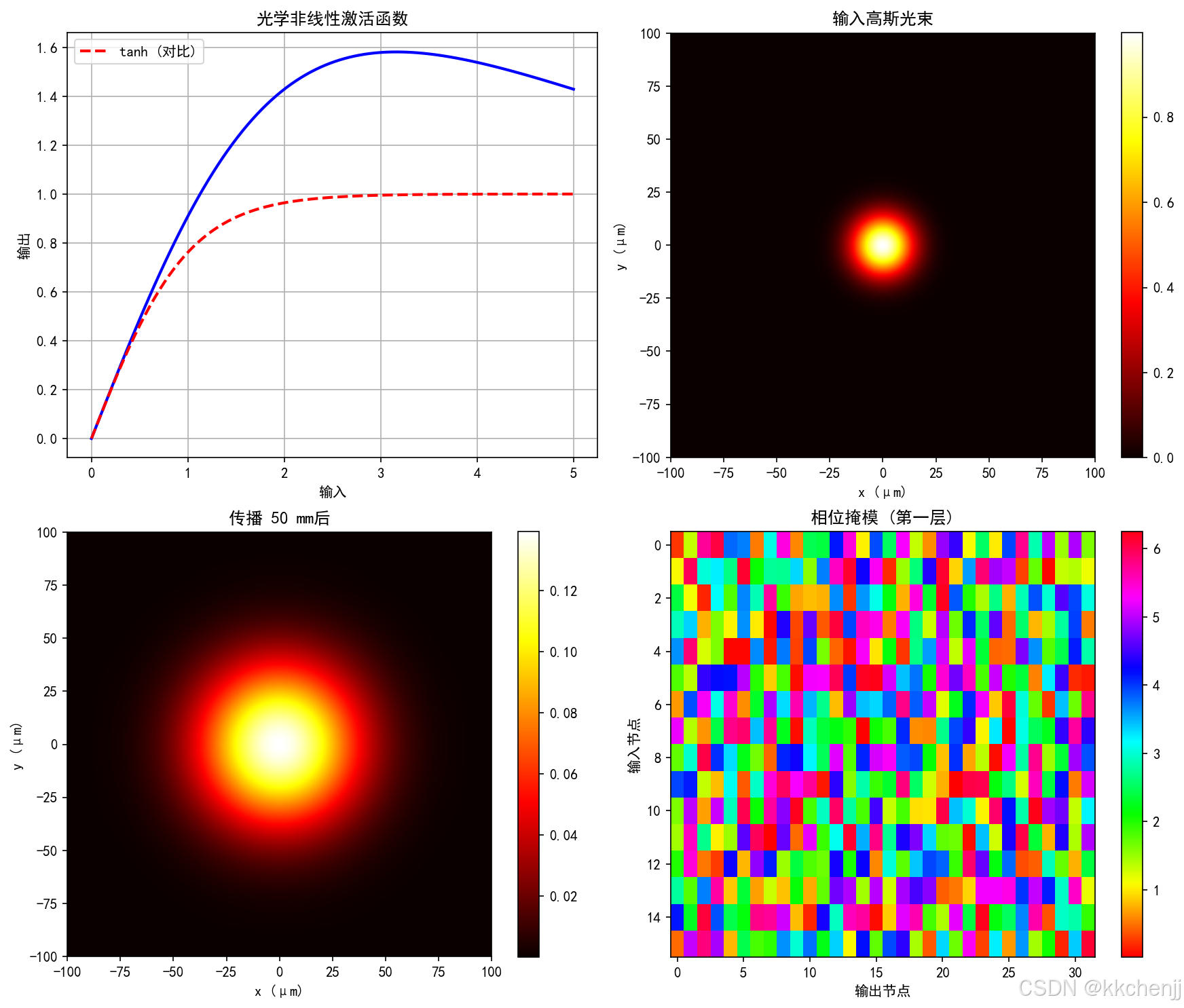
def demo6_all_optical_nn():
    """演示6: 全光神经网络"""
    print("\n" + "=" * 60)
    print("演示6: 全光神经网络")
    print("=" * 60)
    
    # 创建全光神经网络
    layer_sizes = [16, 32, 16, 4]
    optical_nn = AllOpticalNN(layer_sizes)
    
    print(f"\n网络架构: {layer_sizes}")
    print(f"  层数: {len(layer_sizes)}")
    print(f"  相位掩模数: {len(optical_nn.phase_masks)}")
    
    # 测试前向传播
    test_input = np.random.rand(layer_sizes[0])
    output = optical_nn.forward(test_input)
    
    print(f"  输入维度: {len(test_input)}")
    print(f"  输出维度: {len(output)}")
    
    # 光学非线性特性
    x_range = np.linspace(0, 5, 100)
    y_activation = optical_nn.optical_activation(x_range)
    
    # 角谱传播演示
    # 创建高斯光束
    x = np.linspace(-100e-6, 100e-6, 256)
    y = np.linspace(-100e-6, 100e-6, 256)
    X, Y = np.meshgrid(x, y)
    
    w0 = 20e-6  # 束腰
    E0 = np.exp(-(X**2 + Y**2) / w0**2)
    
    # 传播
    z_prop = 50e-3
    E_prop = optical_nn.angular_spectrum_propagation(E0, z_prop, x[1]-x[0])
    
    # 绘图
    fig, axes = plt.subplots(2, 2, figsize=(12, 10))
    
    # 1. 光学非线性激活函数
    ax1 = axes[0, 0]
    ax1.plot(x_range, y_activation, 'b-', linewidth=2)
    ax1.plot(x_range, np.tanh(x_range), 'r--', linewidth=2, label='tanh (对比)')
    ax1.set_xlabel('输入')
    ax1.set_ylabel('输出')
    ax1.set_title('光学非线性激活函数')
    ax1.legend()
    ax1.grid(True)
    
    # 2. 输入光场
    ax2 = axes[0, 1]
    im = ax2.imshow(np.abs(E0)**2, extent=[-100, 100, -100, 100], cmap='hot')
    ax2.set_xlabel('x (μm)')
    ax2.set_ylabel('y (μm)')
    ax2.set_title('输入高斯光束')
    plt.colorbar(im, ax=ax2)
    
    # 3. 传播后光场
    ax3 = axes[1, 0]
    im2 = ax3.imshow(np.abs(E_prop)**2, extent=[-100, 100, -100, 100], cmap='hot')
    ax3.set_xlabel('x (μm)')
    ax3.set_ylabel('y (μm)')
    ax3.set_title(f'传播 {z_prop*1e3:.0f} mm后')
    plt.colorbar(im2, ax=ax3)
    
    # 4. 相位掩模示例
    ax4 = axes[1, 1]
    im3 = ax4.imshow(optical_nn.phase_masks[0], cmap='hsv', aspect='auto')
    ax4.set_xlabel('输出节点')
    ax4.set_ylabel('输入节点')
    ax4.set_title('相位掩模 (第一层)')
    plt.colorbar(im3, ax=ax4)
    
    plt.tight_layout()
    plt.savefig('all_optical_nn.png', dpi=150, bbox_inches='tight')
    print("\n全光神经网络图已保存到 all_optical_nn.png")
    plt.close()


def demo7_neuromorphic_chip():
    """演示7: 光子神经形态芯片架构"""
    print("\n" + "=" * 60)
    print("演示7: 光子神经形态芯片架构")
    print("=" * 60)
    
    # 创建芯片
    chip = PhotonicNeuromorphicChip(n_cores=4, neurons_per_core=16)
    
    print(f"\n芯片架构参数:")
    print(f"  核心数: {chip.n_cores}")
    print(f"  每核心神经元: {chip.neurons_per_core}")
    print(f"  总神经元数: {chip.n_cores * chip.neurons_per_core}")
    print(f"  波分复用通道: {chip.n_wavelengths}")
    
    # 计算功耗
    power = chip.compute_power_consumption(activity_rate=0.1)
    print(f"\n功耗分析:")
    print(f"  激光器: {power['laser']*1e3:.2f} mW")
    print(f"  调制器: {power['modulator']*1e3:.2f} mW")
    print(f"  热调谐: {power['thermal']*1e3:.2f} mW")
    print(f"  总功耗: {power['total']*1e3:.2f} mW")
    
    # 计算吞吐量
    throughput = chip.compute_throughput(spike_rate=1e6)
    print(f"\n性能指标:")
    print(f"  吞吐量: {throughput:.2f} TOPS")
    print(f"  能效: {throughput / (power['total'] * 1e3):.2f} TOPS/W")
    
    # 仿真芯片运行
    dt = 0.1e-9
    t_max = 50e-9
    n_steps = int(t_max / dt)
    
    # 生成输入
    inputs = []
    for core_id in range(chip.n_cores):
        input_spikes = np.random.rand(chip.neurons_per_core, n_steps) < 0.05
        inputs.append(input_spikes)
    
    # 运行仿真
    outputs = chip.simulate_chip(inputs, dt, t_max)
    
    # 统计各核心发放率
    print(f"\n各核心发放统计:")
    for i, output in enumerate(outputs):
        firing_rate = np.sum(output) / (chip.neurons_per_core * t_max) / 1e9
        print(f"  核心 {i}: 发放率 = {firing_rate:.2f} GHz")
    
    # 绘图
    fig, axes = plt.subplots(2, 2, figsize=(12, 10))
    
    # 1. 芯片架构示意图
    ax1 = axes[0, 0]
    # 绘制核心布局
    core_positions = [(0.2, 0.2), (0.8, 0.2), (0.2, 0.8), (0.8, 0.8)]
    for i, (x, y) in enumerate(core_positions):
        circle = plt.Circle((x, y), 0.15, color=f'C{i}', alpha=0.7)
        ax1.add_patch(circle)
        ax1.text(x, y, f'Core\n{i}', ha='center', va='center', fontsize=10, color='white', weight='bold')
    
    # 绘制互连
    for i in range(len(core_positions)):
        for j in range(i+1, len(core_positions)):
            x1, y1 = core_positions[i]
            x2, y2 = core_positions[j]
            ax1.plot([x1, x2], [y1, y2], 'k-', alpha=0.3, linewidth=1)
    
    ax1.set_xlim(0, 1)
    ax1.set_ylim(0, 1)
    ax1.set_aspect('equal')
    ax1.axis('off')
    ax1.set_title('光子神经形态芯片架构')
    
    # 2. 功耗分布饼图
    ax2 = axes[0, 1]
    power_values = [power['laser']*1e3, power['modulator']*1e3, power['thermal']*1e3]
    power_labels = ['激光器', '调制器', '热调谐']
    colors = ['#ff9999', '#66b3ff', '#99ff99']
    ax2.pie(power_values, labels=power_labels, colors=colors, autopct='%1.1f%%', startangle=90)
    ax2.set_title('功耗分布')
    
    # 3. 核心间互连权重
    ax3 = axes[1, 0]
    im = ax3.imshow(chip.interconnect_weights, cmap='RdBu_r', aspect='auto', vmin=-0.2, vmax=0.2)
    ax3.set_xlabel('目标核心')
    ax3.set_ylabel('源核心')
    ax3.set_title('核心间互连权重')
    plt.colorbar(im, ax=ax3)
    
    # 4. 波分复用光谱
    ax4 = axes[1, 1]
    wavelengths_nm = chip.wavelengths * 1e9
    intensities = np.ones_like(wavelengths_nm)  # 理想情况
    ax4.bar(wavelengths_nm, intensities, width=2, color='steelblue', alpha=0.7)
    ax4.set_xlabel('波长 (nm)')
    ax4.set_ylabel('归一化强度')
    ax4.set_title('波分复用光谱')
    ax4.grid(True, alpha=0.3)
    
    plt.tight_layout()
    plt.savefig('neuromorphic_chip.png', dpi=150, bbox_inches='tight')
    print("\n神经形态芯片图已保存到 neuromorphic_chip.png")
    plt.close()


# ============================================================
# 主程序
# ============================================================

if __name__ == "__main__":
    # 运行所有演示
    demo1_photonic_neuron()
    demo2_optical_synapse()
    demo3_photonic_snn()
    demo4_reservoir_computing()
    demo5_photonic_cnn()
    demo6_all_optical_nn()
    demo7_neuromorphic_chip()
    
    print("\n" + "=" * 60)
    print("所有演示完成!")
    print("=" * 60)