基于卷积神经网络的生活垃圾识别系统,resnet50,alexnet, shufflenet模型【pytorch框架+python源码】
更多目标检测、图像分类识别、目标检测与追踪等项目可看我主页其他文章
功能演示 (看 shi pin 简介):
(一)简介
基于卷积神经网络的生活垃圾识别系统是在pytorch框架下实现的,这是一个完整的项目,包括代码,数据集,训练好的模型权重,模型训练记录,ui界面和各种模型指标图表等。
该项目有3个可选模型:resnet50,alexnet, shufflenet,3个模型都在项目中;GUI界面由tkinter设计和实现。此项目可在windowns、linux(ubuntu, centos)、mac系统下运行。
该项目是在pycharm和anaconda搭建的虚拟环境执行,pycharm和anaconda安装和配置可观看教程:
windows保姆级的pycharm+anaconda搭建python虚拟环境_windows启动python虚拟环境-CSDN博客
在Linux系统(Ubuntn, Centos)用pycharm+anaconda搭建python虚拟环境_linux pycharm-CSDN博客
(二)项目介绍
1. 项目结构
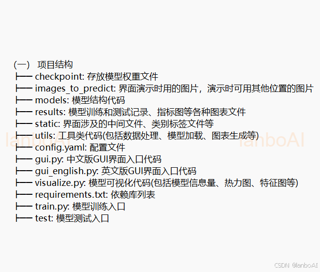
该项目可以使用已经训练好的模型权重,也可以自己重新训练,自己训练也比较简单
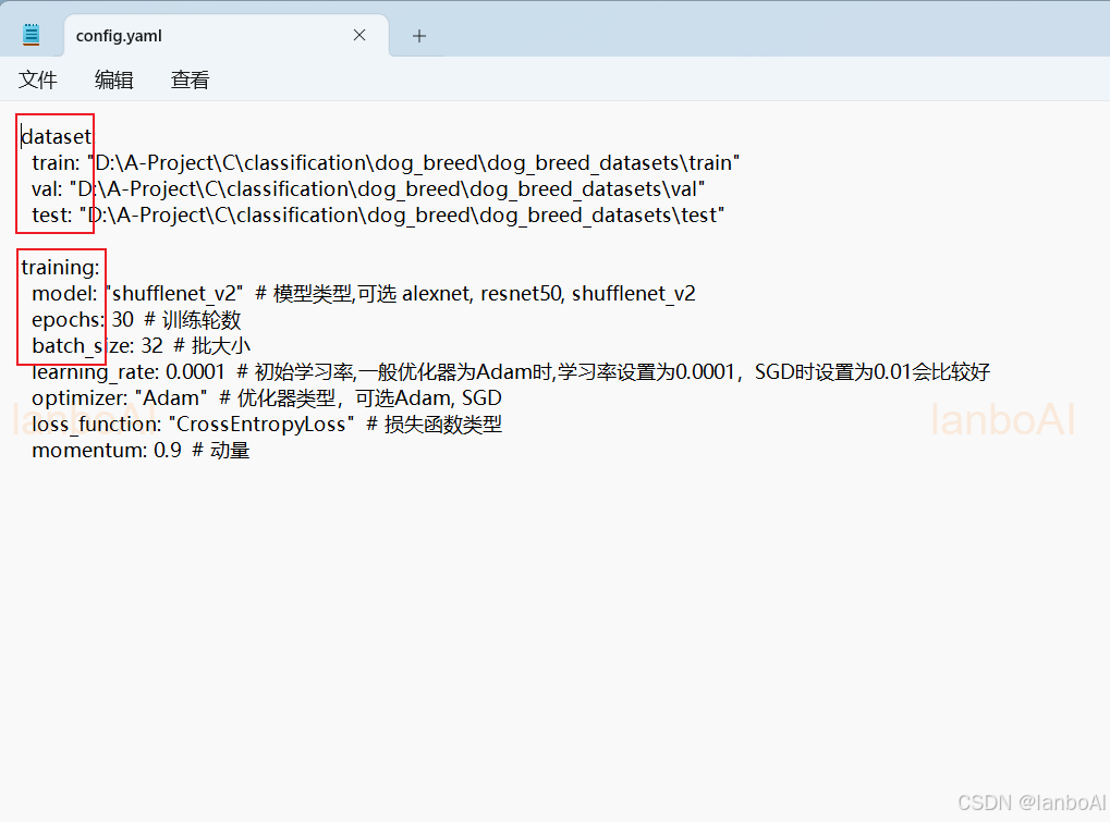
以训练shufflenet模型为例:
第一步:修改config.yaml文件中的数据集路径,模型名称、模型训练的轮数等
第二步:模型训练,即运行train.py文件
第三步:模型测试,即运行test.py文件
第四步:使用模型,即运行gui.py文件即可通过GUI界面来展示模型效果
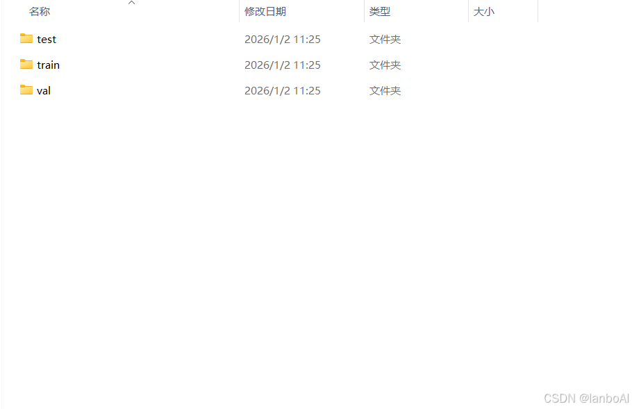
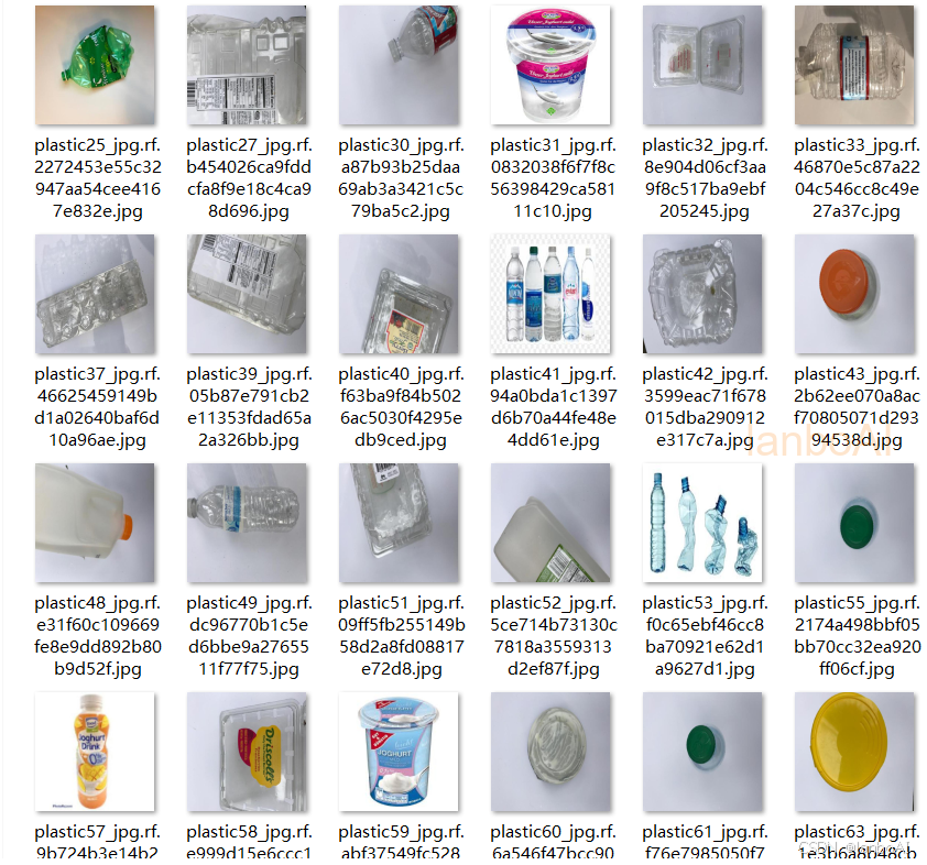
2. 数据结构
部分数据展示:
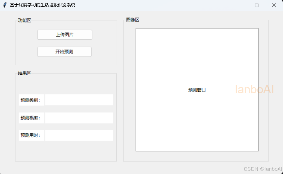
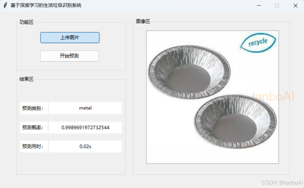
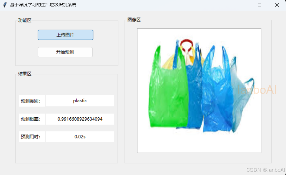
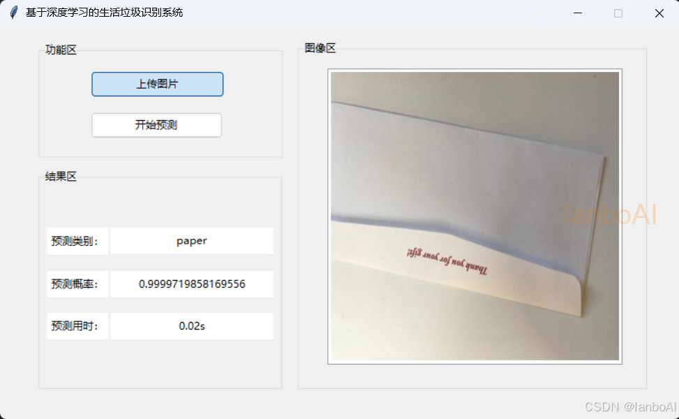
3.GUI界面(技术栈:tkinter+python)
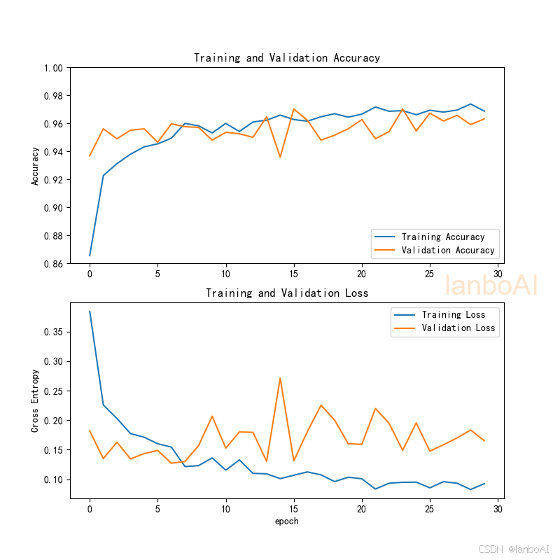
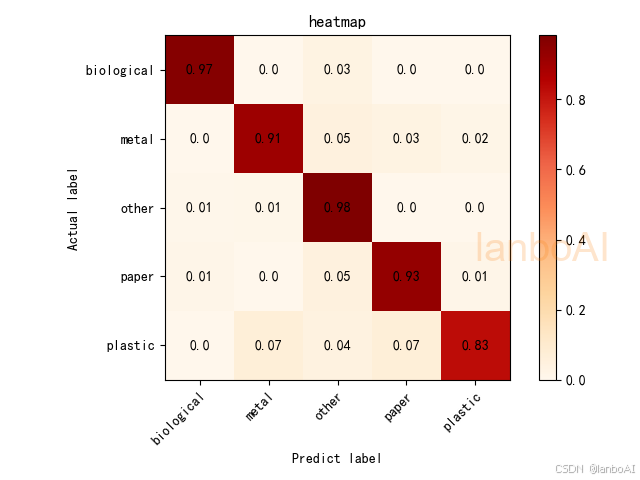
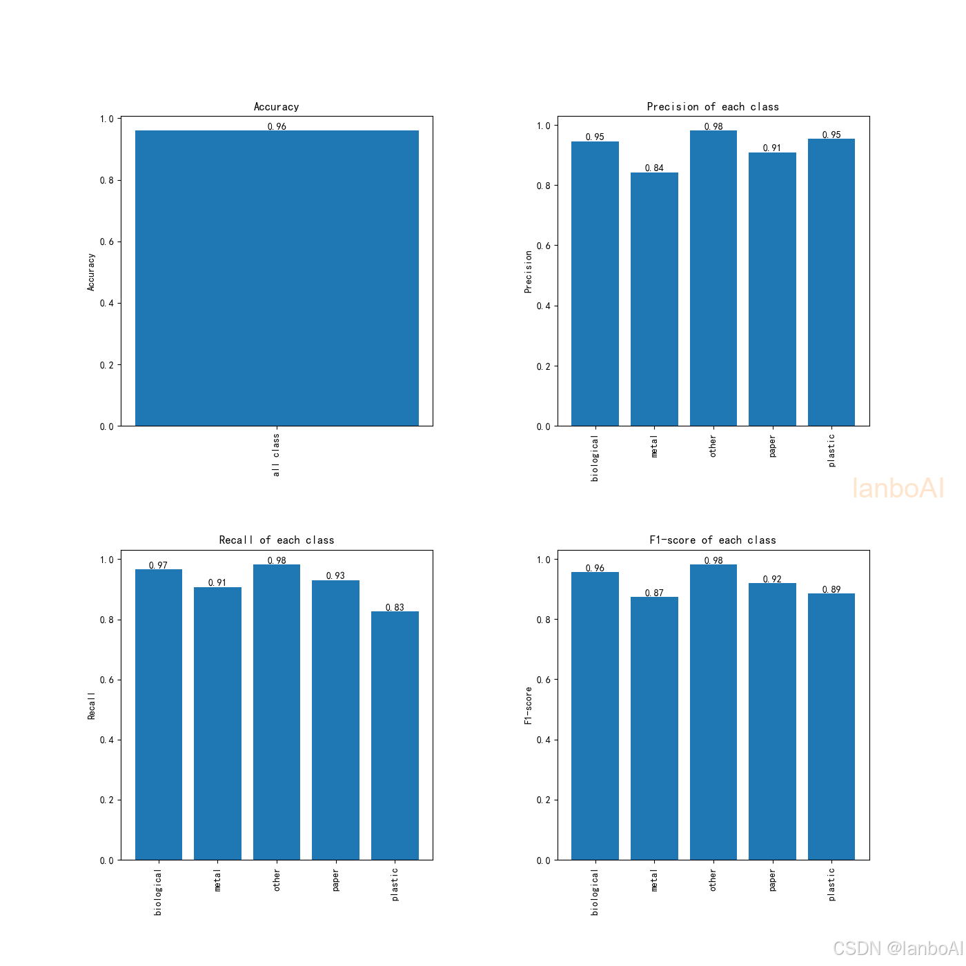
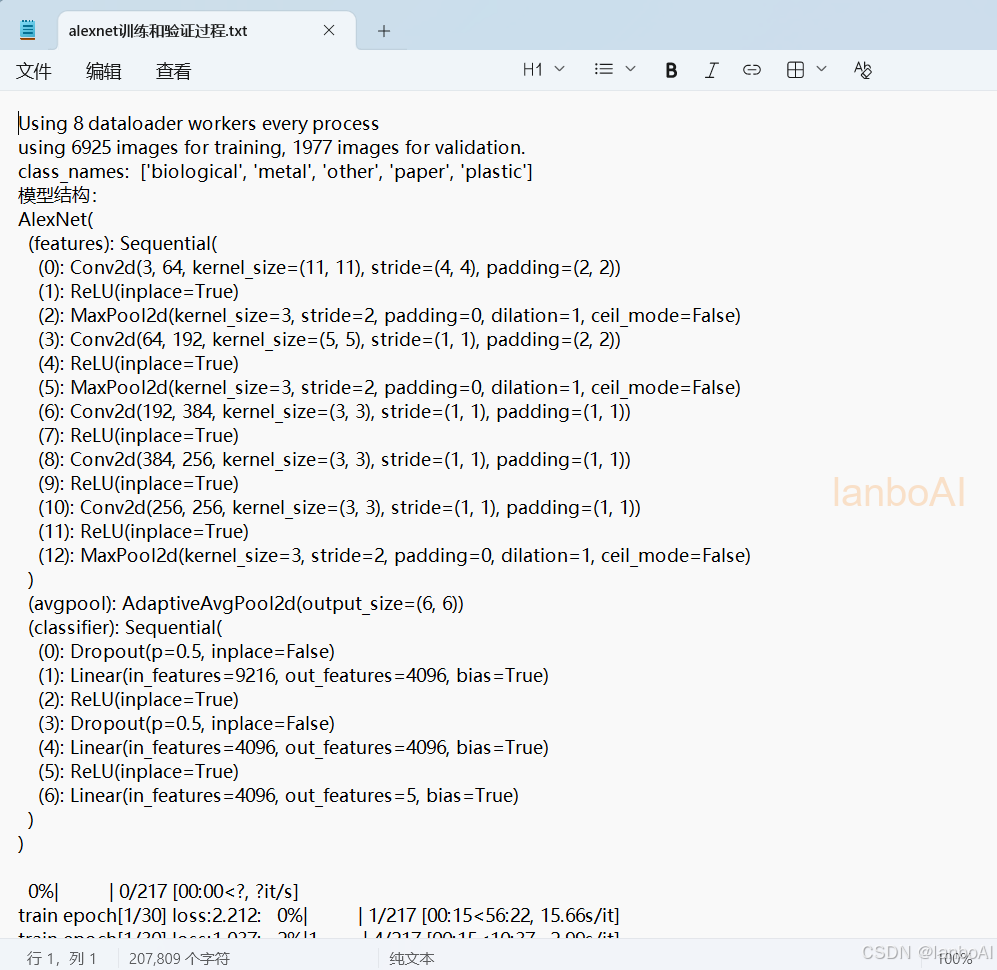
4.模型训练和验证的一些指标及效果
1)模型训练和验证的准确率曲线,损失曲线
2)分类混淆矩阵
3)准确率、精确率、召回率、F1值
4)模型训练和验证记录
(三)代码
由于篇幅有限,只展示核心代码
    def main(self, epochs):
        # 记录训练过程
        log_file_name = './results/resnet50训练和验证过程.txt'
        # 记录正常的 print 信息
        sys.stdout = Logger(log_file_name)

        # print("using {} device.".format(self.device))
        # 开始训练,记录开始时间
        begin_time = time()
        # 加载数据
        train_loader, validate_loader, class_names, train_num, val_num = self.data_load()
        print("class_names: ", class_names)
        train_steps = len(train_loader)  # 训练集批次数量
        val_steps = len(validate_loader)  # 验证集批次数量
        # 加载模型
        model = self.model_load()  # 创建模型

        # 网络结构可视化
        x = torch.randn(16, 3, 224, 224)  # 随机生成一个输入
        model_visual_path = 'results/resnet50_visual.onnx'  # 模型结构保存路径
        torch.onnx.export(model, x, model_visual_path)  # 将 pytorch 模型以 onnx 格式导出并保存
        # netron.start(model_visual_path)  # 浏览器会自动打开网络结构

        # load pretrain weights
        model_weight_path = "models/resnet50-pre.pth"  # 预训练模型权重路径
        assert os.path.exists(model_weight_path), "file {} does not exist.".format(model_weight_path)  # 权重文件是否存在
        model.load_state_dict(torch.load(model_weight_path, map_location='cpu'))  # 加载预训练模型权重

        # change fc layer structure
        in_channel = model.fc.in_features  # 获取fc层输入通道数
        model.fc = nn.Linear(in_channel, len(class_names))  # 修改fc层结构

        # 将模型放入GPU中或者CPU中
        model.to(self.device)
        # 定义损失函数,这里采用交叉熵损失函数
        loss_function = nn.CrossEntropyLoss()
        # 定义优化器
        params = [p for p in model.parameters() if p.requires_grad]  # 过滤不需要梯度更新的参数
        optimizer = optim.Adam(params=params, lr=0.0001)  # 优化器,这里采用Adam优化器,初始学习率为0.0001

        train_loss_history, train_acc_history = [], []  # 记录训练过程的损失和准确率
        test_loss_history, test_acc_history = [], []  # 记录验证过程的损失和准确率
        best_acc = 0.0  # 记录最佳准确率

        for epoch in range(0, epochs):  # 训练epochs次
            # 下面是模型训练
            model.train()  # 启用 BatchNormalization 和 Dropout
            running_loss = 0.0
            train_acc = 0.0
            train_bar = tqdm(train_loader, file=sys.stdout)  # 进度条
            # 进来一个batch的数据,计算一次梯度,更新一次网络
            for step, data in enumerate(train_bar):  # 遍历训练集数据
                images, labels = data  # 获取图像及对应的真实标签
                optimizer.zero_grad()  # 清空过往梯度
                outputs = model(images.to(self.device))  # 得到预测的标签
                train_loss = loss_function(outputs, labels.to(self.device))  # 计算损失
                train_loss.backward()  # 反向传播,计算当前梯度
                optimizer.step()  # 根据梯度更新网络参数

                # print statistics
                running_loss += train_loss.item()  # 累加损失
                predict_y = torch.max(outputs, dim=1)[1]  # 每行最大值的索引
                # torch.eq()进行逐元素的比较,若相同位置的两个元素相同,则返回True;若不同,返回False
                train_acc += torch.eq(predict_y, labels.to(self.device)).sum().item()  # 计算准确率
                train_bar.desc = "train epoch[{}/{}] loss:{:.3f}".format(epoch + 1,
                                                                         epochs,
                                                                         train_loss)  # 更新进度条
            # 下面是模型验证
            model.eval()  # 不启用 BatchNormalization 和 Dropout,保证BN和dropout不发生变化
            val_acc = 0.0  # accumulate accurate number / epoch
            testing_loss = 0.0
            with torch.no_grad():  # 张量的计算过程中无需计算梯度
                val_bar = tqdm(validate_loader, file=sys.stdout)  # 进度条
                for val_data in val_bar:  # 遍历验证集数据
                    val_images, val_labels = val_data  # 取出图像和标签
                    outputs = model(val_images.to(self.device))  # 模型推理

                    val_loss = loss_function(outputs, val_labels.to(self.device))  # 计算损失
                    testing_loss += val_loss.item()  # 累加损失

                    predict_y = torch.max(outputs, dim=1)[1]  # 每行最大值的索引
                    # torch.eq()进行逐元素的比较,若相同位置的两个元素相同,则返回True;若不同,返回False
                    val_acc += torch.eq(predict_y, val_labels.to(self.device)).sum().item()  # 计算准确率

            train_loss = running_loss / train_steps  # 计算平均损失
            train_accurate = train_acc / train_num  # 计算平均准确率
            test_loss = testing_loss / val_steps  # 计算平均损失
            val_accurate = val_acc / val_num  # 计算平均准确率

            train_loss_history.append(train_loss)
            train_acc_history.append(train_accurate)
            test_loss_history.append(test_loss)
            test_acc_history.append(val_accurate)

            print('[epoch %d] train_loss: %.3f  val_accuracy: %.3f' %
                  (epoch + 1, train_loss, val_accurate))
            if val_accurate > best_acc:
                best_acc = val_accurate
                torch.save(model.state_dict(), self.model_name)  # 保存最佳模型

        # 记录结束时间
        end_time = time()
        run_time = end_time - begin_time
        print('该循环程序运行时间:', run_time, "s")
        # 数据保存
        str_train_loss_history = ','.join([str(i) for i in train_loss_history])
        str_train_acc_history = ','.join([str(i) for i in train_acc_history])
        str_test_loss_history = ','.join([str(i) for i in test_loss_history])
        str_test_acc_history = ','.join([str(i) for i in test_acc_history])
        with open('results/resnet50_loss_acc.txt', 'w') as f:
            f.write("train_loss_history: " + str_train_loss_history + "\n")
            f.write("train_acc_history: " + str_train_acc_history + "\n")
            f.write("test_loss_history: " + str_test_loss_history + "\n")
            f.write("test_acc_history: " + str_test_acc_history + "\n")
        # 绘制模型训练过程图
        self.show_loss_acc(train_loss_history, train_acc_history,
                           test_loss_history, test_acc_history)
        # 画热力图
        test_real_labels, test_pre_labels = self.heatmaps(model, validate_loader, class_names)
        # 计算混淆矩阵
self.calculate_confusion_matrix(test_real_labels, test_pre_labels, class_names)(四)总结
以上即为整个项目的介绍,整个项目主要包括以下内容:完整的程序代码文件、训练好的模型、数据集、UI界面和各种模型指标图表等。
项目包含全部资料,一步到位,省心省力!
项目运行过程如出现问题,请及时交流!

AtomGit 是由开放原子开源基金会联合 CSDN 等生态伙伴共同推出的新一代开源与人工智能协作平台。平台坚持“开放、中立、公益”的理念,把代码托管、模型共享、数据集托管、智能体开发体验和算力服务整合在一起,为开发者提供从开发、训练到部署的一站式体验。
更多推荐

 3
3 0
0- 0


 已为社区贡献10条内容

所有评论(0)