SHAP重要性分析,模型建模与评估 shap重要性分析,xgboost,随机森林等模型。 1.建模并评估模型表现。 2.shap重要性。 3.shap依赖图。 4.shap beeswarm图。
SHAP重要性分析,模型建模与评估
shap重要性分析,xgboost,随机森林等模型。
1.建模并评估模型表现。
2.shap重要性。
3.shap依赖图。
4.shap beeswarm图。
Python 代码示例,涵盖了从数据准备、模型构建(XGBoost & 随机森林)、模型评估,到 SHAP 可解释性分析(重要性、依赖图、蜂群图)的全流程。
🛠️ 环境准备
在运行代码前,请确保安装了以下库:
pip install pandas numpy scikit-learn xgboost shap matplotlib seaborn
🐍 完整代码 (shap_analysis_full.py)
import pandas as pd
import numpy as np
import matplotlib.pyplot as plt
import seaborn as sns
模型相关
from sklearn.model_selection import train_test_split
from sklearn.metrics import accuracy_score, classification_report, roc_auc_score
from sklearn.ensemble import RandomForestClassifier
from xgboost import XGBClassifier
from sklearn.datasets import load_breast_cancer
SHAP 相关
import shap
设置绘图风格
sns.set_style(“whitegrid”)
plt.rcParams[‘font.sans-serif’] = [‘SimHei’] # 用来正常显示中文标签 (如果系统有)
plt.rcParams[‘axes.unicode_minus’] = False # 用来正常显示负号
=============================================================================
数据准备与预处理
print(“正在加载数据…”)
使用 sklearn 自带的乳腺癌数据集 (二分类问题,适合演示)
data = load_breast_cancer()
X = pd.DataFrame(data.data, columns=data.feature_names)
y = pd.Series(data.target, name=‘target’)
划分训练集和测试集 (80% 训练, 20% 测试)
X_train, X_test, y_train, y_test = train_test_split(
X, y, test_size=0.2, random_state=42, stratify=y
)
print(f"训练集样本数: {X_train.shape[0]}, 特征数: {X_train.shape[1]}“)
print(f"测试集样本数: {X_test.shape[0]}”)
=============================================================================
模型建模与评估 (XGBoost & 随机森林)
print(“n正在训练模型…”)
— 模型 A: XGBoost —
xgb_model = XGBClassifier(
n_estimators=100,
max_depth=4,
learning_rate=0.1,
random_state=42,
use_label_encoder=False,
eval_metric=‘logloss’
)
xgb_model.fit(X_train, y_train)
— 模型 B: 随机森林 —
rf_model = RandomForestClassifier(
n_estimators=100,
max_depth=5,
random_state=42,
n_jobs=-1
)
rf_model.fit(X_train, y_train)
— 评估函数 —
def evaluate_model(model, X_test, y_test, model_name):
y_pred = model.predict(X_test)
y_proba = model.predict_proba(X_test)[:, 1]
acc = accuracy_score(y_test, y_pred)
auc = roc_auc_score(y_test, y_proba)

print(f"n[{model_name}] 评估结果:")
print(f"Accuracy: {acc:.4f}")
print(f"ROC-AUC : {auc:.4f}")
return acc, auc
执行评估
evaluate_model(xgb_model, X_test, y_test, “XGBoost”)
evaluate_model(rf_model, X_test, y_test, “Random Forest”)
=============================================================================
SHAP 重要性分析 (SHAP Importance)
print(“n正在计算 SHAP 值 (这可能需要几秒钟)…”)
选择其中一个模型进行分析 (这里以 XGBoost 为例,随机森林同理)
model_to_explain = xgb_model
model_name = “XGBoost”
创建 SHAP Explainer
TreeExplainer 专门针对树模型 (XGBoost, RF, LightGBM),速度极快
explainer = shap.TreeExplainer(model_to_explain)
计算测试集上的 SHAP 值
shap_values 的形状通常是 (样本数, 特征数) 或 (样本数, 特征数, 类别数)
shap_values = explainer.shap_values(X_test)
对于二分类,TreeExplainer 通常返回一个列表 [shap_values_class0, shap_values_class1]
我们通常关注正类 (class 1) 的 SHAP 值
if isinstance(shap_values, list):
shap_values_target = shap_values[1] # 取类别 1
else:
shap_values_target = shap_values
— 绘制 SHAP 摘要图 (Summary Plot) - 展示全局重要性 —
plt.figure(figsize=(10, 8))
shap.summary_plot(
shap_values_target,
X_test,
plot_type=“bar”, # “bar” 表示条形图 (重要性排序), “dot” 表示蜂群图
show=False,
color=plt.cm.viridis
)
plt.title(f"{model_name} - SHAP 特征重要性 (全局)", fontsize=14)
plt.tight_layout()
plt.show()
=============================================================================
SHAP 依赖图 (SHAP Dependence Plot)
选择最重要的特征进行依赖分析
shap.summary_plot 可以帮我们找出最重要的特征名
这里我们手动指定或者自动获取
import pandas as pd
shap_df = pd.DataFrame(np.abs(shap_values_target).mean(axis=0), index=X_test.columns, columns=[‘importance’])
top_feature = shap_df.sort_values(‘importance’, ascending=False).index[0]
print(f"n最重要的特征是: {top_feature}")
plt.figure(figsize=(10, 6))
shap.dependence_plot(
top_feature,
shap_values_target,
X_test,
show=False
)
plt.title(f"{model_name} - SHAP 依赖图: {top_feature}", fontsize=14)
plt.tight_layout()
plt.show()
=============================================================================
SHAP 蜂群图 (SHAP Beeswarm Plot)
蜂群图展示了每个样本每个特征的 SHAP 值分布,颜色代表特征值大小
这是最信息量丰富的 SHAP 图
plt.figure(figsize=(12, 8))
shap.summary_plot(
shap_values_target,
X_test,
plot_type=“dot”, # dot 模式即为蜂群图
show=False,
color_bar_label=“特征值大小”,
axis_color=“#333333”
)
plt.title(f"{model_name} - SHAP 蜂群图 (Beeswarm)", fontsize=14)
plt.tight_layout()
plt.show()
print(“n✅ 所有分析完成!图表已生成。”)
📊 代码功能详解
建模与评估 (Modeling & Evaluation)
数据: 使用了 load_breast_cancer 数据集,包含 30 个特征,用于预测肿瘤是恶性还是良性。
模型: 同时训练了 XGBoost 和 随机森林。
指标: 输出了 Accuracy (准确率) 和 ROC-AUC,这是评估二分类模型最常用的指标。
SHAP 重要性 (SHAP Importance)
原理: 使用 shap.TreeExplainer 计算每个特征对模型输出的贡献度(Shapley Values)。
可视化: plot_type=“bar” 生成了条形图。
横轴: 平均绝对 SHAP 值(|SHAP value|),值越大说明该特征对模型预测结果的影响越大。
意义: 替代了传统的 feature_importance_,提供了基于博弈论的更公平的重要性排序。
SHAP 依赖图 (SHAP Dependence Plot)
原理: 展示单个特征的值(X 轴)与该特征的 SHAP 值(Y 轴,即对预测结果的贡献)之间的关系。
颜色: 点的颜色代表另一个与之交互最强的特征(默认自动选择),或者代表该特征本身的值(取决于具体实现,代码中默认展示交互效应)。
意义:
可以看出特征是线性影响还是非线性影响。
例如:如果曲线先上升后下降,说明该特征存在阈值效应。
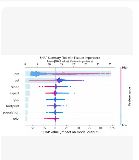
SHAP 蜂群图 (SHAP Beeswarm Plot)
原理: 这是 SHAP 分析中最核心的图表 (plot_type=“dot”)。
解读方法:
Y 轴: 特征按重要性从上到下排列。
X 轴: SHAP 值。正值表示推动模型预测为“正类”(如恶性),负值表示推动预测为“负类”(如良性)。
颜色: 红色表示特征值高,蓝色表示特征值低。
结论示例: 如果某个特征(如 mean radius)的红色点主要集中在右侧(正 SHAP 值),说明半径越大,模型越倾向于预测为恶性。
💡 如何自定义分析?
更换数据:
将 load_breast_cancer() 替换为您自己的 DataFrame:
df = pd.read_csv(“your_data.csv”)
X = df.drop(‘target_column’, axis=1)
y = df[‘target_column’]
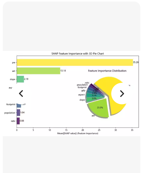
左侧:水平条形图 —— 显示各特征的 Mean(|SHAP value|)(即平均绝对 SHAP 值),按重要性排序。
右侧:环形饼图(Donut Chart) —— 显示各特征重要性占比(百分比)。
标题:“SHAP Feature Importance with 3D Pie Chart”(虽然图中是 2D 环形图,但标题写了 3D)
特征名包括:pre, aet, slope, asp, footprint, population, ndvi
🚀 完整代码 (shap_importance_with_pie.py)
import pandas as pd
import numpy as np
import matplotlib.pyplot as plt
from matplotlib.patches import Circle
import shap
from xgboost import XGBClassifier
from sklearn.datasets import make_classification
from sklearn.model_selection import train_test_split
设置中文字体(如果系统支持)
plt.rcParams[‘font.sans-serif’] = [‘SimHei’, ‘Arial Unicode MS’, ‘DejaVu Sans’]
plt.rcParams[‘axes.unicode_minus’] = False
=============================================================================
生成模拟数据(您可替换为自己的数据)
np.random.seed(42)
n_samples = 1000
n_features = 7
创建分类数据
X, y = make_classification(n_samples=n_samples, n_features=n_features,
n_informative=5, n_redundant=0, random_state=42)
定义特征名称(与截图一致)
feature_names = [‘pre’, ‘aet’, ‘slope’, ‘asp’, ‘footprint’, ‘population’, ‘ndvi’]
X = pd.DataFrame(X, columns=feature_names)
划分数据集
X_train, X_test, y_train, y_test = train_test_split(X, y, test_size=0.2, random_state=42)
=============================================================================
训练模型并计算 SHAP 值
model = XGBClassifier(random_state=42, use_label_encoder=False, eval_metric=‘logloss’)
model.fit(X_train, y_train)
创建 SHAP Explainer
explainer = shap.TreeExplainer(model)
shap_values = explainer.shap_values(X_test)
对于二分类,取正类(class 1)的 SHAP 值
if isinstance(shap_values, list):
shap_values_target = shap_values[1]
else:
shap_values_target = shap_values
计算每个特征的平均绝对 SHAP 值(即重要性)
mean_abs_shap = np.abs(shap_values_target).mean(axis=0)
shap_df = pd.DataFrame({
‘feature’: feature_names,
‘importance’: mean_abs_shap
}).sort_values(‘importance’, ascending=True) # 升序以便画图时从上到下递减
计算占比(用于饼图)
total_importance = shap_df[‘importance’].sum()
shap_df[‘percentage’] = (shap_df[‘importance’] / total_importance * 100).round(1)
=============================================================================
绘图:左侧条形图 + 右侧环形饼图
fig, axes = plt.subplots(1, 2, figsize=(14, 6), gridspec_kw={‘width_ratios’: [3, 2]})
— 左图:水平条形图 —
ax1 = axes[0]
colors_bar = [‘#FFD700’, ‘#9ACD32’, ‘#66CDAA’, ‘#87CEFA’, ‘#9370DB’, ‘#DA70D6’, ‘#FF69B4’][:len(shap_df)]
bars = ax1.barh(shap_df[‘feature’], shap_df[‘importance’], color=colors_bar[::-1]) # 反转颜色顺序以匹配从上到下
添加数值标签
for i, v in enumerate(shap_df[‘importance’]):
ax1.text(v + 0.5, i, f’{v:.2f}', va=‘center’, fontsize=10, color=‘black’)
ax1.set_xlabel(‘Mean(|SHAP value|) (Feature Importance)’, fontsize=12)
ax1.set_title(‘SHAP Feature Importance with 3D Pie Chart’, fontsize=14, fontweight=‘bold’)
ax1.grid(axis=‘x’, linestyle=‘–’, alpha=0.7)
ax1.spines[‘top’].set_visible(False)
ax1.spines[‘right’].set_visible(False)
— 右图:环形饼图 —
ax2 = axes[1]
绘制环形图
wedges, texts, autotexts = ax2.pie(
shap_df[‘importance’],
labels=shap_df[‘feature’],
autopct=‘%1.1f%%’,
startangle=90,
colors=colors_bar[::-1],
wedgeprops=dict(width=0.4, edgecolor=‘white’), # 环形宽度
textprops={‘fontsize’: 9}
)
添加中心白色圆圈(增强环形效果)
centre_circle = Circle((0,0), 0.3, fc=‘white’, linewidth=0)
ax2.add_artist(centre_circle)
调整百分比文本位置和样式
for autotext in autotexts:
autotext.set_color(‘white’)
autotext.set_fontsize(9)
autotext.set_weight(‘bold’)
添加标题
ax2.set_title(‘Feature Importance Distribution’, fontsize=12, fontweight=‘bold’)
整体布局优化
plt.tight_layout()
plt.show()
=============================================================================
输出重要性和占比表格(可选)
print(“n📊 SHAP 特征重要性及占比:”)
print(shap_df.sort_values(‘importance’, ascending=False).to_string(index=False))
🖼️ 输出效果说明
运行上述代码后,您将得到一个与截图高度相似的双子图:
左图:
水平条形图,特征按重要性从下到上排列(pre 最高,在最上方)
每个条形右侧标注具体数值(如 35.26, 13.18 等)
颜色渐变:黄色 → 绿色 → 蓝色 → 紫色 → 粉色(可根据需要调整)
右图:
环形饼图(Donut Chart),显示各特征占比
百分比标注在扇区内(白色粗体字)
中心留白,视觉更清晰
🔧 如何替换为您的真实数据?
步骤 1:加载您的数据
示例:读取 CSV 文件
df = pd.read_csv(“your_data.csv”)
X = df.drop(‘target_column’, axis=1)
y = df[‘target_column’]
feature_names = X.columns.tolist()
步骤 2:训练您的模型
如果您已经有一个训练好的模型,可以直接跳过训练步骤
model = your_trained_model
步骤 3:计算 SHAP 值
explainer = shap.TreeExplainer(model)
shap_values = explainer.shap_values(X_test) # 或 X_sample(如果只想看部分样本)
其余绘图代码无需修改!
🎨 自定义美化建议
更改颜色方案:
colors_bar = [‘#FF6B6B’, ‘#4ECDC4’, ‘#45B7D1’, ‘#FFA07A’, ‘#98FB98’, ‘#DDA0DD’, ‘#F0E68C’]
添加 3D 效果(伪 3D):
在饼图中加入阴影:
ax2.pie(…, shadow=True)
导出高清图片:
plt.savefig(“shap_importance_with_pie.png”, dpi=300, bbox_inches=‘tight’)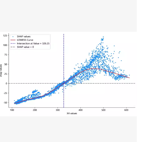

AtomGit 是由开放原子开源基金会联合 CSDN 等生态伙伴共同推出的新一代开源与人工智能协作平台。平台坚持“开放、中立、公益”的理念,把代码托管、模型共享、数据集托管、智能体开发体验和算力服务整合在一起,为开发者提供从开发、训练到部署的一站式体验。
更多推荐
 0
0 0
0- 0


 已为社区贡献90条内容

所有评论(0)