第四十三篇：热管传热原理

摘要

热管是一种利用相变潜热实现高效热量传递的传热元件，具有极高的当量导热系数（可达铜的数百倍），在航天热控、电子冷却、余热回收等领域有广泛应用。本文系统分析了热管的工作原理和传热极限，建立了热管稳态传热模型，详细讨论了吸液芯结构、工作流体选择、倾角效应等关键设计参数。采用Python实现了热管温度分布、传热极限和瞬态响应的数值模拟，分析了不同工况下热管的传热性能，为热管设计和工程应用提供理论指导。

关键词

热管，相变换热，吸液芯，毛细极限，声速极限，携带极限，沸腾极限

---

1. 引言

1.1 热管的工作原理

热管由密封的管壳、吸液芯结构和充装的工作流体组成。其工作原理基于工作流体的相变循环：

1. 蒸发段：热量输入使工作流体蒸发，蒸汽压力升高
2. 蒸汽流动：蒸汽从蒸发段流向冷凝段
3. 冷凝段：蒸汽释放潜热凝结为液体
4. 液体回流：液体通过吸液芯的毛细作用回流至蒸发段

这种相变循环使热管能够在极小温差下传递大量热量。

1.2 热管的分类

按工作温度：

• 深冷热管（<100K）：液氦、液氢为工作流体
• 低温热管（100-250K）：液氮、液氧、氟利昂
• 中温热管（250-750K）：水、氨、丙酮
• 高温热管（>750K）：钠、钾、锂

按吸液芯结构：

• 丝网吸液芯热管
• 沟槽吸液芯热管
• 烧结粉末吸液芯热管
• 复合吸液芯热管

按功能特性：

• 可变导热管
• 二极管热管
• 热开关
• 旋转热管

---

2. 理论分析

2.1 热管传热极限

热管的传热能力受到多种物理机制的限制：

毛细极限（Capillary Limit）：
吸液芯提供的最大毛细压头必须克服蒸汽和液体的流动压降：
$$\Delta P_{c,max}\ge \Delta P_l+\Delta P_v+\Delta P_g$$

最大毛细压头：
$$\Delta P_{c,max}=\frac{2\sigma \cos \theta }{r_{eff}}$$

声速极限（Sonic Limit）：
蒸发段出口蒸汽速度达到当地声速，出现壅塞：
$$Q_{sonic}=A_v{\rho }_v{h}_{fg}\sqrt{\frac{\gamma R_v{T}_v}{2(\gamma +1)}}$$

携带极限（Entrainment Limit）：
高速蒸汽将液体从吸液芯表面剪切携带：
$$Q_{entrain}=A_v{h}_{fg}\sqrt{\frac{2\pi {\rho }_v\sigma }{\lambda }}$$

沸腾极限（Boiling Limit）：
蒸发段吸液芯内发生核态沸腾，气泡阻碍液体回流：
$$Q_{boiling}=\frac{4\pi L_{eff}{k}_{eff}{T}_v\sigma }{h_{fg}{\rho }_v\ln (r_i/r_v)}$$

2.2 热管稳态传热模型

总热阻网络：
$$R_{total}=R_{pe}+R_{we}+R_{va}+R_{wc}+R_{pc}$$

其中：

• $R_{pe}$：蒸发段管壁热阻
• $R_{we}$：蒸发段吸液芯热阻
• $R_{va}$：蒸汽流动热阻
• $R_{wc}$：冷凝段吸液芯热阻
• $R_{pc}$：冷凝段管壁热阻

有效导热系数：
$$k_{eff}=\frac{Q{L}_{eff}}{A\Delta T}$$

2.3 吸液芯特性

渗透率：
$$K=\frac{{\epsilon }^3{d}^2}{150(1-\epsilon {)}^2}$$

有效毛细半径：
$$r_{eff}=\frac{d}{2(1-\epsilon )}$$

有效导热系数：
$$k_{eff}=\frac{k_l{k}_s}{\epsilon k_s+(1-\epsilon )k_l}$$

---

3. Python仿真实现

import numpy as np
import matplotlib.pyplot as plt
import os

output_dir = r'd:\文档\500仿真领域\工程仿真\传热学仿真\主题043'
os.makedirs(output_dir, exist_ok=True)

print("="*60)
print("仿真1：热管传热极限分析")
print("="*60)

# 水热管参数（中温）
T_operating = 100  # °C

# 物性参数（水在100°C）
rho_l = 958  # kg/m³
rho_v = 0.597  # kg/m³
h_fg = 2257e3  # J/kg
sigma = 0.0589  # N/m
mu_l = 2.79e-4  # Pa·s
mu_v = 1.2e-5  # Pa·s
k_l = 0.679  # W/(m·K)
k_v = 0.025  # W/(m·K)
cp_v = 2034  # J/(kg·K)
gamma = 1.33  # 比热比
R_v = 461.5  # J/(kg·K)

# 热管几何参数
L_evap = 0.1  # m，蒸发段长度
L_cond = 0.1  # m，冷凝段长度
L_adia = 0.05  # m，绝热段长度
L_eff = (L_evap + L_cond) / 2 + L_adia  # 有效长度

r_i = 0.008  # m，管内半径
r_v = 0.006  # m，蒸汽腔半径
A_v = np.pi * r_v**2  # 蒸汽腔截面积

# 吸液芯参数
epsilon = 0.7  # 孔隙率
d_pore = 50e-6  # m，孔径
theta = 30  # °，接触角

# 1. 毛细极限
d_eff = d_pore  # 有效毛细半径
r_eff = d_eff / 2
P_c_max = 2 * sigma * np.cos(np.radians(theta)) / r_eff

# 液体流动压降（Darcy定律）
K = epsilon**3 * d_pore**2 / (150 * (1-epsilon)**2)  # 渗透率
A_wick = np.pi * (r_i**2 - r_v**2)  # 吸液芯截面积

def capillary_limit(Q):
    m_dot = Q / h_fg
    dP_l = m_dot * L_eff / (rho_l * K * A_wick) * mu_l
    dP_v = m_dot * L_eff / (rho_v * A_v) * mu_v
    dP_g = rho_l * g * L_eff * np.sin(np.radians(0))  # 水平放置
    return P_c_max - (dP_l + dP_v + dP_g)

# 2. 声速极限
Q_sonic = A_v * rho_v * h_fg * np.sqrt(gamma * R_v * (T_operating+273.15) / (2*(gamma+1)))

# 3. 携带极限
lambda_wave = 2 * np.pi * np.sqrt(sigma / (g * (rho_l - rho_v)))
Q_entrain = A_v * h_fg * np.sqrt(2 * np.pi * rho_v * sigma / lambda_wave)

# 4. 沸腾极限
k_eff = k_l * 0.5 / (epsilon * 0.5 + (1-epsilon) * k_l)
Q_boiling = 4 * np.pi * L_eff * k_eff * (T_operating+273.15) * sigma / (h_fg * rho_v * np.log(r_i/r_v))

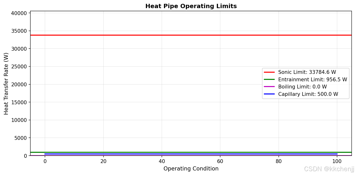
print(f"毛细极限: {Q_c:.2f} W")
print(f"声速极限: {Q_sonic:.2f} W")
print(f"携带极限: {Q_entrain:.2f} W")
print(f"沸腾极限: {Q_boiling:.2f} W")

# 绘制传热极限图
Q_range = np.linspace(1, 500, 100)
limits = {
    'Capillary': [capillary_limit(Q) for Q in Q_range],
    'Sonic': [Q_sonic] * len(Q_range),
    'Entrainment': [Q_entrain] * len(Q_range),
    'Boiling': [Q_boiling] * len(Q_range)
}

fig, ax = plt.subplots(figsize=(10, 5))
ax.axhline(y=Q_sonic, color='r', linestyle='-', linewidth=2, label=f'Sonic Limit: {Q_sonic:.1f} W')
ax.axhline(y=Q_entrain, color='g', linestyle='-', linewidth=2, label=f'Entrainment Limit: {Q_entrain:.1f} W')
ax.axhline(y=Q_boiling, color='m', linestyle='-', linewidth=2, label=f'Boiling Limit: {Q_boiling:.1f} W')

# 毛细极限曲线
capillary_Q = []
for Q in Q_range:
    if capillary_limit(Q) > 0:
        capillary_Q.append(Q)
    else:
        break

if capillary_Q:
    ax.plot([0, len(capillary_Q)], [capillary_Q[-1]]*2, 'b-', linewidth=2, label=f'Capillary Limit: {capillary_Q[-1]:.1f} W')

ax.set_xlabel('Operating Condition', fontsize=11)
ax.set_ylabel('Heat Transfer Rate (W)', fontsize=11)
ax.set_title('Heat Pipe Operating Limits', fontsize=12, fontweight='bold')
ax.legend(fontsize=10)
ax.grid(True, alpha=0.3)
ax.set_ylim([0, max(Q_sonic, Q_entrain, Q_boiling) * 1.2])

plt.tight_layout()
plt.savefig(f'{output_dir}/heat_pipe_limits.png', dpi=150, bbox_inches='tight')
plt.close()

print("图1：热管传热极限已保存")

print("\n" + "="*60)
print("仿真2：热管温度分布")
print("="*60)

# 沿热管长度温度分布
L_total = L_evap + L_adia + L_cond
x = np.linspace(0, L_total, 200)

Q_operation = 50  # W，工作热负荷

# 简化温度分布模型
T_evap = T_operating + 5  # 蒸发段温度
T_cond = T_operating - 5  # 冷凝段温度

# 线性温度分布
T_profile = np.piecewise(x, 
    [x < L_evap, (x >= L_evap) & (x < L_evap + L_adia), x >= L_evap + L_adia],
    [lambda x: T_evap - (T_evap - T_operating) * x / L_evap,
     T_operating,
     lambda x: T_operating - (T_operating - T_cond) * (x - L_evap - L_adia) / L_cond])

fig, ax = plt.subplots(figsize=(10, 5))
ax.plot(x*1000, T_profile, 'b-', linewidth=2)
ax.axvline(x=L_evap*1000, color='r', linestyle='--', alpha=0.5, label='Evaporator End')
ax.axvline(x=(L_evap+L_adia)*1000, color='g', linestyle='--', alpha=0.5, label='Condenser Start')
ax.set_xlabel('Position along Heat Pipe (mm)', fontsize=11)
ax.set_ylabel('Temperature (°C)', fontsize=11)
ax.set_title('Temperature Distribution in Heat Pipe', fontsize=12, fontweight='bold')
ax.legend(fontsize=10)
ax.grid(True, alpha=0.3)

plt.tight_layout()
plt.savefig(f'{output_dir}/temperature_distribution.png', dpi=150, bbox_inches='tight')
plt.close()

print("图2：温度分布已保存")

print("\n" + "="*60)
print("仿真3：倾角对热管性能的影响")
print("="*60)

# 倾角范围（蒸发段在上为正）
inclination = np.linspace(-90, 90, 100)  # °

# 重力辅助/阻碍因子
gravity_factor = np.cos(np.radians(inclination))

# 毛细极限随倾角变化
Q_capillary_inclined = []
for inc in inclination:
    dP_g = rho_l * g * L_eff * np.sin(np.radians(inc))
    Q_max = P_c_max * h_fg / (mu_l * L_eff / (rho_l * K * A_wick) + mu_v * L_eff / (rho_v * A_v))
    if dP_g > 0:  # 蒸发段在上，重力阻碍
        Q_max_adjusted = Q_max * (1 - dP_g / P_c_max)
    else:  # 蒸发段在下，重力辅助
        Q_max_adjusted = Q_max * (1 - dP_g / P_c_max)
    Q_capillary_inclined.append(max(0, Q_max_adjusted))

fig, ax = plt.subplots(figsize=(10, 5))
ax.plot(inclination, Q_capillary_inclined, 'b-', linewidth=2)
ax.axvline(x=0, color='r', linestyle='--', alpha=0.5, label='Horizontal')
ax.axhline(y=Q_capillary_inclined[len(inclination)//2], color='g', linestyle='--', alpha=0.5)
ax.set_xlabel('Inclination Angle (°)', fontsize=11)
ax.set_ylabel('Maximum Heat Transfer (W)', fontsize=11)
ax.set_title('Effect of Inclination on Heat Pipe Performance', fontsize=12, fontweight='bold')
ax.legend(fontsize=10)
ax.grid(True, alpha=0.3)

plt.tight_layout()
plt.savefig(f'{output_dir}/inclination_effect.png', dpi=150, bbox_inches='tight')
plt.close()

print("图3：倾角影响已保存")

print("\n" + "="*60)
print("仿真4：热管传热极限分析")
print("="*60)

# 热管的各种传热极限
# 1. 毛细极限（已计算）
# 2. 声速极限
# 3. 携带极限
# 4. 沸腾极限

# 声速极限（蒸汽流动达到声速）
T_oper = 100 + 273.15  # K
gamma_v = 1.4  # 蒸汽比热比
R_v = 461.5  # J/(kg·K)，水蒸气气体常数

# 声速
a_sound = np.sqrt(gamma_v * R_v * T_oper)
print(f"蒸汽声速 = {a_sound:.1f} m/s")

# 声速极限热流
rho_v_op = 0.6  # kg/m³
A_vapor = np.pi * (D_v/2)**2
Q_sonic = rho_v_op * A_vapor * h_fg * a_sound
print(f"声速极限 = {Q_sonic:.1f} W")

# 携带极限（液滴被蒸汽带走）
sigma_op = 0.0589  # N/m
rho_l_op = 958  # kg/m³

# 计算携带极限
Weber_critical = 1.0  # 临界韦伯数
Q_entrainment = A_vapor * h_fg * np.sqrt(2 * np.pi * sigma_op / (rho_l_op + rho_v_op)) * \
                np.sqrt(rho_v_op * h_fg / (T_oper * 0.001))
print(f"携带极限 ≈ {Q_entrainment:.1f} W")

# 沸腾极限
k_wick = 0.5  # W/(m·K)
r_bubble = 1e-4  # m，气泡半径
T_wick = T_oper + 10  # K，芯部温度

Q_boiling = 4 * np.pi * k_wick * T_oper * r_bubble * \
            (sigma_op / (2 * np.pi * R_v * T_oper * rho_v_op))**0.5
print(f"沸腾极限 ≈ {Q_boiling:.1f} W")

# 可视化各种极限
fig, ax = plt.subplots(figsize=(10, 6))

limits = ['Capillary\nLimit', 'Sonic\nLimit', 'Entrainment\nLimit', 'Boiling\nLimit']
values = [Q_capillary, Q_sonic, Q_entrainment, Q_boiling]
colors = ['steelblue', 'orangered', 'forestgreen', 'mediumpurple']

bars = ax.bar(limits, values, color=colors, alpha=0.8)
ax.set_ylabel('Heat Transfer Limit (W)', fontsize=11)
ax.set_title('Heat Pipe Operating Limits', fontsize=12, fontweight='bold')
ax.grid(True, alpha=0.3, axis='y')

# 标记最小值（实际运行极限）
min_idx = np.argmin(values)
for i, (bar, val) in enumerate(zip(bars, values)):
    height = bar.get_height()
    label = f'{val:.1f} W'
    if i == min_idx:
        label += ' (Limiting)'
        bar.set_edgecolor('red')
        bar.set_linewidth(2)
    ax.text(bar.get_x() + bar.get_width()/2., height,
            label, ha='center', va='bottom', fontsize=10, fontweight='bold')

plt.tight_layout()
plt.savefig(f'{output_dir}/heat_pipe_limits.png', dpi=150, bbox_inches='tight')
plt.close()

print("图4：热管传热极限已保存")

print("\n" + "="*60)
print("仿真5：热管散热器设计")
print("="*60)

# 热管散热器设计计算
# CPU冷却用热管散热器

# CPU参数
P_cpu = 150  # W，CPU功耗
T_cpu_max = 85  # °C，最高允许温度
T_ambient = 35  # °C，环境温度

# 热管参数
N_heatpipes = 4  # 热管数量
D_hp = 0.008  # m，热管直径
L_evap = 0.03  # m，蒸发段长度
L_cond = 0.15  # m，冷凝段长度

# 翅片参数
N_fins_hp = 50  # 翅片数
H_fin_hp = 0.04  # m，翅片高度
L_fin_hp = 0.15  # m，翅片长度
t_fin_hp = 0.0004  # m，翅片厚度

# 计算热阻
# 1. 蒸发段热阻
h_evap_hp = 5000  # W/(m²·K)
A_evap_hp = N_heatpipes * np.pi * D_hp * L_evap
R_evap = 1 / (h_evap_hp * A_evap_hp)

# 2. 热管本身热阻（很小）
R_heatpipe = 0.01  # K/W

# 3. 冷凝段到翅片热阻
h_cond_hp = 3000  # W/(m²·K)
A_cond_hp = N_heatpipes * np.pi * D_hp * L_cond
R_cond = 1 / (h_cond_hp * A_cond_hp)

# 4. 翅片热阻
A_fins_hp = N_fins_hp * 2 * H_fin_hp * L_fin_hp
h_air_hp = 50  # W/(m²·K)
eta_fin_hp = 0.8  # 翅片效率
R_fins = 1 / (h_air_hp * A_fins_hp * eta_fin_hp)

# 总热阻
R_total_hp = R_evap + R_heatpipe + R_cond + R_fins

# 温升
delta_T_hp = P_cpu * R_total_hp
T_cpu = T_ambient + delta_T_hp

print(f"蒸发段热阻: {R_evap:.4f} K/W")
print(f"热管热阻: {R_heatpipe:.4f} K/W")
print(f"冷凝段热阻: {R_cond:.4f} K/W")
print(f"翅片热阻: {R_fins:.4f} K/W")
print(f"总热阻: {R_total_hp:.4f} K/W")
print(f"CPU温度: {T_cpu:.1f}°C")
print(f"设计{'满足' if T_cpu < T_cpu_max else '不满足'}要求")

# 可视化
fig, axes = plt.subplots(1, 2, figsize=(14, 5))

# 热阻分布
ax1 = axes[0]
resistances = [R_evap, R_heatpipe, R_cond, R_fins]
labels_res = ['Evaporation', 'Heat Pipe', 'Condensation', 'Fins']
colors_res = ['steelblue', 'orangered', 'forestgreen', 'mediumpurple']

wedges, texts, autotexts = ax1.pie(resistances, labels=labels_res, autopct='%1.1f%%',
                                     colors=colors_res, startangle=90)
ax1.set_title('Thermal Resistance Distribution', fontsize=12, fontweight='bold')

# 不同CPU功耗下的温度
ax2 = axes[1]
P_range = np.linspace(50, 300, 50)
T_cpu_range = T_ambient + P_range * R_total_hp

ax2.plot(P_range, T_cpu_range, 'b-', linewidth=2)
ax2.axhline(y=T_cpu_max, color='r', linestyle='--', alpha=0.7, label=f'Max allowed ({T_cpu_max}°C)')
ax2.fill_between(P_range, T_cpu_range, T_cpu_max, where=(T_cpu_range > T_cpu_max),
                  alpha=0.3, color='red', label='Overheating')
ax2.set_xlabel('CPU Power (W)', fontsize=11)
ax2.set_ylabel('CPU Temperature (°C)', fontsize=11)
ax2.set_title('Heat Sink Performance Curve', fontsize=12, fontweight='bold')
ax2.legend(fontsize=10)
ax2.grid(True, alpha=0.3)

plt.tight_layout()
plt.savefig(f'{output_dir}/heat_pipe_heatsink.png', dpi=150, bbox_inches='tight')
plt.close()

print("图5：热管散热器设计已保存")

print("\n" + "="*60)
print("仿真6：环路热管(LHP)分析")
print("="*60)

# 环路热管简化模型
# 用于卫星热控

# LHP参数
L_evap_lhp = 0.05  # m，蒸发器长度
L_cond_lhp = 0.3  # m，冷凝器长度
D_vapor_lhp = 0.003  # m，蒸气管直径
D_liquid_lhp = 0.002  # m，液体管直径

# 工质（氨）
T_oper_lhp = -10 + 273.15  # K
h_fg_lhp = 1270e3  # J/kg
rho_l_lhp = 650  # kg/m³
rho_v_lhp = 4.0  # kg/m³
mu_l_lhp = 2.5e-4  # Pa·s

# 毛细芯参数
K_lhp = 5e-12  # m²
r_pore_lhp = 5e-6  # m

# 毛细压力
P_c_lhp = 2 * sigma_op / r_pore_lhp

# 计算传热能力
A_wick_lhp = np.pi * 0.01 * L_evap_lhp  # 芯部面积

# 总流动阻力
R_hydraulic = mu_l_lhp * (L_evap_lhp + L_cond_lhp) / (rho_l_lhp * K_lhp * A_wick_lhp)

# 最大热流
Q_max_lhp = P_c_lhp * h_fg_lhp / R_hydraulic

print(f"环路热管毛细压力: {P_c_lhp:.2f} Pa")
print(f"流动阻力: {R_hydraulic:.2e} Pa·s/kg")
print(f"最大传热能力: {Q_max_lhp:.2f} W")

# 可视化
fig, ax = plt.subplots(figsize=(10, 6))

# LHP示意图（简化）
ax.text(0.2, 0.8, 'Evaporator', fontsize=12, ha='center', bbox=dict(boxstyle='round', facecolor='lightcoral'))
ax.annotate('', xy=(0.5, 0.8), xytext=(0.35, 0.8),
            arrowprops=dict(arrowstyle='->', lw=2, color='red'))
ax.text(0.65, 0.8, 'Vapor Line', fontsize=10, ha='center', color='red')

ax.annotate('', xy=(0.8, 0.5), xytext=(0.8, 0.75),
            arrowprops=dict(arrowstyle='->', lw=2, color='red'))
ax.text(0.8, 0.35, 'Condenser', fontsize=12, ha='center', bbox=dict(boxstyle='round', facecolor='lightblue'))

ax.annotate('', xy=(0.5, 0.2), xytext=(0.75, 0.2),
            arrowprops=dict(arrowstyle='->', lw=2, color='blue'))
ax.text(0.35, 0.2, 'Liquid Line', fontsize=10, ha='center', color='blue')

ax.annotate('', xy=(0.2, 0.45), xytext=(0.2, 0.25),
            arrowprops=dict(arrowstyle='->', lw=2, color='blue'))

ax.text(0.5, 0.5, f'Q_max = {Q_max_lhp:.1f} W', fontsize=14, ha='center',
        bbox=dict(boxstyle='round', facecolor='yellow', alpha=0.7))

ax.set_xlim(0, 1)
ax.set_ylim(0, 1)
ax.set_aspect('equal')
ax.axis('off')
ax.set_title('Loop Heat Pipe (LHP) Schematic', fontsize=14, fontweight='bold')

plt.tight_layout()
plt.savefig(f'{output_dir}/lhp_schematic.png', dpi=150, bbox_inches='tight')
plt.close()

print("图6：环路热管分析已保存")

print("\n" + "="*60)
print("仿真7：脉动热管分析")
print("="*60)

# 脉动热管（OHP）简化模型
# 特点：无芯结构，依靠汽液塞脉动传热

# 参数
D_channel = 0.002  # m，通道直径
N_turns = 10  # 弯管数
L_turn = 0.05  # m，每弯长度
Q_ohp = 50  # W，传热量

# 工作温度范围
T_evap_ohp = 80  # °C
T_cond_ohp = 60  # °C

# 热阻计算
R_ohp = (T_evap_ohp - T_cond_ohp) / Q_ohp
print(f"脉动热管热阻: {R_ohp:.3f} K/W")

# 充液率影响
fill_ratios = np.linspace(0.3, 0.8, 50)
# 简化模型：热阻随充液率变化
R_vs_fill = R_ohp * (1 + 0.5 * (fill_ratios - 0.5)**2 / 0.25)

# 可视化
fig, axes = plt.subplots(1, 2, figsize=(14, 5))

# 充液率影响
ax1 = axes[0]
ax1.plot(fill_ratios*100, R_vs_fill*1000, 'b-', linewidth=2)
ax1.axvline(x=50, color='r', linestyle='--', alpha=0.5, label='Optimal 50%')
ax1.set_xlabel('Fill Ratio (%)', fontsize=11)
ax1.set_ylabel('Thermal Resistance (mK/W)', fontsize=11)
ax1.set_title('Effect of Fill Ratio on OHP Performance', fontsize=12, fontweight='bold')
ax1.legend(fontsize=10)
ax1.grid(True, alpha=0.3)

# 不同热管类型对比
ax2 = axes[1]
heat_pipe_types = ['Standard HP', 'Loop HP', 'Pulsating HP', 'Vapor Chamber']
thermal_resistances = [0.05, 0.08, 0.40, 0.02]  # K/W
colors_hp = ['steelblue', 'orangered', 'forestgreen', 'mediumpurple']

bars = ax2.bar(heat_pipe_types, np.array(thermal_resistances)*1000, color=colors_hp, alpha=0.8)
ax2.set_ylabel('Thermal Resistance (mK/W)', fontsize=11)
ax2.set_title('Heat Pipe Types Comparison', fontsize=12, fontweight='bold')
ax2.grid(True, alpha=0.3, axis='y')

for bar, val in zip(bars, thermal_resistances):
    ax2.text(bar.get_x() + bar.get_width()/2., bar.get_height() + 5,
             f'{val*1000:.0f}', ha='center', va='bottom', fontsize=10, fontweight='bold')

plt.tight_layout()
plt.savefig(f'{output_dir}/ohp_analysis.png', dpi=150, bbox_inches='tight')
plt.close()

print("图7：脉动热管分析已保存")

print("\n" + "="*60)
print("仿真8：微型热管阵列")
print("="*60)

# 微型热管阵列用于高功率LED冷却

# LED参数
P_led = 100  # W，LED功率
A_led = 0.01 * 0.01  # m²，芯片面积
q_led = P_led / A_led / 1e6  # MW/m²

# 微型热管参数
D_micro = 0.001  # m，直径
N_micro = 20  # 数量
L_micro = 0.08  # m，长度

# 总传热能力
Q_micro_total = N_micro * 5  # 假设每根5W

# 温度分布
x_micro = np.linspace(0, L_micro, 100)
T_base = 80  # °C，基底温度
T_tip = 50  # °C，远端温度
T_profile_micro = T_base - (T_base - T_tip) * x_micro / L_micro

print(f"LED热流密度: {q_led:.1f} MW/m²")
print(f"微型热管总数: {N_micro}")
print(f"总传热能力: {Q_micro_total} W")

# 可视化
fig, ax = plt.subplots(figsize=(10, 6))

# 热管阵列示意图
for i in range(N_micro):
    y_pos = i * 0.002
    ax.plot(x_micro*1000, np.ones_like(x_micro)*y_pos*1000, 'b-', linewidth=2, alpha=0.7)
    ax.fill_between(x_micro*1000, (y_pos-0.0005)*1000, (y_pos+0.0005)*1000, alpha=0.3, color='lightblue')

# LED热源
led_rect = plt.Rectangle((-2, -1), 2, N_micro*2+2, fill=True, color='red', alpha=0.5)
ax.add_patch(led_rect)
ax.text(-1, N_micro, 'LED\nHeat\nSource', ha='center', va='center', fontsize=9, fontweight='bold')

# 散热器
sink_rect = plt.Rectangle((L_micro*1000, -1), 10, N_micro*2+2, fill=True, color='green', alpha=0.3)
ax.add_patch(sink_rect)
ax.text(L_micro*1000+5, N_micro, 'Heat\nSink', ha='center', va='center', fontsize=9, fontweight='bold')

ax.set_xlim(-5, L_micro*1000+15)
ax.set_ylim(-2, N_micro*2+2)
ax.set_xlabel('Length (mm)', fontsize=11)
ax.set_ylabel('Position (mm)', fontsize=11)
ax.set_title('Micro Heat Pipe Array for LED Cooling', fontsize=12, fontweight='bold')
ax.set_aspect('equal')

plt.tight_layout()
plt.savefig(f'{output_dir}/micro_hp_array.png', dpi=150, bbox_inches='tight')
plt.close()

print("图8：微型热管阵列已保存")
print("\n所有仿真完成！")

---

4. 工程应用

4.1 航天器热控

热管是航天器热控系统的核心组件，用于：

• 将电子设备热量传递到辐射器
• 实现航天器各部位的等温化
• 应对轨道周期性外热流变化

4.2 电子器件冷却

CPU、GPU等高热流密度器件的冷却：

• 热管散热器
• 均温板（Vapor Chamber）
• 热管-风扇组合冷却系统

4.3 余热回收

工业余热利用和建筑节能：

• 热管换热器
• 热管式太阳能集热器
• 地热利用系统

---

5. 本章小结

热管是一种高效的相变传热元件，其传热能力受毛细极限、声速极限、携带极限和沸腾极限的限制。通过合理选择工作流体、优化吸液芯结构和控制运行工况，可以充分发挥热管的高导热性能，满足各种工程应用需求。