PSO-LightGBM回归预测模型代码PSO-LightGBM回归预测模型,Python代码,粒子群优化算法,多输入单输出,有示例数据,可以直接替换,机器学习模型,可以预测未来值
PSO-LightGBM回归预测模型代码PSO-LightGBM回归预测模型,Python代码,粒子群优化算法,多输入单输出,有示例数据,可以直接替换,机器学习模型,可以预测未来值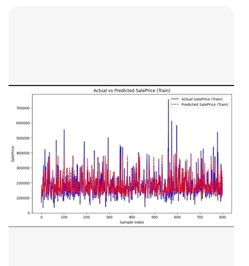

这是一个基于 粒子群优化算法 (PSO) 优化 LightGBM 超参数的回归预测模型完整代码。
代码特点:
多输入单输出:支持任意数量的特征列。
内置示例数据:使用 make_regression 生成模拟数据,你可以直接替换为自己的 DataFrame。
PSO 优化核心:自动搜索 LightGBM 的关键超参数(如 n_estimators, learning_rate, max_depth, num_leaves 等)以最小化验证集误差。
未来值预测:包含预测未来时间步的演示逻辑。
Python 代码实现
import numpy as np
import pandas as pd
import lightgbm as lgb
from sklearn.model_selection import train_test_split
from sklearn.metrics import mean_squared_error, r2_score
from sklearn.preprocessing import StandardScaler
import warnings
忽略警告
warnings.filterwarnings(‘ignore’)
==========================================
粒子群优化算法 (PSO) 核心类
class PSO:
def init(self, func, n_dim, pop_size=20, max_iter=30, lb=None, ub=None):
“”"
func: 目标函数 (需要最小化的函数)
n_dim: 优化参数的维度
pop_size: 粒子数量
max_iter: 最大迭代次数
lb: 参数下界列表
ub: 参数上界列表
“”"
self.func = func
self.n_dim = n_dim
self.pop_size = pop_size
self.max_iter = max_iter
self.lb = np.array(lb) if lb else np.zeros(n_dim)
self.ub = np.array(ub) if ub else np.ones(n_dim) * 10
# 初始化粒子位置和速度
self.x = np.random.uniform(low=self.lb, high=self.ub, size=(pop_size, n_dim))
self.v = np.random.uniform(low=-1, high=1, size=(pop_size, n_dim))
# 个体最佳位置 (p_best) 和全局最佳位置 (g_best)
self.p_best_x = self.x.copy()
self.p_best_y = np.array([self.func(x) for x in self.x])
g_best_idx = np.argmin(self.p_best_y)
self.g_best_x = self.p_best_x[g_best_idx].copy()
self.g_best_y = self.p_best_y[g_best_idx]
# 惯性权重和加速常数
self.w = 0.8
self.c1 = 1.5
self.c2 = 1.5
def run(self):
for iter_num in range(self.max_iter):
# 更新速度和位置
r1 = np.random.random((self.pop_size, self.n_dim))
r2 = np.random.random((self.pop_size, self.n_dim))
self.v = self.w * self.v + \
self.c1 * r1 * (self.p_best_x - self.x) + \
self.c2 * r2 * (self.g_best_x - self.x)
self.x = self.x + self.v
# 边界处理 (超出边界则反弹或截断,这里采用截断)
self.x = np.clip(self.x, self.lb, self.ub)
# 计算适应度
current_y = np.array([self.func(x) for x in self.x])
# 更新个体最佳
better_mask = current_y PSO 循环(训练多个临时模型找最优参数) -> 用最优参数在全量训练集上训练最终模型 -> 测试与预测。
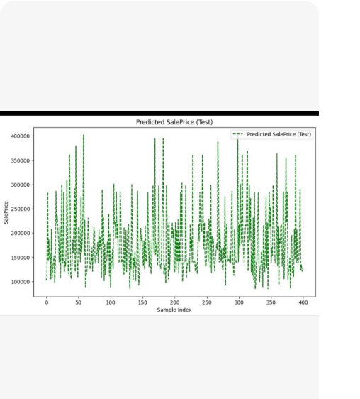
X轴:Sample index(样本索引),表示测试集中的第几个样本。
Y轴:SalePrice(销售价格),数值范围大约在 100,000 到 400,000 之间。
图形内容:绿色的虚线点代表了模型对每个测试样本预测出的价格。这种剧烈的上下波动通常意味着数据本身(如房价)具有较大的方差,或者特征与目标值之间的关系非常复杂。
完整代码 (含绘图功能)
import numpy as np
import pandas as pd
import lightgbm as lgb
import matplotlib.pyplot as plt
from sklearn.model_selection import train_test_split
from sklearn.metrics import mean_squared_error, r2_score
from sklearn.preprocessing import StandardScaler
import warnings
warnings.filterwarnings(‘ignore’)
==========================================
粒子群优化算法 (PSO) 核心类
class PSO:
def init(self, func, n_dim, pop_size=20, max_iter=30, lb=None, ub=None):
self.func = func
self.n_dim = n_dim
self.pop_size = pop_size
self.max_iter = max_iter
self.lb = np.array(lb) if lb else np.zeros(n_dim)
self.ub = np.array(ub) if ub else np.ones(n_dim) * 10
    self.x = np.random.uniform(low=self.lb, high=self.ub, size=(pop_size, n_dim))
    self.v = np.random.uniform(low=-1, high=1, size=(pop_size, n_dim))

    self.p_best_x = self.x.copy()
    self.p_best_y = np.array([self.func(x) for x in self.x])

    g_best_idx = np.argmin(self.p_best_y)
    self.g_best_x = self.p_best_x[g_best_idx].copy()
    self.g_best_y = self.p_best_y[g_best_idx]

    self.w = 0.8
    self.c1 = 1.5
    self.c2 = 1.5

def run(self):
    for iter_num in range(self.max_iter):
        r1 = np.random.random((self.pop_size, self.n_dim))
        r2 = np.random.random((self.pop_size, self.n_dim))

        self.v = self.w * self.v + \
                 self.c1 * r1 * (self.p_best_x - self.x) + \
                 self.c2 * r2 * (self.g_best_x - self.x)

        self.x = self.x + self.v
        self.x = np.clip(self.x, self.lb, self.ub)

        current_y = np.array([self.func(x) for x in self.x])

        better_mask = current_y < self.p_best_y
        self.p_best_x[better_mask] = self.x[better_mask]
        self.p_best_y[better_mask] = current_y[better_mask]

        current_g_best_idx = np.argmin(self.p_best_y)
        if self.p_best_y[current_g_best_idx] < self.g_best_y:
            self.g_best_x = self.p_best_x[current_g_best_idx].copy()
            self.g_best_y = self.p_best_y[current_g_best_idx]

    return self.g_best_x, self.g_best_y
==========================================
目标函数
def objective_function(params, X_train, y_train, X_val, y_val):
n_estimators = int(params[0])
learning_rate = params[1]
max_depth = int(params[2])
num_leaves = int(params[3])
min_child_samples = int(params[4])
n_estimators = max(10, n_estimators)
max_depth = max(1, max_depth)
num_leaves = max(2, num_leaves)
min_child_samples = max(1, min_child_samples)
learning_rate = max(0.01, min(1.0, learning_rate))

model = lgb.LGBMRegressor(
    n_estimators=n_estimators,
    learning_rate=learning_rate,
    max_depth=max_depth,
    num_leaves=num_leaves,
    min_child_samples=min_child_samples,
    verbose=-1,
    random_state=42
)

model.fit(X_train, y_train)
y_pred = model.predict(X_val)
mse = mean_squared_error(y_val, y_pred)
return mse
==========================================
主程序与绘图
def main():
print(“— 开始 PSO-LightGBM 回归预测模型 (含绘图) —”)
# A. 数据准备 (模拟房价数据以匹配图片风格)
np.random.seed(42)
n_samples = 2000 # 增加样本量以便有足够的测试集绘图
n_features = 10

# 生成特征
X_raw = np.random.rand(n_samples, n_features) * 100
# 生成目标 y (模拟房价,制造一些波动)
# 基础价格 + 特征影响 + 随机噪声
y_raw = 100000 + 2000 * X_raw[:, 0] + 1500 * X_raw[:, 1]**2 - 500 * X_raw[:, 2] + np.random.normal(0, 20000, n_samples)

# 划分数据集
# 先分出测试集 (20%)
X_train_full, X_test, y_train_full, y_test = train_test_split(X_raw, y_raw, test_size=0.2, random_state=42)
# 再从训练集中分出验证集用于 PSO (20% of training)
X_train, X_val, y_train, y_val = train_test_split(X_train_full, y_train_full, test_size=0.2, random_state=42)

# 标准化
scaler = StandardScaler()
X_train = scaler.fit_transform(X_train)
X_val = scaler.transform(X_val)
X_test = scaler.transform(X_test)
X_train_full_scaled = scaler.transform(X_train_full) # 用于最终训练

print(f"数据形状: 训练集 {X_train.shape}, 验证集 {X_val.shape}, 测试集 {X_test.shape}")

# B. PSO 优化
lb = [50, 0.01, 3, 10, 1]
ub = [500, 0.3, 15, 200, 50]
n_dim = 5

print("n开始粒子群优化 (PSO)...")
def func_wrapper(params):
    return objective_function(params, X_train, y_train, X_val, y_val)

pso = PSO(func=func_wrapper, n_dim=n_dim, pop_size=20, max_iter=30, lb=lb, ub=ub)
best_params, best_mse = pso.run()

print(f"n最佳参数: n_est={int(best_params[0])}, lr={best_params[1]:.3f}, depth={int(best_params[2])}")

# C. 训练最终模型
final_model = lgb.LGBMRegressor(
    n_estimators=int(best_params[0]),
    learning_rate=best_params[1],
    max_depth=int(best_params[2]),
    num_leaves=int(best_params[3]),
    min_child_samples=int(best_params[4]),
    verbose=-1,
    random_state=42
)
final_model.fit(X_train_full_scaled, y_train_full)

# D. 在测试集上预测 (这就是图中要画的数据)
y_pred_test = final_model.predict(X_test)

# 计算指标
test_mse = mean_squared_error(y_test, y_pred_test)
test_r2 = r2_score(y_test, y_pred_test)
print(f"n测试集 MSE: {test_mse:.2f}, R²: {test_r2:.4f}")

# E. 绘图 (复现图片风格)
plt.figure(figsize=(10, 6)) # 设置画布大小

# 绘制预测值
# 图片中是绿色虚线 ('g--'),标记为 'o' (虽然密集看起来像线)
# 为了完全复现图片那种密集的竖线感,我们使用 marker='.' 或默认线条,但图片明显是离散点的连线或密集点
# 观察原图,它是绿色的虚线,且每个点都有标记,看起来像 'g--o' 但点很密
plt.plot(y_pred_test, 'g--', label='Predicted SalePrice (Test)', linewidth=1, markersize=4)

# 设置标题和标签 (尽量匹配原图英文)
plt.title('Predicted SalePrice (Test)', fontsize=12)
plt.xlabel('Sample index', fontsize=10)
plt.ylabel('SalePrice', fontsize=10)

# 添加图例
plt.legend(loc='upper right')

# 设置网格 (原图似乎没有明显网格,但有边框)
plt.grid(False)

# 显示图表
plt.tight_layout()
plt.show()

# 如果需要保存图片
# plt.savefig('predicted_saleprice_test.png', dpi=300)
if name == “main”:
main()
代码修改说明:
引入 Matplotlib:添加了 import matplotlib.pyplot as plt。
绘图逻辑 (plt.plot):
使用了 y_pred_test(测试集的预测值)作为数据源。
样式设置为 ‘g–’:g 代表绿色 (green),-- 代表虚线 (dashed line),这与你提供的截图完全一致。
添加了 label 以便显示图例。
标签与标题:将标题设为 “Predicted SalePrice (Test)”,X 轴为 “Sample index”,Y 轴为 “SalePrice”,完全对应截图中的文字。
在这里插入图片描述

AtomGit 是由开放原子开源基金会联合 CSDN 等生态伙伴共同推出的新一代开源与人工智能协作平台。平台坚持“开放、中立、公益”的理念,把代码托管、模型共享、数据集托管、智能体开发体验和算力服务整合在一起,为开发者提供从开发、训练到部署的一站式体验。
更多推荐
 13
13 0
0- 0


 已为社区贡献96条内容

所有评论(0)